Fractional Fourier transforms and their optical implementation: I

(1)

Vol. 10, No. 9/September 1993/J. Opt. Soc. Am. A 1875

Fractional Fourier transforms and their optical

implementation:

I

David Mendlovic

Faculty of Engineering, Tel Aviv University, 69978 Tel Aviv Israel Haldun M. Ozaktas

Department of Electrical Engineering, Bilkent University, 06533 Bilkent, Ankara, Turkey Received November 30, 1992; accepted March 1, 1993

Fourier transforms of fractional order a are defined in a manner such that the common Fourier transform is a special case with order a = 1. An optical interpretation is provided in terms of quadratic graded index media and discussed from both wave and ray viewpoints. Several mathematical properties are derived.

1. MOTIVATION

It is often the case that an operation originally defined for integer orders can be generalized to fractional or even complex orders in a meaningful and useful way. A basic example is the power operation. The ath power of x, de-noted by Xa, might be defined as the number obtained by

multiplying unity a times with x. Thus X3= X X X X X. This definition makes sense only when a is an integer. However, it is an elementary fact that the definition of the power of a number can be meaningfully and consistently extended to real and complex values of a. Likewise, the original definition of the derivative of a function makes sense only for integral orders; that is, we can speak of the first or the second derivative and so on. However, it is possible to extend the definition of the derivative to non-integer orders by the use of an elementary property of Fourier transforms. Letting S[f

(x)]

denote the Fourier transform of the function f(x), defined as

KAfx)]= f(x)exp(-i27rf~x)dx, (1)

one has the property

(-i2irf )a9;[f(X)] _{= 9}₁

{da

]1

(2)

for integer a. Since the left-hand side of Eq. (2) is well defined for fractional values of a as well, it can be

consid-ered as the definition of the right-hand side of Eq. (2) for

real a. Bracewell showed how fractional derivatives can be used to characterize the discontinuities of certain func-tions.1 [A similar definition of fractional derivatives was

given long ago by Weyl (see Refs. 2 and 3). Fractional

integration is defined similarly.] Based on these two examples, one is led to ask from a mathematical viewpoint whether the definition of Fourier transforms can also be extended to fractional orders.

Fourier transforms (or their generalization, Laplace transforms) play a central role in the study of linear sys-tems.' They are also important in modern optics because

0740-3232/93/081875-07$06.00

the Fourier transform arises naturally in optical systems. This fact has been the central cause for the widespread use of information processing principles in optics and of optical systems for information processing. (In fact, one often encounters the term Fourier optics being used syn-onymously with optical information processing.)

In an optical system involving many lenses the axial locations of the images of the input object can be deter-mined by repeated application of familiar lens equations. Between these image planes it is possible to use the same equations to find the locations where the source would be imaged if no object were present in the system. The light distribution at these locations will have the form of the Fourier transform of the object,4so that these planes are called Fourier-transform planes. Thus, in a system in-volving many lenses, one can observe the object and its Fourier transform, the object's inverted image and its Fourier transform, the object's upright image and its Fourier transform, and so on. What we will call the first Fourier transform is the common Fourier transform. For the class of functions known as self-Fourier functions, the first Fourier transform is identical to the function it-self.5 The second Fourier transform is the Fourier trans-form of the first Fourier transtrans-form and is identical in form to f(-x, -y). The fourth Fourier transform is al-ways equal to the original function. From an optical viewpoint, one is led to inquire what is observed in such a system in the space between the images and the Fourier transforms and what is the effect of introducing spatial filters in these planes in addition to the conventional Fourier plane filter. Of course, the light distribution at any axial position can be calculated by the use of the Fresnel integral4; however, this fact is not very interesting unless it can be tied to other concepts and frameworks.

An example of a different kind of fractional operation from optics is related to the Talbot effect,6 in which self-images of an input object are observed at the two-dimensional planes z = Nzo for integer N (z is the axial coordinate and zo is a characteristic distance). By means of a self-transformation technique' it was shown that N could also take on certain rational values.

(D 1993 Optical Society of America

(2)

1876 J. Opt. Soc. Am. A/Vol. 10, No. 9/September 1993 In Ref. 8 the authors gave an example of a fractional Fourier transform without knowing so. In this reference a self-imaging configuration containing an odd number of identical systems is suggested. If it is noted that self-imaging is a Fourier transform with order a = 4, each of the identical systems could be considered as a fractional Fourier transformer with order a = 4/N, where N is an odd integer. However, the authors of Ref. 8 did not notice this point.

Based on the above motivations, one might be tempted to define the functional forms of the light distributions ob-served in these intermediary planes as fractional Fourier transforms. We will be arguing that such conventional Fourier-transforming configurations are not a good basis for defining fractional Fourier transforms because the dual actions of focusing and propagation are not uniformly interleaved in such systems. Rather, we will base our definitions on propagation in graded index (GRIN) media.9 Such media also exhibit imaging and Fourier-transforming properties and provide a natural environ-ment for defining fractional Fourier transforms.

In Section 2 we will introduce the notation and the basic postulates that we will require our definition to satisfy. Afterward we will discuss why GRIN media provide a natural environment for the definition of fractional Fourier transforms. Then propagation in GRIN media will be reviewed and the fractional Fourier transform defined mathematically in conjunction with its optical interpretation in GRIN media. After discussing some of the elementary properties of the fractional Fourier trans-form, we will examine our definition using ray optics in phase space and show that it indeed has some attractive properties.

In the sequel to this paper0 we will provide illustrative examples of fractional Fourier transforms and discuss some extensions and generalizations. We will discuss how fractional Fourier transforms can be obtained with bulk

systems. Also, we will show how to generalize the spatial

filtering process based on fractional Fourier transforms as well as on some computer simulations.

The fractional Fourier transform has previously been defined by mathematicians in a purely abstract way as a novel method of solving the Schr8dinger equation under various conditions."'2 _{Given the analogy between} Maxwell's equations in GRIN media and the Schrodinger equation for the harmonic oscillator, this dual definition is not surprising. However, the authors of Refs. 11 and 12 did not mention the possibility of an optical interpretation. Note that these mathematicians did not suggest physical applications for their fractional Fourier-transform defini-tion. Owing to the major significance of the Fourier transform in optics, we assume that this new operator, motivated by the GRIN media, will be more useful in the optics community. In Ref. 10 an application for optical signal processing is suggested. Another application for this operator could be to solve the harmonic-oscillator problem.

2. NOTATION AND BASIC POSTULATES The ath Fourier transform of a function f(x, y) will be

de-noted as 9a[f(x, y)] or simply as S;af when there is no

con-fusion. We require that our definition satisfy two basic

postulates. First, l;

'f

should be the usual first Fourier transform (the Fourier property), defined as

(9; 1f)(', y') =

f

f(x, y)exp[ T( 2 YY)ldxdy

(3) where s, x, x', y, and y' all have the dimensions of length. In a conventional 2f optical Fourier-transforming configu-ration'3 (x, y) would denote the coordinates of the input plane, (x', y') would denote the coordinates of the Fourier plane, and s2 = Af (A is the wavelength of light and f is the

focal length of the lens). The parentheses on the left-hand side of Eq. (3) emphasize that the variables (x', y') belong to the function ('f) and not f

Our second postulate requires that

sa[obf] = sasbf = bsaf = ;a+bf;

(4)

that is, repeated applications of the fractional Fourier transform operator Sa should be additive (the semigroup

property).

3. GRADED INDEX MEDIA AS A BASIS FOR DEFINING FRACTIONAL FOURIER

TRANSFORMS

GRIN media will play a central role in our definition of fractional Fourier transforms. To motivate their use, we first discuss them as the limiting case of a cascade of a larger and larger number of weaker and weaker focusing

systems.

Let us begin by recalling that the common optical Fourier-transform operation has two ingredients, free-space propagation and focusing by a positive lens. We can speak of these operations as being duals or Fourier conju-gates of each other.4"4 Indeed, as discussed in Ref. 4, the effects of propagation and focusing on an incident light distribution can be described by convolution and multipli-cation, respectively, by functions of the same form,

exp[-iir(x2 + y2)/C], (5) where C = AAz for propagation over a distance Az and

C = -Af for focusing by a lens of focal length f

In a conventional 2f Fourier-transforming configuration the act of focusing is fully concentrated at the lens and segregated from the act of propagation. We can define 9"1 2f by distributing the focusing through the propagation

as shown in Fig. 1. The distance 1 and the focal power f1/2

are chosen so that two such systems in cascade yield the first Fourier transform of the input. One can find that, for any arbitrary length f[, the two free parameters of this configuration are

f1/2 = f,/sin(,r/4), 1 = f' tan(qr/8). (6)

Consistent with our two postulates, we can now extend this argument to define 0;l1Q[.] for integer Q as that opera-tion which, when applied Q times, gives the first (conven-tional) Fourier transform of f An optical system that performs this operation may be realized by the insertion of a lens of appropriate focal length midway between the D. Mendlovic and H. M. Ozaktas

(3)

input output*

I |

Fig. 1. Optical setup for defining the 9;1I2 operator.

appropriately spaced input and output planes, as in Fig. 1.

Then f',Q and I become

AIQ = - /Q 1 = Ai tan(4) (7)

sin(iT/2Q)

k4Q!

respectively.

It is now possible to define Fourier transforms of rational order i;'IQf by repeated application (P times) of the opera-tor ?;l/Q. The definition can be generalized to real orders by a limiting process.

To repeat, in a conventional 2f system the focusing action is concentrated at the lens location. The same op-eration can also be performed by Q fractional Fourier-transform stages in cascade, each performing 9i;'Q[-]. Note that the larger Q is, the more evenly distributed the

focusing action becomes and the less segregated it be-comes from the propagation action. In the limit Q -m

-focusing and propagation will be infinitesimally and uni-formly interspersed between each other. Of course, bulk systems with even moderately large Q would be quite im-practical. Fortunately, systems satisfying the same prop-erty can be realized as quadratic GRIN media. Such media can be regarded as consisting of infinitesimal layers in which focusing and propagation take place simul-taneously. This property is apparent on examination of the refractive index distribution of such media,'5

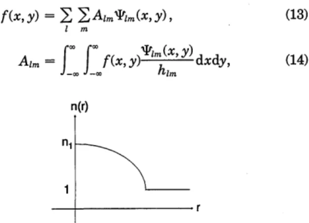
n2(r) = nl[1 - (n2/nl)r2], (8) where r2 = x2 + y2 is the radial distance from the optical axis and nj, n2 are the GRIN medium parameters.

Figure 2 shows a typical refractive index profile of such a

quadratic GRIN medium. As is commonly done, we

as-sume that the field distributions of interest are confined to a neighborhood of the optical axis such that the value of n(r) dictated by the above equation is -1. By solving the ray equation, one can show" that a parallel bundle of rays will be focused a distance L = (/2)(n,/n 2?2 from the

input plane. In Section 6 we show that if a function f(x, y) is presented at the input plane z = 0, then at the plane

z = L we observe 9;f as given by Eq. (3). In other words,

the focusing property of GRIN media is confirmed from a

wave optics viewpoint as well. Now, since the system is

fully uniform in the axial direction, 9;f can be physically defined as the functional form of the scalar light distribu-tion at z = aL. Note that this definidistribu-tion would not be relevant in a bulk system, since the focusing and the propagation are not uniformly interleaved in that case.

Above we have motivated and defined the fractional Fourier transform in physical terms. However, it is im-portant to note that fractional Fourier transforms can be defined purely mathematically (as in Refs. 11 and 12) and GRIN media introduced afterward as a physical interpre-tation. The mathematical definition will be presented in the. following sections, along with its connection to

propa-gation in GRIN media. We will return to discuss bulk systems in greater detail in the sequel to this paper.'0

Although we cannot exclude the possibility of other defi-nitions consistent with our two postulates, our particular definition is seen to be a natural and meaningful one, es-pecially in an optical context.

4. REVIEW OF PROPAGATION IN GRADED INDEX MEDIA

The self-modes of circular quadratic GRIN media are the members of the Hermite-Gaussian (HG) function set. All the members of this self-mode set are mutually orthogonal. This function set is also an infinite and orthogonal solu-tion set of the Schr6dinger equasolu-tion for the harmonic os-cillator.5"6 As such, it is also complete.

The HG functions have the form

'Pm(XY) = H( x)Hm(

c2Yexp(

- 2) ₍₉₎

where H, and Hm are Hermite polynomials of orders 1 and m, respectively,

w= (2/k)112(nl/n2)14, (10)

with k = 2rn,/A, and A is the wavelength. Each HG mode propagates through the GRIN medium with a different propagation constant'5

f8im =

k[1

-

2(n)1/2

+ M + 1)]

(11)

k(

)n2

1/2+M+1).

As a result of Eq. (9) and relation (11) the field distribu-tion of a specific mode (1, m) that propagates through the medium can be written as

Elm(X, yZ) = Wlm(x, y)exp(i6,mz) - (12)

5. FORMAL DEFINITION OF FRACTIONAL FOURIER TRANSFORMS

Because of the orthogonality and the completeness of the HG function set, every two-dimensional function f(x, y) can be expressed as f (x, y) = 2 Aim'Pim (x, y), I m Alm =

£

f(x, Y) m(X, Y dxdy, foo _o fhim (13) (14) n(r) ni Fig. 2. Typical medium.

refractive index profile of a quadratic GRIN

D. Mendlovic and H. M. Ozaktas

(4)

1878 J. Opt. Soc. Am. A/Vol. 10, No. 9/September 1993 where

him = 21+ml! m! rno2/2. (15)

Now the fractional Fourier transform of f(x, y) of order a can be defined as

9;a[f(x,y)] =

I 2AimWPm(xy)exp(i,6jmaL).

I m

(16) As discussed in Section 2, we require that our fractional Fourier-transform definition satisfy two postulates, the Fourier [Eq. (3)] and semigroup [Eq. (4)] properties. The second can be proved directly from Eq. (16). Let us apply the operator 9b to the right-hand side of Eq. (16):

9b[9af] = 2 A;mb AWmm(x, y)exp(iI3zniaL)

= > AimWlm(xsy)exp[iIl~im(a + b)L] = 21a+bf.

I m

(17)

n = 0 and n = 1; then we assume that it holds for n - 1

and n and show that this assumption implies that the hy-pothesis holds for n + 1. Our hyhy-pothesis is that

(23) Let us check it for n = 0:

9'[PO(x')]

=

f

exp(-

- 2 x)dx'.

With the well-known mathematical integral9

7

exp(-p 2x2 + qx)dx =exp p

P

(24)

(25) we see that Eq. (24) follows exactly the induction assump-tion (23). Since the recursive definiassump-tion [Eq. (21)] depends on two previous orders, we must demonstrate that our hy-pothesis also holds for n = 1. This demonstration can be performed in a similar way with the use of the integral9 The more complicated proof of the Fourier property

is given in Section 6. In this proof we mathematically confirm that the a = 1st Fourier transform, as defined above, is indeed equivalent to the standard definition given in Eq. (3), provided that we choose the scale factor s

[see Eq. (3)], where

s =

7. (18)

Readers who are willing to accept the above results on faith may skip to Section 8.

6. PROOF OF THE SEMIGROUP PROPERTY

In this section we prove Eq. (3) for the fractional Fourier-transform definition of Section 5. For the sake of notational compactness, we present the proof for one-dimensional functions. The extension to two dimensions is straightforward.

The strategy of the following proof is to calculate the right-hand side of Eq. (3) for each HG function and to compare the result with the left-hand side with the use of

definition (16).

The Hermite polynomials could be calculated with7

Hn(x) = (-1)nexp(x2) d exp(-x2), (19)

which leads to the following lower-order polynomials:

Ho(x) = 1, Hl(x) = 2x, H2(x) = 4X2- 2. (20)

A recursive definition of the Hermite polynomials is'8

H.+,(x) = 2xHn(x) -2nHn-(x) (21)

fx

exp(-px

2

+ 2qx)dx =

(9

-)

exp(

-). (26)

Now we assume that our hypothesis holds for n - 1 and

n and show that this assumption implies that the

hypothe-sis holds for n + 1. For this purpose we use the recursive definitions (21) and (22). Finally, we obtain

(27)

exactly as our hypothesis predicts.

For the sake of comparison with Eq. (16), we can rewrite Eq. (23) as

= Tn(x)\-/roj exp(-inir/2). (28) Comparing Eqs. (16) and (28), we observe that

L=

(2/4)(n/n2)1'2, (29) which is exactly the focal length that is obtained with ray

optics.'"

7. BASIC PROPERTIES

In this section some of the mathematical properties of the fractional Fourier-transform operator are investigated.

Linearity

Let us denote two original functions by the lowercase let-ters f(x) and g(x). If

9;f(x)

and 9;ag(x) are the respective fractional Fourier transforms, then

a [Clf(x) + C2g(x)] = C19f(X) + C29g(x), (30)

or'9

dHn(x) = 2nHn-,(x).

dx

The following proof uses the induction technique over n. That is, we first demonstrate that our hypothesis holds for

where cl and c2are complex constants.

The proof of this property is based on defining the HG components of f(x) and g(x), namely, Af and A9, respec-(22) tively, such that

n

f(x)

= Aft(x), g(X) =Ag

/ - n n gx-nn .

n n (31)

gl[,pn(X,) = N/-,IT (0,pn (X) (_ i)n.

(5)

Vol. 10, No. 9/September 1993/J. Opt. Soc. Am. A 1879 Because of the linearity of the integral operation, one can

notice that the HG components of Clf + ₂g are cjAf +

c2Ag, and thus

Clf(X) + C2g(X) =

I(cAf

+ 2An)Pn(x), n

(32)

which leads directly to Eq. (30). Continuity

For two fractional Fourier-transform operations with orders a, and a2, we can write

91cja1+c2a2f(x) = ;cja19;c2a2f(x) = ;C2a29;claf(X).

(33)

The proof makes use of Eq. (16):

9;cja1+c2a2f(x) =

2AfT,(x)exp[-iP3L(cjaj

+ c2a2)] n =

EAfn

exp(-if39Lcjaj)exp(-i,38Lc 2a2) n = icla1[ Af

exp(-iGnLc

2

a

2

)Tn(x)1

= 9;cla19;c2a 2f(x)

(34)

A similar procedure can be followed for proving the second equality in Eq. (33).

Self-Imaging

An interesting special case of Eq. (33) arises when c2a2 =

4. Then

9jcjaj+ 4f(X) = 9cjlaj9; 4f(X) = 9;cjaf(x) (35)

That is, the above condition leads to self-imaging of the transformed plane. Note that for self-Fourier functions (see Ref. 7) self-imaging is also obtained for c2a2 = 1.

Partial Convolution/Correlation

A possible definition for the convolution operation of f(x) and g(x) is

CONV(f,g) = 9;-1[9;lf(x) x VI~'g(x)]. (36)

Let us denote this operation as the a = 1st convolution. Based on the fractional Fourier-transform definition, a convolution with the fractional order a is defined as

CONV (g) = 9;-a[9;af(x) X 9;ag(X)]. The fractional correlation is similarly defined as

CORRa[f(x),g(x)] = CONVa[f(x), g*(-x)].

(37)

Differentiation Rule 9ga[Drf(y)](x)

= [-ix sin(2qra) + cos(21ra)D] 9;a[f(y)](x). (40)

Mixed Product Rule

9;a[(yD)rf(y)](x) = {-[sin(2ra) + ix2 cos(2ara)]sin(21ra)

+ x cos(2ira)D - i sin(2ra)

X cos(2,7ra)D 2}mS;a[f(y)](x). (41)

Shift Rule

9ja5b[f(y)](x) = exp(-ib sin{2ira[x + 0.5b cos(2a)]}) x 9;a{f(y)}[x + b cos(2ira)],

where jb denotes the shift operator:

ETb[f](x) = f(x + b).

(42)

(43)

One can notice from this rule that the intensity of the transformed shifted function is always the same; in other words, the intensity is shift invariant.

Exponential Rule

ga{exp(iby)f(y)}(x) = exp(ib cos{2lra[x + 0.5b sin(2ira)]})

x 9;a{f(y)}[x + b sin(2ira)]. (44)

8. RAY-OPTICS INTERPRETATION

We will now examine the behavior of optical fractional Fourier transforms from a ray-optics viewpoint. In doing so, we will make use of a phase-space representation, which is also closely related to the well-known matrix for-mulation of ray optics.18

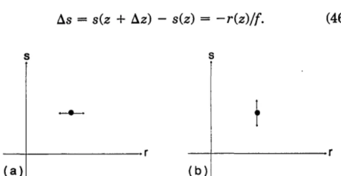
Let a particular paraxial ray be characterized by its ra-dial distance r and slope s, both with respect to the optical axis at a particular axial position z. Then the effect of passing through any optical system on this ray can be described as a movement in (r, s) space. For instance, free-space propagation over a length Az corresponds to a horizontal displacement Ar given by [Fig. 3(a)]

Ar

= r(z +

Az)

- r(z) = s(z)Az. (45)

On the other hand, focusing by a lens of focal length f corresponds to a vertical displacement by [Fig. 3(b)]

(38)

Additional Properties

In their papers Namias" and McBride and Kerr2 obtained some additional properties of the fractional Fourier-transform operation. These results are given below without their mathematical proofs:

Multiplication Rule

g1a[ymf(y)](x) = [x cos(2ira) - i sin(27ra)D]rmIa[f(y)](x),

(39)

where D denotes the differential operator d/dx.

As = s(z + Az) - s(z) = -r(z)/f.

s

(46)

t

(a)I (b)I

Fig. 3. Effect of (a) propagation and (b) focusing by a lens on a

given ray in (r, s) space.

r .r~~~~~~~~~~~~~~

(6)

1880 J. Opt. Soc. Am. A/Vol. 10, No. 9/September 1993

(a) (b)

s

(d)I (c)I

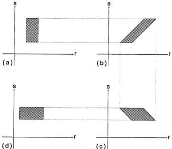
Fig. 4. Phase-space representation of the original bundle of rays (a), after free-space propagation through a distance f (b), after

passage through a lens of focal length f (c), and after another free-space propagation through a distance f (d).

Let us now consider a bundle of rays with a uniform spread of r and s [represented by the crosshatched rectan-gular region in Fig. 4(a)] and consider how this ray bundle is transformed as it passes through a conventional 2f Fourier-transforming configuration (Fig. 4). The overall effect of the 2f system is to rotate the rectangular region by 900, although the intermediate steps result in shearing of the rectangular region.

We now examine the effect of fractional Fourier trans-forming in GRIN media on the rectangular region in Fig. 4(a). It is known that r and s obey the following equations in such media":

r(z + Az) = r(z)cos(7rAz/2L) - s(z)sin(7rAz/2L),

s(z + Az) = r(z)sin(irAz/2L) + s(z)cos(rAz/2L), (47)

from which we can conclude that the region representing any given bundle of rays in phase space is uniformly

ro-tated as z is increased. An increment of Az = L, a full

Fourier-transform distance, corresponds to a rotation by 90°. This uniform behavior is to be contrasted with that of the bulk 2f Fourier transformer, in which the focusing is concentrated at the lens instead of being uniformly dis-tributed throughout the system. For this reason it is not attractive to define fractional Fourier transforms based on conventional Fourier-transforming systems.

9. CONCLUSION

We have defined the fractional Fourier-transform operator

9;a such that the common Fourier-transform operator is a

special case with a = 1. Our optically motivated defini-tion was seen to be identical to a purely mathematical derivation found in the mathematics literature. We dis-cussed several properties of this transform, in particular showing that they can be realized with quadratic graded index (GRIN) media. Although the definition of the frac-tional Fourier transform is not unique, our definition is useful from the physical optical point of view. The two

postulates on which the definition is based are well matched to a very useful optical device-the GRIN medium.

Fractional Fourier transforms can form the basis of generalized spatial filtering operations, extending the range of operations possible with optical information pro-cessing systems. Conventional Fourier plane filtering systems'3 are based on a spatial filter introduced at the Fourier plane, which limits the achievable operations to space-invariant ones. By introducing several filters at different fractional Fourier planes, one can implement a wider class of operations.

It is important to note that, although they provide a con-text for defining fractional Fourier transforms in a satis-fying manner, GRIN media may not be good candidates for practical implementation, especially because they can-not have large space-bandwidth products. For practical purposes, it is possible to simulate GRIN media by the use of bulk lenses such that the same light distribution will be observed at the planes in which filtering will take place.'

Several of the issues mentioned above will be taken up in the sequel to this paper.'0 In addition, we will provide illustrative examples of fractional Fourier transforms and introduce some extensions and generalizations.

ACKNOWLEDGMENTS

Some of the ideas in this paper were developed during in-tensive study sessions organized by Adolf W Lohmann at the Applied Optics Group of the University of Erlangen-Niirnberg during the summer of 1992. The authors ac-knowledge the useful suggestions of Klaus Leeb of the Informatik Department of the University of Erlangen.

REFERENCES

1. R. Bracewell, The Fourier Transform and Its Applications,

2nd ed. (McGraw-Hill, New York, 1986).

2. A. Zygmund, Trigonometric Series, 1 (Cambridge U. Press,

Cambridge, 1979).

3. P. I. Lizorkin, "Fractional integration and differentiation," in Encyclopedia of Mathematics (Kluwer, Dordrecht, The

Netherlands), Vol. 4.

4. A. Vander Lugt, Optical Signal Processing (Wiley, New York, 1992).

5. A. Lohmann and D. Mendlovic, "Image formation and self-Fourier object," submitted to Appl. Opt.

6. K. Patorski, "The self-imaging phenomenon and its applica-tions," in Progress in Optics, E. Wolf, ed. (North-Holland,

Amsterdam, 1989), Vol. 28, p. 3-110.

7. A. Lohmann and D. Mendlovic, "Self-Fourier objects and

other self-transform objects," J. Opt. Soc. Am. A 9, 2009-2012 (1992).

8. A. Lohmann and D. Mendlovic, "Optical self-transform with odd order," Opt. Commun. 93, 25-26 (1992).

9. H. Ozaktas and D. Mendlovic, "Fourier transforms of frac-tional order and their optical interpretation," Opt. Commun. (to be published).

10. H. Ozaktas and D. Mendlovic, "Fractional Fourier transforms and their optical implementation: II," J. Opt. Soc. Am. A

(to be published).

11. V. Namias, "The fractional Fourier transform and its applica-tion in quantum mechanics," J. Inst. Math. Its Appl. 25,

241-265 (1980).

12. A. C. McBride and F. H. Kerr, "On Namias's fractional Fourier transforms," IMA J. Appl. Math. 39, 159-175 (1987). 13. J. Goodman, Introduction to Fourier Optics (McGraw-Hill,

New York, 1968).

"I'"" I I...

.1 ...I...I... .I... ...I... ... ... ... I.. ... ... ...-.1 .... ...I ... 'a I

I...I...

.Nqm& ...

(7)

14. A. Lohmann, "Ein neues Dualitatsprinzip in der Optik," Optik (Stuttgart) 11, 478-488 (1954). An English version appeared in Optik (Stuttgart) 89, 93-97 (1992).

15. A. Yariv, Optical Electronics, 3rd ed. (Holt Reinhart, New

York, 1985).

16. A. Yariv, Quantum Electronics (Wiley, London, 1975).

17. A. Erdelyi, Tables of Integral Transforms (McGraw-Hill,

New York, 1954), Vol. 1, p. 369.

18. B. E. A. Saleh and M. C. Teich, Fundamental of Photonics (Wiley, New York, 1991).

19. M. Abramovitz and I. A. Stegun, Handbook of Mathematical Functions (Dover, New York, 1970).