1 November 1997
OPTICS COMMUNICATIONS
ELSEVIER Optics Communications 143 (1997) 75-86
Full length article
Relationships among ray optical, Gaussian beam, and fractional
Fourier transform descriptions of first-order optical systems
Haldun M. Ozaktas, M. Fatih Erden
Depurtment of Electricnl Engineering. Bilkmt University, TR-06533 Bilkent, Ankara, Turkey Received 15 January 1997; accepted 3 June 1997
Abstract
Although wave optics is the standard method of analyzing systems composed of a sequence of lenses separated by arbitrary distances, it is often easier and more intuitive to ascertain the function and properties of such systems by tracing a few rays through them. Determining the location, magnification or scale factor, and field curvature associated with images and Fourier transforms by tracing only two rays is a common skill. In this paper we show how the transform order, scale factor, and field curvature can be determined in a similar manner for the fractional Fourier transform. Our purpose is to develop the understanding and skill necessary to recognize fractional Fourier transforms and their parameters by visually examining ray traces. We also determine the differential equations governing the propagation of the order, scale, and curvature, and show how these parameters are related to the parameters of a Gaussian beam. 0 1997 Published by Elsevier Science B.V.
Keywords: Fourier optics; Optical information processing; Fractional Fourier transforms
1. Introduction
In this paper we consider centered optical systems composed of an arbitrary number of lenses separated by arbitrary distances (Fig. 4a), under the standard approximations of Fourier optics [l]. In such a system one can determine the output amplitude distribution of light in terms of the input amplitude distribution by employing wave optical methods. However. upon first inspection, we generally tend to ascertain the function and properties of such a system by tracing - on paper or in our imagination - a few rays or geometrical wavefronts through the system. For historical, psychological, and pedagogical reasons, ray optical methods play an important role in our understanding of the first-order properties of optical systems. A recent example of the usefulness of ray optics for the analysis of coherent imaging systems has been given by Rhodes [2]. Optical systems involving an arbitrary sequence of thin lenses separated by arbitrary sections of free space (under the Fresnel approximation) belon, u to the class of quadratic-phase svsrems ‘. (The class of Fourier optical systems (more precisely called first-order optical systems [3]) consist of arbitrary thin filters sandwiched between arbitrary quadratic-phase systems.) Members of the class of quadratic-phase systems 13-71 are characterized by linear transformations of the form
p,,,(x) =
Ix
h(x,x’)P,~( x’)
dx’.-77
h( x.x’) = Kexp[ in-( (Y-r2 - 2p.r.r’ + y-r”)]. (1)
where K is a complex constant, and (Y. p, and y are real constants.
’ Quadratic graded-index media also belong to this class and our results are easily extended to systems containing arbitrary sections of such media.
0030-4018/97/$17.00 0 1997 Published by Elsevier Science B.V. All rights reserved. PII SOO30-4018(97)00305-2
76 H.M. Ozaktas, M.F. Erden / Optics Communications 143 (1997) 75-86
The kernels associated with a thin lens with focal length f, and free-space propagation over a distance d are given respectively by [l]
hlens( x,x’) = Klens 6(x - n’) exp( -
inx’/hf)
,
&ad n 1 n’ > = &pace exp[ ir( x - x’)*/Ad]
A is the wavelength of light in free space. One-dimensional notation is employed for simplicity. These kernels are special cases of the kernel given in Eq. (1). It is possible to prove that any arbitrary concatenation of kernels of these forms will result in a kernel of the form given in Eq. (1) [4].
Apart from the constant factor K which has no effect on the resulting spatial distribution, a member of the class of
quadratic-phase systems is completely specified by the three parameters (Y, p. and y (Eq. (1)). Alternatively, such a system can also be completely specified by the transformation matrix [3-71
Y/P
l/P
-P+v/P
ff/P
1’
(4)
with AD - BC = 1. If several systems each characterized by such a matrix are cascaded, the matrix characterizing the overall system can be found by multiplying the matrices of the several systems [3,5,6]. The matrix defined above also corresponds to the well known ray matrix employed in ray optical analysis. At a certain plane perpendicular to the optical axis, a ray can be characterized by its distance from the optical axis x and its paraxial angle of inclination 0. We will define the ray vector as [x ~1~ where p = 0/h. Then, the ray vector at the output is related to the ray vector at the input by [l]
So as to provide a framework for discussing fractional Fourier transforming systems, we will first review two important special cases of the general class of systems under consideration, namely imaging and Fourier transforming systems. We will also allow for the case where the image or the Fourier transformation is obtained up to a residual quadratic-phase term. We will then consider the fractional Fourier transformation which includes both imaging and the common Fourier transformation as special cases. We will show that any quadratic-phase system can be interpreted as a fractional Fourier transform, up to a quadratic-phase term at the output.
Everyone well versed in Fourier optics can easily determine the image and Fourier transform planes in a system by sketching a few (usually two) rays. After reviewing these techniques, we will extend them to the fractional Fourier transform, showing how the order and other parameters of a fractional Fourier transform can be determined by sketching a few rays.
Everything discussed in this paper can be ascertained without the use of any ray optical concepts. However, given the experience and intuition invested in these concepts, it is easier to visually grasp the nature of an optical system by tracing a few rays, rather than by evaluating Gaussian integrals obtained by concatenating the kernels of subcomponents. Those who have studied elementary Fourier optics are already comfortable in their understanding of imaging and Fourier transforming systems in terms of ray optics. Our purpose is to extend this understanding and intuition, as much as possible 2, to the fractional Fourier transform. Indeed, many colleagues and students have complained that they are unable to visualize or intuitively grasp the formation of the fractional Fourier transform in the same way as they can visualize imaging or Fourier transforming operations.
Although ray optics is a special case of wave optics, it is often possible to extract a significant amount of information regarding a system by ray optical analysis alone. In fact, under the standard approximations of Fourier optics, the common class of systems we are analyzing can be described completely by ray analysis. (This does not mean that the field amplitudes around a caustic can be determined by ray optical analysis alone. It rather means that the overall behavior of the system can be fully characterized by ray optical parameters.) More precisely, examination of the behavior of a few rays will allow us to determine the matrix defined in Eq. (4), which will allow us to determine the parameters (Y, /3, y, which completely characterize the kernel defined in Eq. (l), which completely determines the transformation of the wave fields.
‘There is an intrinsic obstacle arising from the fact that the fractional Fourier transform is a more general and complicated transformation, so that we cannot expect its visualization and grasp to be as easy as its special cases.
H.M. Omktas, M. F. Erden / Optics Communications 143 (1997) 75-86 II
2. Imaging and Fourier transformation
We first discuss the historically prior case of imaging. The most general transform kernel, allowing for the possibility of a residual quadratic-phase term may be expressed as
/I( x,x’) = Kexp( irrx’/AR) 6( x - Mx’). (6)
This kernel maps a function p(x) to Kexp(i~x’/hR)IMI-‘p(x/M). M is referred to as the magnification and R is the radius of the spherical surface on which the perfect image is observed. When R = ~0, the quadratic-phase term disappears and the perfect image is observed on a planar surface. The above kernel is a special case of Eq. (1) with cr,p,y + 00 such that y/j3 = M, cy - j3 ‘/ y = l/AR. The matrix associated with the imaging kernel is given by
0
1
l/M
Now, interpreting T as a ray matrix, the following well recognized conditions may be deduced:
If and only if a given quadratic-phase system is an imaging system, a ray emanating from the axial point at the input plane (xi, = 0) is mapped onto the axial point at the output plane (x,,~ = 0) (Fig. la).
If a ray parallel to the optical axis at the input plane (ei, = 0) is also parallel to the optical axis at the output plane ( f?,,,, = 0), the imaging is perfect with no residual phase curvature ( R = M), and the magnification M is given by the ratio of the distance of the output ray to the optical axis, to the distance of the input ray to the optical axis: M = xOJxin (Fig. la).
If a ray parallel to the optical axis at the input plane is not parallel to the optical axis at the output plane, the magnification is found in the same way as in perfect imaging, and the radius of curvature of the residual quadratic-phase factor is simply that defined by the slope of the ray (R = x~,,/~,,,> (Fig. lb).
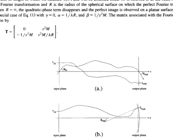
We now turn our attention to Fourier transformation. The most general transform kernel allowing for the possibility of a residual quadratic-phase term may be expressed as
h( x,x’) = K exp( in-x*/AR) exp( -i27rxx’/s2M). (8)
This kernel maps a function p(x) into Kexp(iPx2/AR)P(x/s2~), where P( ) is the Fourier transform of p( ). Here s is the unit of length in which we measure x,x’, and will be assumed fixed. M is referred to as the scale factor associated with the Fourier transformation and R is the radius of the spherical surface on which the perfect Fourier transform is observed. When R = ~13, the quadratic-phase term disappears and the perfect image is observed on a planar surface. The above kernel is a special case of Eq. (1) with y = 0, (Y = l/AR, and p = 1 /s2M. The matrix associated with the Fourier transform kernel is given by
s2M
1
- l/s=M s2M/AR
.
input plane
(a.> output plane
(9)
I
input plane
@.I
78 H.M. Ozaktas. M.F. Erden / Optics Communications 143 (1997) 75-86
input plane
(a.)
Input plane
(b.1
Fig. 2. Fourier transforming.
i’
output plane
Now, interpreting T as a ray matrix, the following well recognized conditions may be deduced:
If and only if a given quadratic-phase system is a Fourier transforming system, a ray parallel to the optical axis at the input plane (C&, = 0) will pass from the axial point at the output plane (x,,~ = 0) (Fig. 2a).
If a ray emanating from the axial point at the input plane (n,, = 0) emerges parallel to the optical axis at the output plane (e,,, = 01, the Fourier transformation is perfect with no residual phase curvature (R = m>, and the scale factor M is given by the ratio of the distance of the output ray to the optical axis, to the angle of the input ray: M = ~,,~h/f3,,s* (Fig. 2a). If a ray emanating from the axial point at the input plane does not emerge parallel to the optical axis at the output plane, the scale factor is found in the same way as in perfect Fourier transformation, and the radius of curvature of the residual quadratic-phase factor is simply that defined by the slope of the ray (R = x,,,//3,,,) (Fig. 2b).
Fractional Fourier transformation
Finally we can discuss the fractional Fourier transform within the same framework. The fractional Fourier transform [4,8-11) is also a subclass of the class of quadratic-phase systems. The transform kernel allowing for the possibility of a residual quadratic-phase term may be expressed as a
h( x,x’) = K exp(
where C$ = arr/2. The common Fourier transform is obtained when we set a = 1 and the common inverse Fourier transform is obtained when a = - 1. Ordinary imaging is obtained when a = 0 or a = f 2. This kernel maps a function p( x/s) into K’exp(i~x*/AR)p,(x/sM), where p,( 1 is the uth order fractional Fourier transform of p( ), and K’ is a
T= Mcos f$ s2Msin+
- sin4/s*M + Mcos +/A R cos 4/M + s2Msin +/A R I . (11)
A large number of papers deal with the fractional Fourier transform in an optical context. For instance, see Refs. [4,7,12-291 and references therein.
H.M. Ozaktas. M.F. Erden/Optics Communications 143 (1997) 75-86
input plane
(a.>
(W
/
input plane output plane
Fig. 3. Fractional Fourier transforming: (a) x,, = 0; (b) 8,” = 0.
For a given quadratic-phase system to be an imaging or Fourier transforming system, certain conditions had to be satisfied. However, we will see below that any quadratic-phase system can always be interpreted as a fractional Fourier transforming system, and that its parameters can be obtained by sketching only two rays and making three measurements. (This procedure can also be made the basis for the experimental characterization of the parameters of a given system.) Thus the fractional Fourier transform is general enough to describe all systems composed of an arbitrary number of lenses separated by arbitrary distances, whereas imaging and Fourier transforming systems are only special cases.
We first consider any ray parallel to the optical axis at the input plane (0,” = 0) (Fig. 3b). Our first measurement p is given by the ratio of the distance of the output ray to the optical axis, to the distance of the input ray to the optical axis ( p = x,,~/x,,). Our second measurement is the radius of curvature p defined by the output ray ( p = x,,,/@,~~). We then consider any ray emanating from the axial point at the input plane (xi, = 0) (Fig. 3a) and take the radius of curvature @ defined by the angle q,, it makes at the output plane as our third measurement. A fourth measurement defined by u = X,,t A/s%,,, while redundant, will simplify calculations. (By employing the unit determinant condition AD - BC = 1, CT can be shown to be related to the other measurements p. p, Q by the equation S%F( Q- ’ - p- ’ ) = h.) Now. Eqs. (5) and (11) allow us to write the equations
McosCp = /.l. (12) Msin+= cr. (13) tan4 1 1 --+hR=-. s’M 2 AP (14) cot4 1 1 -+t=-. S2M2 he (15)
Again, any one of these equations, for instance the one involving (T, can be derived from the other three using the unit determinant condition and is thus redundant. By using the first three equations and since M > 0 we obtain the unique solution tan+= “, P M=y’p’+o’, 1 A ff/I* 1 -= --+--_ R .s2 pz+(Tz p
The quadrant of C$ is determined uniquely by the signs of k and cr. The dependence on s’crp( eP’ -pm’) = A, if desired.
The result can be summarized as:
1. Any quadratic-phase system can be interpreted as a scaled fractional Fourier transform term.
(‘6)
(17)(18)
(T may be eliminated by using
80 H&l. Ozaktas. M.F. Erden / Optics Communications 143 (1997) 75-86
2. The transform order, scale factor, and radius of the quadratic phase term can be determined by using Eqs. (16)-(18), based on three measurements obtained by sketching only two rays.
The key equations are Eqs. (12) and (13). If we interpret the scale factor M as some kind of generalized magnification, we see that the “projection” of this magnification on the 4 = 0 axis (which corresponds to common imaging), given by Mcosb, corresponds to /I, the ratio of the distance of intercept of the output and input rays (Fig. 3b). We also see that the “projection” of this magnification on the 4 = 71/2 axis (which corresponds to common Fourier transforming), given by Msin4, corresponds to F, the ratio of the distance of intercept of the output ray to the angle of inclination of the input ray (Fig. 3a). If the generalized magnification M lies totally on the 4 = 0 axis, we have common imaging and M is interpreted as common magnification. If the generalized magnification lies totally on the 4 = 7r/2 axis, we have common Fourier transformation and M is interpreted as the scale factor relating input inclination to output distance from the axis. In the general case, a linear combination of both effects are observed. This becomes more evident when we write the matrix T
appearing in Eq. (11) for the case M = 1 and R = 00:
T=
cos s”sin4-
4/s?
cos4 .
I
(19)
In common imaging, output distances from the axis are proportional to input distances from the axis, and output inclinations are proportional to input inclinations. In the common Fourier transform, output distances from the axis are proportional to input inclinations, and output inclinations are proportional to input distances from the axis. In the fractional Fourier transform, both effects are combined such that the weighting factors can be interpreted as projections in phase space. The fractional Fourier transform is in some sense made out of cos
4
imaging and sin4
common Fourier transformation. Readers further wishing to explore these concepts are referred to [30].Starting from this foundation, it takes only some practice to start being able to recognize fractional Fourier transforms by sketching two rays through a given optical system. The reader wishing to master this skill should start by considering cases which deviate slightly from common imaging and Fourier transformation. With some practice, it is possible to recognize from the slopes and distances to the axis of the rays the quadrant of
4,
the sense of curvature of the residual phase term, and the rough magnitude of the scale factor of fractional transforms, just as we are able to recognize the magnification/scale, and curvature of common images and Fourier transforms.4. Numerical example
A concrete example will be useful. Fig. 4a shows a system consisting of several lenses, whose focal lengths have been indicated in meters. The input plane is taken as z = 0. The output plane is variable, ranging from z = 0 to z = 2 m. Two rays have been drawn through the system. The fractional transform order a, the scale parameter M, and the radius R of the spherical surface on which the perfect transform is observed, are plotted as functions of z in Fig. 4. Letting j denote an arbitrary integer, when a = 4j we observe an erect image, when a = 4j + 2 we observe an inverted image, when a = 4j + 1 we observe the common Fourier transform, and when a = 4j - 1 we observe an inverted Fourier transform (which is the same as an inverse Fourier transform). The reader should study the behavior of the two rays in conjunction with the graphs in Fig. 4. At z = 0.4 we obtain a conventional Fourier transform (a = 1) as a result of the conventional 2f system occupying the interval [0,0.4]. An inverted image (a = 2) is observed at z = 0.65. We see that M < 1 and R > 0, as confirmed by an examination of the rays. (The ray represented by the solid line crosses the z = 0.65 plane at a negative value (implying an inverted image) smaller than unity in magnitude (implying M < l), with a slope indicating divergence (implying R > O).) An inverted Fourier transform (a = 3) is observed at z = 1.2, almost coincident with the lens at that location. An erect image (a = 4) is observed at z = 1.4, immediately after the lens at that location. The field curvature 1 /R of this image has a very small negative value and the magnification M is slightly smaller than 1. The imaging systems discussed in [ 151 provide additional useful examples which the reader may wish to study in a similar manner.
It will also be instructive to compare the behavior of rays in lens systems with their behavior in quadratic graded-index media, which was studied before [9,19-211. Such a medium exhibits a parabolic refractive index profile n(x) about the optical axis. For our numerical example we will take
n2(x)=nG(l -(X/[)‘)
with t= 0.25 m and no = 1.4. The kernel h(x,x’) associated with propagation over a section of length z is given by Eq. (10) with M= 1, l/R=O, s2= At/n,, = (0.3 mm)‘, and
4 = z/t
[4]. Fig. 5a shows the trajectory of two rays through such a medium and the other parts of Fig. 5 show how a, M, and R vary as functions of z. We see that the order a increases linearly, the scale parameter M is constant, and l/R = 0. The rays follow perfect sinusoidal trajectories.H.M. Ozaktas, M.F. Et-den/Optics Communications 143 (1997) 75-86 81
Propagation in such media allows the relationship between the behavior of rays and the fractional transform order a to be seen in its purest form, and should make it easier to comprehend the more complicated case of systems composed of lenses.
5. Differential equations relating a(z), M(z), and R(z)
In examining Fig. 4, the reader might have noticed that there seems to be certain relations between the functions ~a(; l/2 = 4( ~1. M(z), and R( -1. We now derive these relations and use them to verify several visual observations about Fig. 4. Let x0 and B0 denote the intercept and slope of a ray at z = 0. The intercept and slope of this ray at an arbitrary value of z is given by
[ $;:*] = [ ;i;;
where A( ; ), B( : ). C( ~1, and D( zl are the matrix
(21)
coefficients for the system lying between 0 and z. These coefficients are
yO 0.2 04 0.6 0.8 1 1.2 1.4 1.6 1.8 2 2 (ml
Fig. 4. (a) Two rays traced through example multiple lens system. Lenses are denoted by vertical dash-dotted lines, with their focal lengths indicated directly above them. All distances are in meters except the vertical axis which is in arbitrary units. (b) Order u; (c) scale M; Cd) inverse radius l/R; as functions of z. (A = 0.5 Km and s = 0.3 mm.)
82 H.M. Ozaktas, M.F. Erden/Optics Communications 143 (1997) 75-86 2 Im)
‘:,;I
0 0.2 04 0.6 0.6 1 1.2 1.4 16 1.8 2 2 Cm) -6 0 0.2 0.4 0.6 0.6 1 1.2 1.4 16 1s 2 2 (m)Fig. 5. (a) Two rays traced through example graded-index medium with refractive index distribution given by equation Eq. (20). All distances arc in meters except the vertical axis which is in arbitrary units, (b) Order a; (c) scale M; (d) inverse radius l/R; as functions of z. (A = 0.5 urn and s = 0.3 mm.)
related to the four measurements p, p, Q, and g through the relations A = p, A/C = Ap, B/D = A@, and B = s2fl. Using these and Eqs. (16)-(18), or directly from Eq. (1 l), we obtain
1
B(z)
tan$(z) = -- s2 A(z) ’(22)
M(z) =h’(z) +
(
B(z),‘s~)~
1 1 1 B(z)/A(z) _ C(z) hR( z) = 7 A2 (z) + (B( z)/s~)~ + A(z) .To make further progress, we must examine free-space propagation and lenses separately.
(23)
(24)
5.1. Free-space propagation
Let zI < : denote the position of the last lens when we look back from the point z of a system consisting of lenses and sections of free space. Let A,, B,, C,, and D, denote the matrix coefficients of the system up to z!. Then,
H.M. Ozaktas. M.F. Erden /Optics Communications 143 (19971 75-86 83
from which we can show that dA(z)/dz = AC,, dB(z)/dz = AD,, and C(z) = C, and D(z) = D,. Using these, it is possible to derive the following from Eqs. (22)-(24):
d$(;) h 1 -=_- d, s2 M?(z) ’ (26) dM(z) M(z) z- d: R(Z) ’ (27) A’ 1 1 ~-- =-&V’(Z) R’(z)‘
(28)
from which one can further derive several additional results:
d’+(c) A 1 -2 2 d+(z) p= dYZ =s’M?(z) R(z) -__- R(z) d: ’ (29) (30)
In interpreting Eqs. (26)-(28), let us first note the following: (i) A, B, C, D are always finite for finite z if no lens has a focal length of zero. (ii) It is never the case that M = 0, since this would require A and B to be zero at the same time, which is not possible since we always have AD - BC = 1. (iii) M is always finite since A and B are also finite. (iv) It is never the case that R = 0 by virtue of similar reasons.
We can now deduce the following conclusions for the free-space regions (the regions between any two lenses) of the system in Fig. 4: M(z) is an increasing function when l/R(z) > 0 and a decreasing function when l/R(z) < 0, since the signs of dM/dz and l/R are the same. Since d”M(z)/dz’ is always a finite number greater than zero, M(z) is always concave up. As a consequence, M(z) exhibits smooth minimums where dM( z)/dz and l/R(z) cross zero continuously (as at z = 0.4 but not as at z = 0.2). Since d4( z)/d z always has a finite positive value, 4(z) is a monotonic increasing function. Since d’4( z)/d z * is zero when l/R(z) crosses zero continuously, the inflection points of #J(Z) occur where l/R(z) = 0. (Thus the points where l/R(z) = 0, dM(z)/dz = 0, and d’+(z)/dz = 0 all coincide.)
Again starting from Eqs. (26)-(28), it is also possible to obtain
d’@(c) 3 d@(z) ’ -- d,_’ 2&(z) i dz i + 2@3( z) = 0, d’M(:) h’ 1 ~- d,_’ 7-=0. $(+J+6(&);(+J+4(k)3=o*
(3’)
(32) (33)with $‘( :) = d+( :)/dz. These may be interpreted as nonlinear wave equations for $‘(z), M(z), and l/R(z) for propagation in free space. The solutions of these equations are given by Eqs. (22)-(24), respectively, with A(z), B( :>, C( z) being given by Eq. (25). The appearance of 4’(z) rather than 4( z> in the above second order differential equation is due to the fact that 4(z) can be redefined freely by an additive constant.
5.2. Lenses
Let 2, denote the position of a particular lens in a system consisting of lenses and sections of free space. Let A,_, B,-. C,_, and D,_ denote the matrix coefficients of the system just up to the lens at zI. Then, the matrix coefficients just after the lens may be obtained as
(34)
from which we can show that C,, - C,_= -A,_/fA, D,, - D,_ = - B,_/fA, and Al+= A,_ and B,, = B,_. In the case of propagation through free space, A(z), B(z), C(z), and D(z) are continuous functions so that 4(z), M(z), and R(z) are also continuous functions. In passing through a lens, we observe discontinuities in C(z) and D(z). Upon examination of
84 H.M. Ozaktas. M.F. Erden / Optics Communications 143 (1997) 75-86
Eqs. (22)-(24), we see that 4(z) and M(z) will still be continuous, but l/R(z) will make a discontinuous jump by the amount (C,, - C,_)/A,_ = - l/fh; &+ = +,- 9 (35) n/l,+=M,_, (36) 1 1 I -=-_- R /+ R,- .f. (37)
Eq. (27) implies that these drops of 1 /R(z) at the positive lenses will be matched by a discontinuous drop in d M( z)/d z, as we observe from the figures. Since 4’(z) a M-*(z), we can also add to the above equations
dJ;+ = K. (38)
We can also show that the derivatives just before and just after the lens are related by
%I,+= ?I,_+ ?$
(39)
(40)
(41)
These boundary conditions, together with the nonlinear wave equations given above, completely determine the behavior of q(z), M(z), and l/R(z) for all values of z.5.3. Graded-index media
For completeness, we show that Eqs. (26) and (27) are also valid for quadratic graded-index media. With similar conventions as in the free space case,
from which we can derive Eqs. (26) and (27), provided we replace A --f h/n, in these equations
6. Relation to Gaussian beam propagation
The reader might already have noticed the similarity between the behavior of 4(z), M(z), and R(z), and the common parameters of Gaussian beams, namely the Gouy phase shift l(z), the beam diameter w(z), and the wavefront radius of curvature r(z). Indeed, readers well familiar with the propagation of Gaussian beams will have no difficulty interpreting the evolution of R(z) and M(z) in Fig. 4 as the wavefront radius and diameter of a Gaussian beam. The relationship between fractional Fourier transforms and Gaussian beam propagation was first discussed in Ref. [31]. Here we will explicitly show how b(z), M(z), and R(z) are related to the parameters of a Gaussian beam propagating through the system.
It is important to emphasize that we will use c( z) to denote the accumulated Gouy phase shift with respect to the input plane at z = 0, rather than the conventional Gouy phase shift with respect to the last waist of the beam. Conventionally, the Gouy phase shift is given by tan-‘[(z - zr,,)/Zl, where zi,,. denotes the location of the last waist of the beam, and Z is the Rayleigh range of the beam; the Gouy phase shift is the on-axis phase of a Gaussian beam in excess of the phase of a plane wave exp(i27rz/h). We define the accumulated Gouy phase shift of a Gaussian beam passing through an optical system as the phase accumulated by the beam in excess of the phase accumulated by a plane wave passing through the same system.
Let us consider a Gaussian beam whose waist (its narrowest part where the wavefront radius r = m) is located at z = 0 of the system shown in Fig. 4a. Let us denote the waist diameter by wa, which is related to the Rayleigh range Z through rbvi = AL. At an arbitrary location z, this beam can be characterized by the complex parameter q( z> defined as [l]
1 1 A
-=--i--_
4t z) r(z) 7rJ( z) ’ (43)
H.M. Oxzktas, M.F. Erden /Optics Communicurions 143 (1997) 75-86 85
passes through a system characterized by a matrix of the kind appearing in Eq. (5) will be transformed into a Gaussian beam characterized by q( :) where [I]
hq( z) = A( :)Aq(O) + B(z)
C(z)hq(O)+D(z)’ (44)
(The A appearing in the above equation can be eliminated by redefining q, but we will remain with the standard definition.) For our Gaussian beam with l/r(O) = 0 and w(O) = wa, we have I/q(O) = -ih/ TWO. Upon substitution in Eq. (44) and using Eq. (43), we can find expressions for q(z), MJ( z) and r(z) at any location z in Fig. 4a, in terms of A( z), B(Z), C( ,-). and D(z). A similar formula for the accumulated Gouy phase shift has been derived in Ref. [32]:
B(z)
tan5(z)
=
(A( :) + B( z)/hr(0))rw2(0)(45)
We wonder how the expressions for c(z), w( cl, and r(z) are related to the expressions for r$( ;), M( ;) and R(Z) given in Eqs. (22)-(24). After a somewhat tedious yet straightforward calculation the answer can be stated as follows:
Let the output of an arbitrary system consisting of lenses and sections of free space be interpreted as a fractional Fourier transform of the input of order 4(z) with scale factor M(z) observed on a spherical surface of radius R(z).
Let a Gaussian beam whose waist is located at ; = 0 with waist diameter wa exhibit an accumulated Gouy phase shift ((,-I. beam diameter M’(Z), and wavefront radius of curvature r(z) at the output of the same system.
If the unit s appearing in Eqs. (10) and (11) is related to we as s = fi wa; then 4(z) = [(:). M(Z) = bv( z)/M.~. and R(z) = r(c).
(The relationship between the Gouy phase shift L(z) and 4(z) was previously discussed in Ref. [3l].) When s # fi ~‘a> we find that M( :) and w( :)/w,,, R(z) and r(z), and 4(z) and L(Z) will be exactly equal at image planes, but exhibit only a genera1 resemblance elsewhere, with the greatest divergence occurring near the Fourier planes.
As a special case, we can apply the above genera1 result to quadratic graded-index media. A Gaussian beam which is incident on a graded-index medium at its waist will exhibit a constant beam diameter M’(:)/~v(, = I. flat wavefront
I /Y(Z) = 0, and linear Gouy phase shift C(Z) = z/t, only if the waist diameter is related to the parameter s of the medium as s = fi u’r,. Otherwise the beam diameter and wavefront radius will oscillate.
The important point to bear in mind while interpreting this result is that while (( :), MI( :), and r(z) are parameters characterizing the state of the beam at a certain value of z, the parameters Cp( z), M( ;), and R(z) characterize the optical system occupying the interval [O,:]. The equivalence of these two sets of parameters, however, allows us to switch their roles. The parameters (( ~1, W(Z), and r(z) of the Gaussian beam also characterize the quadratic-phase system occupying the interval [O, :I, since we can recover any other set of parameters characterizing this system from <, w, and r. On the other hand, the parameters +( :I. M( z ). and R(z). interpreted as i(z), w( z ), and r( z), may be imagined to belong to a Gaussian beam that has been launched into the system. The equivalence of these two sets of parameters justifies speaking of the evolution of +( z ), M(z), and R(z) as we propagate through the system, even when there is nothing that propagates. (Eqs. (3 I j-(33) are the wave equations governing the evolution of d’(z), M(z). and R(z).)
The same holds for the relations between the ray measurements and the parameters 4(z), M(Z), and R( ; ) (Eqs. (16)-t 18)). CL, (T, p, and e are obtained from intercepts and slopes characterizing the rays passing through the system, whereas +( z 1, M( ;I, and R( 2) characterize the optical system occupying the interval [0, z]. Nevertheless, the parameters p. o, p. and Q, or the ray intercepts and slopes themselves, also fully characterize the system, since the ABCD matrix can easily be recovered from these parameters. On the other hand, &(z), M(l), and R(z) also characterize - somewhat indirectly - the rays passing through the system, since the behavior of the rays is related to the evolution of these functions.
7. Conclusion
The characterization of optical systems is directly related to the characterization of optical rays, beams, or fields. If we know the parameters characterizing a particular system, we can also trace the evolution of the parameters of a ray, beam, or field through the system. Alternatively, if we know how the parameters of one or two rays, beams, or fields evolve through a restricted class of systems, we may be able to determine the parameters of the system.
The fractional Fourier transform provides a way of characterizing both quadratic-phase optical systems and the rays, beams, or fields passing through them.
Quadratic-phase systems, which consist of lenses and sections of free space as well as quadratic graded-index media. can be characterized by their physical parameters (focal lengths and separations of lenses etc.), the parameters o.P,y appearing
86 H.M. Ozakias, M.F. Erden / Optics Communications 143 (1997) 75-86
in Eq. (1). or by the matrix appearing in Eq. (4). We have seen that any such system can also be interpreted as a fractional Fourier transformer and thus characterized by the order 4, scale factor h4, and residual field curvature 1 /R associated with the fractional Fourier transform.
Optical rays are characterized by their intercepts and slopes. Gaussian beams are characterized by their beam diameters and wavefront radii. The parameters 4, M, and R were found to be equal to the Gouy phase shift 5, beam diameter w, and wavefront radius r, respectively, of a Gaussian beam of appropriate waist diameter incident on the system at its waist. The same parameters can also be related to the intercepts and slopes of rays traced through the system. Thus, examining how the three parameters associated with the fractional Fourier transform evolve, is equivalent to examining how rays or Gaussian beams propagate through a given system.
In this paper we mainly dealt with systems composed of lenses separated by sections of free space. A more general class of systems is obtained by concatenating such systems with thin filters in between. A filter inserted at a location where a particular fractional Fourier transform of the input signal is observed, enables one to alter the fractional Fourier transform, providing a basis for various signal processing operations to be performed. Such operations are discussed in greater detail in Refs. [9,22,23,33-371.
References
[I] B.E.A. Saleh, M.C. Teich, Fundamentals of Photonics (Wiley, New York, 1991). [2] W.T. Rhodes. Optics Lett. 19 (1994) 1559.
[3] M.J. Bastiaans, J. Opt. Sot. Am. A 69 (1979) 1710.
[41 H.M. Ozaktas. D. Mendlovic. J. Opt. Sot. Am. A 12 (1995) 743.
[51 K.B. Wolf, Integral Transforms in Science and Engineering (Plenum Press, New York, 1979). [61 M. Nazarathy, J. Shamir, J. Opt. Sot. Am. 72 (1982) 356.
[71 S. Abe, J.T. Sheridan, Optics Lett. 19 (1994) 1801. [s] S. Abe, J.T. Sheridan, J. Phys. A 27 (1994) 4179.
[91 H.M. Ozaktas, B. Barshan, D. Mendlovic, L. Onural, J. Opt. Sot. Am. A 11 (1994) 547. [IO] A.C. McBride, F.H. Kerr, IMA J. Appl. Math. 39 (1987) 159.
[ill L.B. Almeida, IEEE Trans. Sig. Proc. 42 (1994) 3084. [I21 A.W. Lohmann. J. Opt. Sot. Am. A 10 (1993) 2181. 1131 A.W. Lohmann, D. Mendlovic, Appl. Optics 33 (1994) 7661. 1141 A.W. Lohmann, Optics Comm. 115 (1995) 437.
[151 L.M. Bernardo, O.D.D. Soares, J. Opt. Sot. Am. A 11 (1994) 2622. [161 L.M. Bemardo. O.D.D. Soares, Optics Comm. 1 IO (1994) 517. 1171 P. Pellat-Finet, G. Bonnet, Optics Comm. 111 (1994) 141. [18] P. Pellat-Finet, Optics Lett. 19 (1994) 1388.
[I91 H.M. Ozaktas, D. Mendlovic, Optics Comm. 101 (1993) 163. [201 D. Mendlovic, H.M. Ozaktas, J. Opt. Sot. Am. A 10 (1993) 1875. [21] H.M. Ozaktas, D. Mendlovic, J. Opt. Sot. Am. A 10 (1993) 2522. [22] H.M. Ozaktas, B. Barshan. D. Mendlovic, Optical Review I (1994) 15.
[23] R.G. Dorsch, A.W. Lohmann, Y. Bitran, D. Mendlovic, H.M. Ozaktas, Appl. Optics 33 (1994) 7599. [24] G.S. Agarwal, R. Simon. Optics Comm. 110 (1994) 23.
[251 T. Alieva, V. Lopez, F. Agullo-Lopez, L.B. Almeida, J. Mod. Optics 41 (1994) 1037. I261 S.-Y. Lee, H.H. Szu, Opt. Eng. 33 (1994) 2326.
[271 S. Liu, J. Xu, Y. Zhang, L. Chen, C. Li, Optics Lett. 20 (1995) 1053.
1281 D. Mendlovic. Z. Zalevsky, N. Konforti. R.G. Dorsch, A.W. Lohmann, Appl. Optics 34 (1995) 7615. [29] C.-C. Shih, Optics L&t. 20 (1995) 1178.
1301 H.M. Ozaktas, 0. Aytlir, Signal Processing 46 (1995) 119. [311 H.M. Ozaktas, D. Mendlovic, Optics Lett. 19 (1994) 1678.
[321 M.F. Erden, H.M. Ozaktas, Accumulated Gouy phase shift in first-order optical systems, J. Opt. Sot. Am. A, submitted.
[331 H.M. Ozaktas, B. Barshan, D. Mendlovic, H. Urey, in: Optical Computing, Institute of Physics Conference Series 139 (Institute of Physics Publishing, Bristol, 1995) pp. 285.
1341 S. Granieri, 0. Trabocchi, E.E. Sicre, Optics Comm. 119 (1995) 275. [351 A.W. Lohmann, Z. Zalevsky, D. Mendlovic, Optics Comm. 128 (1996) 199.
[361 H.M. Ozaktas. 0. Arikan, M.A. Kutay, G. Bozdagi, Digital computation of the fractional Fourier transform and the discrete fractional Fourier transform, IEEE Trans. Signal Processing, to be published.
[371 M.A. Kutay, H.M. Ozaktas, L. Onural, 0. Ankan, in: Proc. 1995 Int. Conf. Acoustics, Speech, and Signal Processing, IEEE, Piscataway, New Jersey (1995) pp. 937, submitted to IEEE Trans. Signal Processing,