Research Article
Joint Cell Muting and User Scheduling in Multicell Networks
with Temporal Fairness
Shahram Shahsavari ,
1Nail Akar ,
2and Babak Hossein Khalaj
3,41Department of Electrical Engineering, New York University, New York, NY, USA 2Electrical and Electronics Engineering Department, Bilkent University, Ankara, Turkey 3Electrical Engineering Department, Sharif University of Technology, Tehran, Iran 4School of Computer Science, Institute for Research in Fundamental Sciences, Tehran, Iran Correspondence should be addressed to Shahram Shahsavari; [email protected]
Received 4 July 2017; Revised 16 November 2017; Accepted 10 December 2017; Published 14 March 2018 Academic Editor: Patrick Seeling
Copyright © 2018 Shahram Shahsavari et al. This is an open access article distributed under the Creative Commons Attribution License, which permits unrestricted use, distribution, and reproduction in any medium, provided the original work is properly cited.
A semicentralized joint cell muting and user scheduling scheme for interference coordination in a multicell network is proposed under two different temporal fairness criteria. In the proposed scheme, at a decision instant, each base station (BS) in the multicell network employs a cell-level scheduler to nominate one user for each of its inner and outer sections and their available transmission rates to a network-level scheduler which then computes the potential overall transmission rate for each muting pattern. Subsequently, the network-level scheduler selects one pattern to unmute, out of all the available patterns. This decision is shared with all cell-level schedulers which then forward data to one of the two nominated users provided the pattern they reside in was chosen for transmission. Both user and pattern selection decisions are made on a temporal fair basis. Although some pattern sets are easily obtainable from static frequency reuse systems, we propose a general pattern set construction algorithm in this paper. As for the first fairness criterion, all cells are assigned to receive the same temporal share with the ratio between the temporal share of a cell center section and that of the cell edge section being set to a fixed desired value for all cells. The second fairness criterion is based on max-min temporal fairness for which the temporal share of the network-wide worst case user is maximized. Extensive numerical results are provided to validate the effectiveness of the proposed schemes and to study the impact of choice of the pattern set.
1. Introduction
Frequency reuse of the scarce radio spectrum is key to building high capacity wireless cellular networks [1, 2]. However, when frequency reuse increases as in a frequency reuse 1 LTE system for which all cells use the same band of frequencies, controlling the adverse impact of Intercell Interference (ICI) is a challenging task, especially for cell edge users. Mitigation-based Intercell Interference Coordination (ICIC) consists of methods that are employed to reduce ICI through approaches such as interference cancellation and adaptive beamforming [3]. Avoidance-based ICIC techniques consist of frequency reuse planning algorithms through which resources are restricted or allocated to users in time and frequency domains whereas power levels are also selected
with the aim of increasing SINR and network throughput [1, 4]. Avoidance-based ICIC schemes can be static and frequency reuse-based or dynamic and cell coordination-based [1]. In static ICIC, the cell-level resource allocation is fixed and does not change over time. The most well-known frequency reuse schemes include (i) conventional frequency reuse schemes, (ii) fractional frequency reuse (FFR), and (iii) soft frequency reuse (SFR). The focus of this paper will be on avoidance-based ICIC.
A conventional frequency reuse system with reuse factor 𝑛 > 1 statically partitions the system bandwidth into 𝑛 subbands each of which is allocated to individual cells with
the reuse factor𝑛 (typical values being 3, 4, or 7) determining
the distance between any two closest interfering cells using the same subband [5]. In conventional frequency reuse
systems, cell edge users are penalized due to poor channel conditions and ICI. In order to alleviate this situation, FFR partitions the system bandwidth into two groups, one for cell center (also referred to as inner or interior) users and the other for cell edge (outer or exterior) users. The association of a given user to a cell center or cell edge section is made on the basis of its distance from the serving BS or SINR
measurements [6]. The frequency reuse parameter 𝑛 is set
to unity for inner users whereas a strictly larger reuse factor (typically three) is used for outer users [3]. It is shown in [7] that the optimal frequency reuse factor for outer users is 3. Despite increased SINR for outer users as shown in [3], FFR has the apparent disadvantage that a subband of the outer group is left unused in cell center sections. On the other hand, SFR performs per-section power allocation by assigning a lower (higher) transmission power to inner (outer) users thereby making it possible to use the whole frequency band for the cell center section. SFR is shown to be superior to FFR in achieving higher spectral efficiency [8, 9]. Moreover, using power optimization can improve the performance of SFR as shown in [10]. For other variations of static frequency reuse-based ICIC schemes, we refer to the recent survey papers on ICIC specific to OFDM-based LTE networks [1, 2, 6].
In realistic cellular wireless networks, the traffic demand is spatially inhomogeneous and changes over time. At one time, users may be concentrated in a given cluster of cells while at other times user concentration may move to another cluster. Moreover, user distributions in the cell center and the cell edge sections may also change in time in an unpredictable way throughout the cellular network. Therefore, static fre-quency reuse-based ICIC schemes fall short in coping with dynamic workloads in time and space and methods are proposed for dynamic workloads in [4, 11, 12]. Dynamic ICIC (D-ICIC), on the other hand, relies on cell coordination-based methods that dynamically react to changes in traffic demands and user distributions [13]. Despite the apparent theoretical advantage of D-ICIC network throughput, most proposed schemes in this category are very complex to implement. D-ICIC schemes are categorized into centralized, semicentralized, and decentralized, on the basis of how cell-level coordination is achieved and subsequently the complexity of implementation of the underlying scheme [14]. In centralized D-ICIC, the channel state information of each user is fed to a centralized entity which then makes schedul-ing decisions to maximize the throughput under fairness and power constraints [15]. However, such centralized scheduling is complex to implement due to the requirement of timely and large per-user feedback information as well as the complexity of the centralized scheduler [16]. Semicentralized schemes use centralized entities which only perform cell-level coordination while user-level allocation is performed by each BS [17, 18]. Reference [19] considers a semicentralized radio resource allocation scheme in OFDMA networks where radio resource allocation is performed at two layers. At the upper layer, a centralized algorithm coordinates ICI between BSs at the superframe level and each BS makes its scheduling decisions opportunistically based on instantaneous channel conditions of users. The computational complexity of semi-centralized schemes is much less than semi-centralized schemes
with reduced feedback requirement; however, a sufficiently low-delay infrastructure is still needed. In decentralized D-ICIC, there is no centralized entity but a local signaling exchange is still needed among BSs [14]. The focus of this paper is the multicell scheduling problem with semicentral-ized D-ICIC which can be implemented provided a low-delay and efficient backhaul exists.
In nondense frequency reuse-𝑛 networks with 𝑛 > 1, a single-cell scheduler decides which user to schedule without a need for coordination among cells. In this paper, we focus on opportunistic scheduling with fairness constraints. In oppor-tunistic scheduling, the scheduler tries to select a user having the best channel condition at a given time [20]. Such a greedy opportunistic scheduler would maximize the throughput; however fairness among users would not be achieved. Practi-cal opportunistic schedulers exploit the time-varying nature of the wireless channels for maximizing cell throughput under certain fairness constraints. In proportional fair (PF) scheduling, at a scheduling instant, the BS chooses to serve the user which has the largest ratio of available transmission rate to its exponentially smoothed average throughput [21, 22]. Different variations of the PF algorithm are possible depending on how the scheduler treats empty or short queues and how the average throughput is maintained [23]. In temporal fair (TF) (or air-time fair) single-cell opportunistic scheduling, the cell throughput is maximized under the constraint that users receive the same temporal share, that is, the same average air-time [24]. The work in [24] shows that the optimum single-cell TF scheduler chooses the user that has the largest sum of available transmission rate and another user-dependent term when an appropriate channel model is available, or alternatively this additional term can be obtained using an online learning algorithm. Under some simplifying assumptions involving channel characteristics of users, the PF and TF methods are shown to be equivalent [22, 25]. We refer the reader to [26] for a survey on single-cell scheduling in LTE networks. There have been few studies to generalize single-cell fairness to multicell or network-wide fairness in multicell networks. Reference [27] shows via simulations that network-wide opportunistic scheduling and power control are effective for fairness-oriented networks. The authors in [28] propose a semicentralized approach to achieve intercell and intracell temporal fairness in multicell networks but user-level network-wide fairness is not studied in that work.
In this paper, we focus on network-wide throughput maximization with two separate fairness criteria involving temporal fairness. Although PF scheduling is more com-monly used in LTE networks [29], we choose TF criteria in this paper since it is relatively easier to tell whether a resource allocation scheme satisfies TF constraints in different time scales by means of monitoring time-use of individual users, cells, and so on. This also makes it possible to propose semicentralized and computationally efficient algorithms for TF criteria which is in contrast with centralized approaches and higher computational complexities encountered in PF-based resource allocation in multicell networks [30]. In particular, we propose a semicentralized joint cell muting and user scheduling scheme for interference coordination in the downlink of a multicell network. In the proposed scheme, a
set of cell muting patterns are a priori given each of which is associated with a set of cells that can transmit simultaneously with acceptable ICI in the multicell network. The scheduler operates in two levels (cell-level and network-level) as in [19] as follows. Each BS employs a cell-level scheduler (CLS) to nominate one user for each of its inner and outer sections at a scheduling instant and their available transmission rates to the network-level scheduler (NLS) on the basis of TF constraints. The NLS then computes the potential overall transmission rate for each muting pattern. Subsequently, the NLS decides which pattern to activate. This decision is then shared with all BSs. The BSs then forward data to one of the two nominated users (by the CLS) provided the pattern they reside in was chosen for transmission.
The CLS and NLS can be tuned to conform to one of two different temporal fairness criteria studied in this paper. As for the first fairness criterion, all cells receive the same temporal share with the ratio between the temporal share of a cell center section and that of the cell edge section being set to a fixed desired value for all cells. Within a section, all users receive the same temporal share. Although the first fairness criterion achieves fairness among cells and also users within the same section, this criterion does not seek wide user fairness. As a remedy, we propose using network-wide max-min temporal fairness as the second fairness criterion. A broad range of centralized and/or distributed algorithms are available in the literature to implement max-min fairness in the context of sharing resources including link bandwidth [31], network bandwidth [32], CPU [33], and cloud computing [34]. Algorithms seeking max-min fairness in resource allocation problems involving wireless networks have been proposed in [35–37]. The high popularity of the notion of max-min fairness in general computing and communication systems has led us to study in this paper the network-wide max-min temporal fairness for which the temporal share of the network-wide worst case user in the multicell network is to be maximized. To the best of our knowledge, network-wide max-min temporal fairness in this context has not been studied before. Both fairness criteria are shown to be handled within the framework we propose in this paper. As a further contribution, we propose a novel general pattern set construction algorithm with reasonable computational complexity using fractional frequency reuse
principles with 𝑀 cell muting patterns. The complexity of
the proposed NLS scheduler turns out to be the same as that
of a single-cell TF scheduler with𝑀 users and is therefore
quite efficient for relatively small cardinality parameter𝑀.
The impact of choice of the cell muting pattern set and its
cardinality𝑀 is also studied through numerical examples for
various cellular topologies. The proposed approach leads to reduced computational complexity of the NLS and reduced information exchange requirements between CLSs and the NLS in comparison with centralized schemes that have higher implementation complexities [15].
Although most of the literature on the interference coordination techniques is based on OFDM-based LTE networks, we consider in this paper a time-slotted single-carrier air interface for the sake of simplicity. Most of the well-known wireless scheduling algorithms were originally
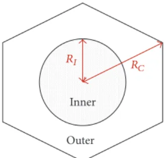
Inner Outer
RI R
C
Figure 1: Inner and outer sections of a cell.
designed for single-carrier systems [38] such as proportional fair scheduler [21, 22], temporal fair scheduler [24], and max-weight scheduler [39]. Reference [38] presents existing work on how single-carrier scheduling algorithms can be adapted to multicarrier environments including OFDM-based LTE networks. Multicarrier systems have their own requirements; for example, a user may have to use the same adaptive modulation and coding scheme on different carriers [29] or a user should be assigned consecutive carriers rather than an arbitrary subset of carriers [40]. These further requirements are known to give rise to complications in multicarrier adaptation [38]. The adaptation of the proposed single-carrier multicell scheduler to multicarrier networks such as LTE-A is deliberately left for future research.
The paper is organized as follows. We present the pro-posed multicell architecture along with the descriptions of cell muting patterns and pattern set construction algorithms in Section 2. The two forms of fairness criteria that we employ as well as the two-level scheduler proposed to satisfy both criteria are presented in Section 3. We validate the effectiveness of the proposed approach in Section 4. Finally, we draw a conclusion.
2. Proposed Multicellular Architecture
2.1. Cells and Users. We consider the downlink of a
time-slotted single-carrier frequency reuse 1 unsectored cellular network (CN) with bandwidth BW where the time slots are
indexed by1 ≤ 𝜏 < ∞. We assume that each cell is divided
into inner and outer sections; see Figure 1 for a cell with cell
radius𝑅𝐶and inner section radius𝑅𝐼. Let𝐶𝑖,𝑖 = 1, 2, . . . , 𝐾,
denote cell𝑖 in the CN where 𝐾 is the total number of cells.
Let BS𝑖denote the base station located in𝐶𝑖. Also let𝐼𝑖and
𝑂𝑖denote the inner and outer sections of𝐶𝑖, respectively. We
let𝑁 denote the total number of users in the network and let
𝑁𝑖,𝑁𝑖𝐼, and𝑁𝑖𝑂denote the number of users associated with
cell𝐶𝑖and with sections𝐼𝑖 and𝑂𝑖, respectively. The cell or
section association of a given user is assumed to be a priori
known throughout this paper. Obviously,𝑁𝑖= 𝑁𝑖𝐼+ 𝑁𝑖𝑂and
𝑁 = ∑𝑖𝑁𝑖. Let𝑈𝑖,𝑗𝐼, 𝑗 = 1, 2, . . . , 𝑁𝑖𝐼and𝑈𝑖,𝑗𝑂,𝑗 = 1, 2, . . . , 𝑁𝑖𝑂
denote the user𝑗 associated with 𝐼𝑖and𝑂𝑖, respectively. We
assume all users are persistent; that is, they always have data to
receive. For a given time slot𝜏, the cell 𝐶𝑖is active (unmuted)
if its BS𝑖 is transmitting. Otherwise,𝐶𝑖is said to be muted.
When𝐶𝑖is active and BS𝑖is transmitting to a user in𝐼𝑖, then
--O1 O2 O3 O4 O5 O6 O7 O8 O9 I1 I2 I3 I4 I5 I6 I7 I8 I9 P1 P2 P3 P4
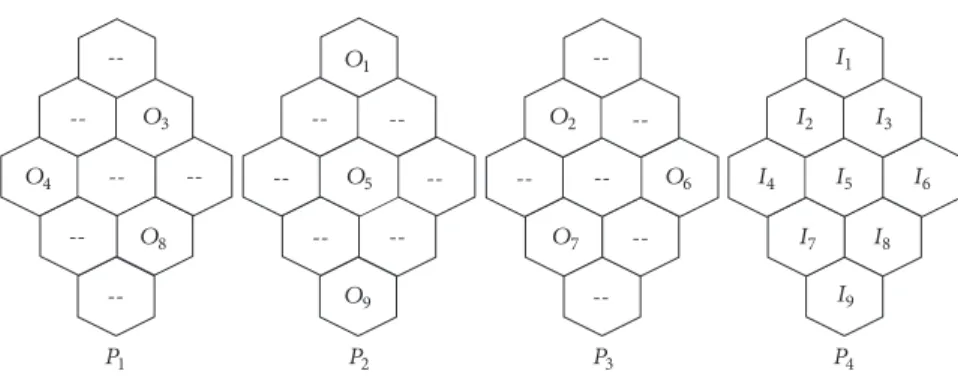
Figure 2: EPS-3 for the 9-cell CN:𝑃1= {𝑂3, 𝑂4, 𝑂8}, 𝑃2= {𝑂1, 𝑂5, 𝑂9}, 𝑃3= {𝑂2, 𝑂6, 𝑂7}, and 𝑃4= {𝐼1, 𝐼2, . . . , 𝐼9}.
2.2. Cell Muting Patterns. A cell muting or transmission
pattern (or pattern in short) is defined as a subset of the set of all sections in the CN satisfying the following two properties: (i) Patterns are noise-limited as opposed to being interference-limited; that is, the elements of a pattern can be activated simultaneously without the associ-ated base stations creating destructive interference on users associated with other active cells. Obviously, when a pattern is selected by the scheduler, all cells which do not have any inner or outer sections in that chosen pattern would be muted.
(ii) Patterns are maximal; that is, a pattern cannot be included in another pattern with larger cardinality. Obviously, a pattern is governed by the geometry of the CN, the power levels used by a BS for transmitting to inner and outer section users, and the definition of destructive interference.
In this paper, patterns are constructed on the basis of an underlying fractional frequency reuse-𝑛- (FFR-𝑛-) type CN; see [41, 42]. In our proposed architecture, the entire bandwidth BW of the frequency reuse 1 system is dynamically shared by the available patterns in time and not in frequency, by means of dynamically muting all but one pattern at a given time slot. Deployment of a general FFR-𝑛 system with
𝑛 = 𝑥2 + 𝑥𝑦 + 𝑦2 for some nonnegative integers 𝑥 and
𝑦 can provide 𝑀 = 𝑛 + 1 patterns for 𝑥, 𝑦 ≥ 1 [5]. We
call the set of𝑛 + 1 patterns an Essential Pattern Set
(EPS-𝑛) for the associated FFR-𝑛 system. Among the patterns in ESP-𝑛, except one transmission pattern which consists of all
inner sections in the network, there are𝑛 patterns each of
which consists of a number of outer sections in the network.
We call all such𝑛 patterns a Mother Pattern Set (MPS-𝑛).
As an example, Figure 2 illustrates ESP-3 which consists of four patterns in a 9-cell CN. Here, MPS-3 denotes the set
{𝑃1, 𝑃2, 𝑃3}.
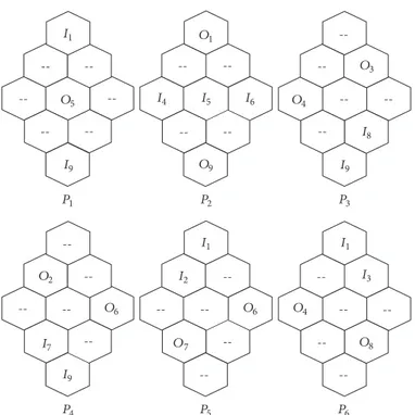
On the other hand, a general pattern set (GPS) is an arbitrary collection of patterns in which each section in the CN is an element of at least one pattern. It is clear that EPS-𝑛 is a GPS. The Universal Pattern Set (UPS) is the set of all possible patterns. Obviously, GPSs are subsets of the UPS. A pattern is said to be active at a given slot if all the sections included in the pattern are active. A section may be included in multiple patterns for a GPS. However, for EPS-𝑛, the patterns are
mutually exclusive. Figure 3 illustrates a sample GPS for the
9-cell CN; note that𝐼9is an element of the three patterns𝑃1,
𝑃3, and𝑃4for this sample GPS.
2.3. General Pattern Set Construction Mechanism. In this
sec-tion, we propose an algorithm to construct a GPS which can effectively be used in multicell networks. For this purpose,
let the operator←→ represent the interference relationship in𝑛
an FFR-𝑛 system with 𝑋 ←→ 𝑌 implying the activation of𝑛
sections𝑋 and 𝑌 causing destructive interference of 𝑋 on 𝑌
and vice versa. In the lack of destructive interference between
the two associated cells, we say𝑋 𝑌. We assume that the𝑛
interference is not destructive if its power is much lower (e.g., 5 times) than the noise power. The interference relationship
which holds for any two given sections𝑋 and 𝑌 depends on
the following two parameters:
(i) The physical distance between the BSs with which
sections𝑋 and 𝑌 are associated
(ii) The transmission power levels assigned to inner and outer section users.
In order to quantify interference between two sections, we make use of the mother patterns in an FFR-𝑛 system. Let
𝐷𝑛 denote the distance between the centers of the nearest
active cells in the patterns of MPS-𝑛. According to [5], we
have𝐷𝑛= 𝑅𝐶√3𝑛. Let us denote by 𝑑𝑖,𝑗the distance between
the centers of𝐶𝑖and𝐶𝑗. Consequently, we have the following
interference identities in an FFR-𝑛 system:
𝑂𝑖←→ 𝑂𝑛 𝑗 iff𝑑𝑖,𝑗< 𝐷𝑛, (1)
𝐼𝑖←→ 𝑂𝑛 𝑗 iff 𝑑𝑖,𝑗< 𝐷𝑛, (2)
𝐼𝑖 𝐼𝑛 𝑗 ∀𝑖, 𝑗. (3)
Moreover, we consider different fixed downlink power levels for inner and outer section users, designed in a way that
(1)–(3) hold. We note that, ∀𝑖 : 𝐼𝑖 ←→ 𝑂𝑛 𝑖 based on (2),
meaning that at most one section per cell can be active at a time slot. The following theorem (given without a proof since it is relatively straightforward) provides the necessary and sufficient conditions for a set of sections to constitute a pattern in an associated FFR-𝑛 CN with 𝐾 cells.
---- ---- ---- --O1 O3 O4 O5 O9 I1 I4 I5 I6 I8 I9 I9 P1 P2 P3 P6 P4 P5 O2 O4 O6 O6 O7 O8 I1 I1 I2 I3 I7 I9
Figure 3: A sample GPS with 6 patterns for the 9-cell CN:𝑃1= {𝐼1, 𝐼9, 𝑂5}, 𝑃2 = {𝐼4, 𝐼5, 𝐼6, 𝑂1, 𝑂9}, 𝑃3= {𝐼8, 𝐼9, 𝑂3, 𝑂4}, 𝑃4= {𝐼7, 𝐼9, 𝑂2, 𝑂6}, 𝑃5= {𝐼1, 𝐼2, 𝑂6, 𝑂7}, and 𝑃6= {𝐼1, 𝐼3, 𝑂4, 𝑂8}.
Theorem 1. A set of sections 𝑃 ̸= ⌀ amounts to a pattern if
and only if (a)∀𝑖, 𝑗 : 𝑂𝑖←→ 𝑂𝑛 𝑗, 𝑂𝑖∈ 𝑃 ⇒ 𝑂𝑗∉ 𝑃, (b)∀𝑖, 𝑗 : 𝑂𝑖←→ 𝐼𝑛 𝑗, 𝑂𝑖∈ 𝑃 ⇒ 𝐼𝑗∉ 𝑃, (c)∀𝑖, 𝑗 : 𝐼𝑖←→ 𝑂𝑛 𝑗, 𝐼𝑖∈ 𝑃 ⇒ 𝑂𝑗∉ 𝑃, (d)∀𝑖 : 𝐼𝑖∉ 𝑃 ⇒ ∃𝑘 : 𝑂𝑘 ←→ 𝐼𝑛 𝑖, 𝑂𝑘∈ 𝑃, (e)∀𝑖 : 𝑂𝑖 ∉ 𝑃 ⇒ ({∃𝑘 : 𝑂𝑘 ←→ 𝑂𝑛 𝑖, 𝑂𝑘 ∈ 𝑃} or {∃𝑘 : 𝐼𝑘←→ 𝑂𝑛 𝑖, 𝐼𝑘∈ 𝑃}).
In Theorem 1, the first three conditions are required for a pattern to be noise-limited whereas the remaining two conditions are required for a pattern to be maximal. One straightforward way to construct all transmission patterns (UPS) is an Exhaustive Search (ES) among all possible sets
of sections of cardinality3𝐾since each cell’s inner section or
outer section is included in a given set or not, leading to three
possibilities for each cell and there are𝐾 such cells. In the
ES method, all of these sets are generated first; then, using Theorem 1, one can check whether each set of sections is a pattern or not. Consequently, in order to check the validity of all the generated sets of sections, the ES method requires
O(3𝐾) steps.
In this paper, we propose a novel algorithm with reduced computational complexity (compared to ES) to construct a
GPS using MPS-𝑛. For this purpose, we let {𝑃∗
𝑚}𝑛𝑚=1 be the
patterns of MPS-𝑛. Also, let 𝑆𝑚
𝑘, 𝑘 = 1, 2, . . . , 2𝑄𝑚 denote
the subset 𝑘 of the set of sections included in 𝑃𝑚∗, where
𝑄𝑚= |𝑃𝑚∗| denotes the number of sections included in 𝑃𝑚∗. For
convenience, let𝑆𝑚1 = 0 and 𝑆𝑄𝑚𝑚 = 𝑃𝑚∗for each𝑚. Algorithm 1
proposes a method to generate a GPS using MPS-𝑛 for an
arbitrary value of𝑛. Figure 4 illustrates the working principle
of Algorithm 1 for𝑛 = 3. In Figure 4(a), one of the mother
patterns in the FFR-3 system is depicted. Figure 4(b) depicts one of the subsets of that mother pattern. Due to interference, neither the inner nor the outer sections of the shadowed cells
can be a member of the new pattern𝑉 in Figure 4(c) based
on (1) and (2). In Figure 4(d), inner sections of the remaining
cells are added to the pattern𝑉 to attain maximality based
on (3). It is clear that EPS-𝑛 is a subset of the pattern set constructed by this algorithm. This is because (i) the set of all inner sections is obtained as a pattern when we start from
the subset𝑆𝑚1 for any𝑚 and (ii) 𝑃𝑚∗is obtained by Algorithm 1
when𝑆𝑚𝑄
𝑚is used in the inner loop for every𝑚. According to
the definition, the collection of all of these patterns is EPS-𝑛. Next, we present Theorem 2 along with its proof showing that the pattern set produced by Algorithm 1 is indeed a GPS.
Theorem 2. The pattern set produced by Algorithm 1 is a GPS. Proof. We need to show that the elements of the pattern
set produced by Algorithm 1 are noise-limited and maximal and moreover each section in the CN is an element of at least one pattern in the pattern set. It is clear that all the
patterns are noise-limited due to the way a new pattern,𝑉,
is generated by Algorithm 1. This is because (i)𝑆𝑚𝑘 is
noise-limited since ∀𝑘, 𝑚 : 𝑆𝑚𝑘 ⊂ 𝑃𝑚∗ and 𝑃𝑚∗ is noise-limited
for every 𝑚 and (ii) line (5) of the algorithm ensures that
any added inner section to 𝑆𝑚𝑘 does not make destructive
interference. On the other hand, assume at least one of the generated patterns is not maximal meaning that we can at
Input: MPS-𝑛 Output: GPS (1) GPS ← ⌀ (2) for 𝑚 = 1 to 𝑛 step (1) do (3) for 𝑘 = 1 to 2|𝑃𝑚∗|do (4) 𝑉 ← 𝑆𝑚 𝑘
(5) Add to𝑉 all the inner sections which do not interfere with the outer sections in 𝑉. (6) if 𝑉 ∉ GPS then
(7) Add𝑉 to the GPS. (8) end if
(9) end for (10) end for
Algorithm 1: Constructing a GPS using MPS-𝑛.
--O3 O4 O8 (a) O4 O8 (b) O4 O8 (c) --O4 O8 I1 I3 (d) Figure 4: Steps to construct a transmission pattern from a mother pattern in an FFR-3 system.
least add one other section (say section𝑋) to it, while it
remains noise-limited. Clearly, section𝑋 cannot be an inner
section, because Algorithm 1 adds all possible inner sections
(line(5) of Algorithm 1). On the other hand, 𝑋 cannot be an
outer section because of assuming that𝑋 is the outer section
of cell𝑌 with the inner section 𝑍. If adding 𝑋 would not cause
destructive interference, then adding𝑍 also would not cause
destructive interference. However, this contradicts with the
way the algorithm works (line(5) of Algorithm 1). To show
that each section is an element of at least one pattern, recall that patterns which belong to MPS-𝑛 are among the generated patterns and each of the outer sections is an element of an individual MPS. Moreover, the set of all inner sections is
obtained as a pattern when we start from the subset𝑆𝑚1 for
any𝑚. This concludes the proof.
We now elaborate on the computational aspects of the GPS construction algorithm that we have proposed. The outer
loop of Algorithm 1 requires𝑛 iterations and the inner loop
requires approximately2⌈𝐾/𝑛⌉iterations. To see this, there are
𝑛 mother patterns, namely, {𝑃∗
𝑚}𝑛𝑚=1, and each mother pattern
𝑃∗
𝑚 consists of approximately|𝑃𝑚∗| ≈ ⌈𝐾/𝑛⌉ outer sections,
so each inner loop will be executed approximately 2⌈𝐾/𝑛⌉
times. Therefore, the total number of required iterations is
O(2⌈𝐾/𝑛⌉𝑛) which is substantially less than that of the ES
method. Moreover, the per-iteration computational load of Algorithm 1 is less than that of ES. However, recall that this
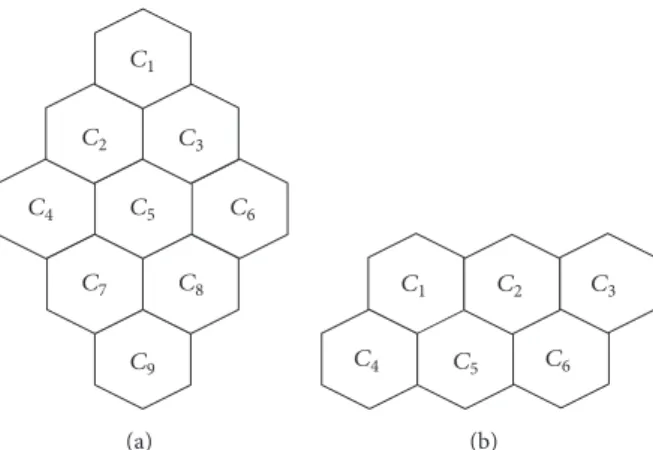
GPS is only a subset of the UPS and there may be patterns in the UPS that cannot be constructed by the proposed algorithm. To evaluate the pattern construction capability of Algorithm 1, we consider two different CNs illustrated in Figure 5 depicting (a) 9-cell and (b) 6-cell scenarios, which will be used in numerical examples. We use the FFR-3 interference relationships and subsequently MPS-3 as input to the proposed algorithm. The ES and Algorithm 1 are run for each of the two scenarios and the patterns constructed by each method are presented in Tables 1 and 2, respectively, for the 9-cell and 6-cell scenarios. We observe that ES generates the UPS with cardinality 42 and cardinality 13, whereas Algorithm 1 constructs 22 and 10 patterns, respectively, for the 9-cell and 6-cell scenarios. Although the proposed algorithm cannot construct the UPS, we will later show through numerical examples that the network performance obtained by the GPS produced by the proposed algorithm is only slightly inferior to that attained by that of the UPS.
3. The Proposed Multicell Scheduler
In this section, we assume that the pattern set{𝑃𝑚}𝑀𝑚=1is a
priori given whether being EPS-𝑛, or the UPS if available, or the GPS produced by the algorithm presented in the previous
section, or any other GPS. At a decision epoch𝜏, the NLS
decides to activate one of the available patterns, say𝑃𝑚∗(𝜏),
C1 C2 C3 C4 C5 C6 C7 C8 C9 (a) C1 C2 C3 C4 C5 C6 (b)
Figure 5: Two different scenarios: (a) 9-cell CN; (b) 6-cell CN.
patterns. How this decision is to be made will be discussed in the sequel.
3.1. Per-Pattern and Per-User Temporal Shares. Let𝐴𝑚,𝑎𝑖,𝑗𝐼,
and𝑎𝑂𝑖,𝑗denote the long-term temporal (or equivalently
air-time) share of pattern𝑃𝑚, user𝑈𝑖,𝑗𝐼, and user𝑈𝑖,𝑗𝑂, respectively:
𝐴𝑚= lim 𝑡→∞ 1 𝑡 𝑡 ∑ 𝜏=1 1 {𝑚∗(𝜏) = 𝑚} 𝑎𝑖,𝑗𝐼 = lim𝑡→∞1𝑡∑𝑡 𝜏=11 {user 𝑈 𝐼 𝑖,𝑗is scheduled at slot 𝜏} 𝑎𝑖,𝑗𝑂 = lim 𝑡→∞ 1 𝑡 𝑡 ∑ 𝜏=1
1 {user 𝑈𝑖,𝑗𝑂 is scheduled at slot 𝜏} ,
(4)
where1{⋅} denotes the conventional indicator function which
is either one or zero depending on whether the argument is
true or not, respectively. Similarly, let𝐴𝐼𝑖,𝐴𝑂𝑖, and𝐴𝐶𝑖 denote
the long-term air-time share of section𝐼𝑖, section𝑂𝑖, and cell
𝐶𝑖, respectively. Mathematically, 𝐴𝐼𝑖= lim 𝑡→∞ 1 𝑡 𝑡 ∑ 𝜏=11 {𝐼𝑖∈ 𝑃𝑚 ∗(𝜏)} 𝐴𝑂𝑖 = lim 𝑡→∞ 1 𝑡 𝑡 ∑ 𝜏=1 1 {𝑂𝑖∈ 𝑃𝑚∗(𝜏)} 𝐴𝐶𝑖 = 𝐴𝐼𝑖+ 𝐴𝑂𝑖. (5)
We introduce positive (target) scheduling weights{𝑤𝑚}𝑀𝑚=1
for patterns {𝑃𝑚}𝑀𝑚=1 satisfying ∑𝑚𝑤𝑚 = 1. The target
scheduling weight𝑤𝑚is the long-term target average
proba-bility that pattern𝑃𝑚is selected by the scheduler. Note that
use of scheduling weight{𝑤𝑚}𝑀𝑚=1 by the scheduler should
give rise to𝐴𝑚 = 𝑤𝑚, ∀𝑚. In this case, the system is said
to be interpattern weighted temporal fair with respect to
the weights {𝑤𝑚}𝑀𝑚=1. In the specific case of𝑤𝑚 = 1/𝑀,
the system is called interpattern temporal fair. Similarly, we
introduce target positive scheduling weights {𝑤𝑖,𝑗𝐼}𝑁𝑖𝐼
𝑗=1 and
{𝑤𝑖,𝑗𝑂}𝑁𝑖𝑂
𝑗=1 for user 𝑈𝑖,𝑗𝐼 and user 𝑈𝑖,𝑗𝑂, respectively, satisfying
∑𝑗𝑤𝐼
𝑖,𝑗 = 1 and ∑𝑗𝑤𝑂𝑖,𝑗 = 1 for each of the cells 𝐶𝑖. We
remark that the use of user scheduling weights{𝑤𝐼𝑖,𝑗}𝑁𝑖𝐼
𝑗=1and
{𝑤𝑂
𝑖,𝑗}𝑁
𝑂 𝑖
𝑗=1 leads to𝑎𝑖,𝑗𝐼 = 𝐴𝐼𝑖𝑤𝑖,𝑗𝐼, ∀𝑗, for any section 𝐼𝑖 and
𝑎𝑂
𝑖,𝑗 = 𝐴𝑂𝑖𝑤𝑂𝑖,𝑗, ∀𝑗, for any section 𝑂𝑖. In this case we have
intrasection weighted temporal fairness in sections 𝐼𝑖 and
𝑂𝑖, respectively, with respect to the weights {𝑤𝑖,𝑗𝐼}𝑁𝑖𝐼
𝑗=1 and
{𝑤𝑂
𝑖,𝑗}𝑁
𝑂 𝑖
𝑗=1. In this paper, we only consider ordinary intrasection
temporal fairness which leads to the following two identities:
𝑤𝐼𝑖,𝑗= 1 𝑁𝐼 𝑖 , 1 ≤ 𝑗 ≤ 𝑁𝑖𝐼, 𝑤𝑂 𝑖,𝑗=𝑁1𝑂 𝑖 , 1 ≤ 𝑗 ≤ 𝑁𝑖𝑂. (6)
In case when 𝑁𝑖𝐼 or 𝑁𝑖𝑂 is zero, no per-user scheduling
weights are assigned for that particular section. Moreover, no downlink transmission would take place due to the lack of a user in that section even if the included pattern is selected for transmission. Therefore, the only unknowns to the scheduler in the numerical examples of the current study are the per-pattern weights. Once the weights are decided, then the following identities immediately hold:
𝐴𝐼𝑖 = ∑𝑀 𝑚=1 𝑤𝑚𝑒𝑚,𝑖, 𝑎𝐼𝑖,𝑗= 𝐴𝐼𝑖 𝑁𝐼 𝑖 , (7) 𝐴𝑂𝑖 = ∑𝑀 𝑚=1 𝑤𝑚𝑓𝑚,𝑖, 𝑎𝑂𝑖,𝑗= 𝐴𝑂𝑖 𝑁𝑂 𝑖 , (8)
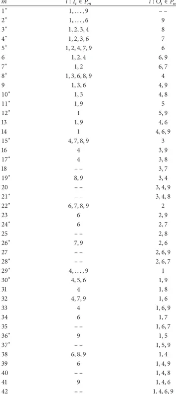
Table 1: The UPS with 42 patterns for the 9-cell network. The patterns labeled with∗ are constructed by Algorithm 1.
𝑚 𝑖 : 𝐼𝑖∈ 𝑃𝑚 𝑖 : 𝑂𝑖∈ 𝑃𝑚 1∗ 1, . . . , 9 – – 2∗ 1, . . . , 6 9 3∗ 1, 2, 3, 4 8 4∗ 1, 2, 3, 6 7 5∗ 1, 2, 4, 7, 9 6 6 1, 2, 4 6, 9 7∗ 1, 2 6, 7 8∗ 1, 3, 6, 8, 9 4 9 1, 3, 6 4, 9 10∗ 1, 3 4, 8 11∗ 1, 9 5 12∗ 1 5, 9 13 1, 9 4, 6 14 1 4, 6, 9 15∗ 4, 7, 8, 9 3 16 4 3, 9 17∗ 4 3, 8 18 – – 3, 7 19∗ 8, 9 3, 4 20 – – 3, 4, 9 21∗ – – 3, 4, 8 22∗ 6, 7, 8, 9 2 23 6 2, 9 24∗ 6 2, 7 25 – – 2, 8 26∗ 7, 9 2, 6 27 – – 2, 6, 9 28∗ – – 2, 6, 7 29∗ 4, . . . , 9 1 30∗ 4, 5, 6 1, 9 31 4 1, 8 32 4, 7, 9 1, 6 33 4 1, 6, 9 34 6 1, 7 35 – – 1, 6, 7 36∗ 9 1, 5 37∗ – – 1, 5, 9 38 6, 8, 9 1, 4 39 6 1, 4, 9 40 – – 1, 4, 8 41 9 1, 4, 6 42 – – 1, 4, 6, 9 where 𝑒𝑚,𝑖 ≜ 1{𝐼𝑖 ∈ 𝑃𝑚} and 𝑓𝑚,𝑖 ≜ 1{𝑂𝑖 ∈ 𝑃𝑚}. In
the next subsection, we focus on methods of obtaining these weights leading to two different forms of temporal fairness being sought in the CN.
3.2. Temporal Fairness Criteria. In this paper, we consider
two different TF criteria for the multicell CN for which
Table 2: The UPS with 13 patterns for the 6-cell network. The patterns labeled with∗ are constructed by Algorithm 1.
𝑚 𝑖 : 𝐼𝑖∈ 𝑃𝑚 𝑖 : 𝑂𝑖∈ 𝑃𝑚 1∗ – – 1, 6 2∗ – – 2, 4 3∗ – – 3, 5 4∗ 1, . . . , 6 – – 5∗ 2, 3, 6 4 6∗ 4 2 7∗ 3 5 8∗ 1, 4, 5 3 9∗ 3, 6 1 10 – – 3, 4 11 – – 4, 6 12∗ 1, 4 6 13 – – 1, 3
the per-pattern weights can easily be obtained at reasonable computational complexity. The first TF criterion is the so-called Intersection Proportional Temporal Fairness (IS-PTF) in which the CN is intercell temporal fair one but an inner section of each cell receives a temporal share proportional to the temporal share of the outer section of the same cell using the same network-wide proportionality constant.
Mathematically, 𝐴𝐶𝑖 = 𝐴𝐶𝑗, 1 ≤ 𝑖, 𝑗 ≤ 𝐾, and 𝐴𝐼𝑖 =
𝑑𝐴𝑂𝑖, 1 ≤ 𝑖 ≤ 𝐾, hold for a fairness proportionality constant
𝑑 to be chosen by the network operator. As a matter of fact,
employing𝑑 > 1 causes the inner sections to be scheduled
more often than the outer sections and vice versa for the case 0 < 𝑑 < 1. It is clear that IS-PTF cannot be achieved for some general pattern sets such as GPS of Figure 3. However, as stated in the theorem below, IS-PTF is achievable when EPS-𝑛 is used as the pattern set.
Theorem 3. With EPS-𝑛 used as the pattern set, IS-PTF is achieved by the following choice of weights:
𝑤𝑖= 𝑑 + 𝑛1 1 ≤ 𝑖 ≤ 𝑛,
𝑤𝑛+1= 𝑑
𝑑 + 𝑛,
(9)
where𝑀 = 𝑛 + 1 and the pattern 𝑃𝑀is the set of all inner sections of the CN; that is,𝑃𝑀= ⋃𝐾𝑖=1𝐼𝑖.
Proof. We note that EPS-𝑛 = MPS-𝑛 ∪ 𝑃𝑀 and 𝐴𝑚, 1 ≤
𝑚 ≤ 𝑛, and 𝐴𝑀are the temporal shares of𝑚th individual
MPS-𝑛 and 𝑃𝑀, respectively. Furthermore, the scheduler can
guarantee that𝐴𝑚= 𝑤𝑚, 1 ≤ 𝑚 ≤ 𝑛 and 𝐴𝑀= 𝑤𝑀. Patterns
in MPS-𝑛 are mutually exclusive; thus for each section 𝑂𝑖
there is only one index𝑚, 1 ≤ 𝑚 ≤ 𝑛, such that 𝐴𝑂𝑖 = 𝑤𝑚.
Furthermore,∀𝑖 : 𝐴𝐼𝑖 = 𝑤𝑀. We thus conclude that, for all
𝑖, there exists 𝑚, 1 ≤ 𝑚 ≤ 𝑛, such that 𝐴𝐶
𝑖 = 𝑤𝑚 + 𝑤𝑀.
Recall that intercell fairness requires∀𝑚1, 𝑚2, 1 ≤ 𝑚1, 𝑚2 ≤
𝑛 : 𝑤𝑚1 + 𝑤𝑀 = 𝑤𝑚2 + 𝑤𝑀 which in turn implies that
using intersection fairness we have∀𝑚, 1 ≤ 𝑚 ≤ 𝑛 : 𝑤𝑀 =
𝑑𝑤𝑚 = 𝑑𝑤. Finally, the pattern weights sum to unity; that
is,∑𝑛𝑚=1𝑤𝑚 + 𝑤𝑀 = 1. Therefore, 𝑛𝑤 + 𝑑𝑤 = 1 which
implies that∀𝑚, 1 ≤ 𝑚 ≤ 𝑛 : 𝑤𝑚 = 𝑤 = 1/(𝑑 + 𝑛) and
𝑤𝑀= 𝑤𝑛+1= 𝑑/(𝑑 + 𝑛).
For the special case of EPS-3, there are𝑀 = 4 patterns
depicted in Figure 2 where the corresponding weights are
𝑤1= 𝑤2= 𝑤3= 1/(𝑑 + 3) and 𝑤4= 𝑑/(𝑑 + 3).
Although IS-PTF criterion guarantees equal user tem-poral shares within each section, it does not seek network-wide fairness among all the network users. That is why IS-PTF does not take into account the number of users located
in each section for obtaining pattern weights{𝑤𝑚}𝑀𝑚=1. As a
result, using IS-PTF along with unbalanced user distribution may lead to unequal temporal share for the users located in different sections of the network. The second TF criterion we study in this paper is max-min temporal fairness (MMTF)
for which the pattern weights{𝑤𝑚}𝑀𝑚=1are selected so that
the minimum user temporal share in the network is maxi-mized. Thus, MMTF is a network-wide fairness criterion. The MMTF is easily shown to be reducible to the following linear program: maximize 𝑧,𝑤1,𝑤2,...,𝑤𝑀 𝑧 subject to: 𝑧 ≤ ∑ 𝑀 𝑚=1𝑤𝑚𝑒𝑚,𝑖 𝑁𝐼 𝑖 , 𝑧 ≤ ∑ 𝑀 𝑚=1𝑤𝑚𝑓𝑚,𝑖 𝑁𝑂 𝑖 1 ≤ 𝑖 ≤ 𝐾, 𝑀 ∑ 𝑚=1 𝑤𝑚= 1, 𝑤𝑚≥ 0 1 ≤ 𝑚 ≤ 𝑀, (10)
where𝑧 is the minimum network-wide user temporal share.
The convexity of optimization problem (10) follows from the linearity of the objective function and constraints [43]. It is not difficult to show that for a given GPS this linear program has at least one solution and in the case of a
nonunique solution, the objective function value, that is,𝑧,
is the same for all the solutions due to the convexity of the program. While there is no general closed form solution for MMTF, Theorem 4 provides a closed form solution when the patterns are mutually exclusive (e.g., EPS-𝑛). When patterns are not mutually exclusive, there are numerous efficient numerical methods including simplex and interior point algorithms via which one can obtain a solution for MMTF with reasonable effort.
Theorem 4. If the patterns are mutually exclusive, the solution to the MMTF problem is unique and one has
𝑤∗ 𝑚= ∑𝑀𝑛𝑚 𝑙=1𝑛𝑙 1 ≤ 𝑚 ≤ 𝑀, 𝑧∗= 1 ∑𝑀𝑙=1𝑛𝑙, (11)
where𝑛𝑚 denotes the number of users in the most crowded section of pattern𝑚; that is, 𝑛𝑚= max𝑖{𝑁𝑖𝐼𝑒𝑚,𝑖, 𝑁𝑖𝐼𝑓𝑚,𝑖}𝐾𝑖=1. Proof. Let {𝑤𝑚∗}𝑀𝑚=1 and 𝑧∗ denote the solution of MMTF problem (10). Because the patterns are mutually exclusive, each section of the network is covered by one pattern. Therefore, according to (7), the minimum user air-time in
pattern 𝑚 is 𝑤∗𝑚/𝑛𝑚. In other words, users in the most
crowded section of pattern𝑚 have the minimum air-time
share among all the users in that pattern. The claim is that the
value of𝑤∗𝑚/𝑛𝑚is the same for every𝑚. Let us assume that
the claim is not correct. Therefore, if the user with minimum
air-time share is in pattern𝑚, then there exists at least one
𝑚 for which𝑤∗
𝑚/𝑛𝑚 < 𝑤∗𝑚/𝑛𝑚. It is clear that we can
increase the minimum user air-time share in the network
by decreasing𝑤𝑚∗and increasing 𝑤∗𝑚. Therefore,𝑤𝑚∗ and
𝑤𝑚∗are not optimal which is contradiction and the claim is
correct. We can conclude that∀𝑚 : 𝑧∗ = 𝑤∗𝑚/𝑛𝑚. On the
other hand, we know that∑𝑚𝑤𝑚= 1. Eventually, we can find
the unique solution of MMTF problem, that is,{𝑤∗𝑚}𝑀𝑚=1and
𝑧∗, by solving the system of these𝑀 + 1 independent linear
equations as given in (11).
We should note that, unlike IS-PTF, the MMTF problem always has a solution for any GPS. We also note that to solve
the MMTF problem each BS𝑖is required to send the values
𝑁𝐼
𝑖 and 𝑁𝑖𝑂 to the NLS which subsequently solves linear
program (10) to obtain the per-pattern scheduling weights
{𝑤𝑚}𝑀
𝑚=1. Note that it is not necessary to solve the MMTF
problem at each time slot. Instead, the MMTF problem can be solved when the number of users in any one of the sections of the CN changes. Alternatively, the MMTF linear program can be solved if the change in the number of users in the individual sections of the CN is substantial and the previous solutions’ weights can be used until such a substantial change. It is clear that this alternative mechanism may reduce the computational burden on the NLS.
For the two fairness criteria studied in this paper, namely, IS-PTF and MMTF, we have described methods by which
the scheduling weights{𝑤𝑚}𝑀𝑚=1are obtained. Exploration of
other temporal fairness criteria are left for future research. In the next subsection, we are going to introduce a two-level scheduler that uses these scheduling weights so as to make opportunistic fair decisions to select patterns at the network-level and also users belonging to these patterns at the cell-level.
3.3. Two-Level Opportunistic Scheduler. In this section, we
assume that the scheduling weights{𝑤𝑚}𝑀𝑚=1, {𝑤𝑖,𝑗𝐼}𝑁𝐼𝑖
𝑗=1, and
{𝑤𝑂
𝑖,𝑗}𝑁
𝑂 𝑖
𝑗=1are a priori given. Although the per-user scheduling
weights in the current study are based on the identities (6), the proposed two-level scheduler described later in this section works for arbitrary per-user scheduling weights
{𝑤𝐼 𝑖,𝑗}𝑁 𝐼 𝑖 𝑗=1 and {𝑤𝑂𝑖,𝑗}𝑁 𝑂 𝑖
𝑗=1. Subsequently, we introduce a credit
parameter𝑏𝑖,𝑗𝐼 for each inner section user 𝑈𝑖,𝑗𝐼 and another
credit parameter 𝑏𝑖,𝑗𝑂 for each outer section user 𝑈𝑖,𝑗𝑂 with
at BS𝑖. We also introduce a credit parameter 𝐵𝑚 for each
pattern𝑃𝑚 maintained by the NLS. The initial values of all
these credit parameters are set to zero at the beginning of network operation. We also define the instantaneous spectral
efficiency (SE) 𝑟𝑖,𝑗𝐼(𝜏) (𝑟𝑂𝑖,𝑗(𝜏)) in units of bps/Hz for user
𝑈𝐼
𝑖,𝑗 (𝑈𝑖,𝑗𝑂) at time slot 𝜏. In particular, in our numerical
experiments, we use the Shannon formula
𝑟𝐼𝑖,𝑗(𝜏) = log2(1 + SNR𝐼𝑖,𝑗(𝜏)) ,
𝑟𝑂𝑖,𝑗(𝜏) = log2(1 + SNR𝑂𝑖,𝑗(𝜏)) , (12)
where SNR𝐼𝑖,𝑗(𝜏) and SNR𝑂𝑖,𝑗(𝜏) denote the signal to noise
ratio of users 𝑈𝑖,𝑗𝐼 and 𝑈𝑖,𝑗𝑂, respectively, at slot 𝜏 [44].
Other relationships of SE to the SNR than (12) can also be used. Next, we describe our proposed two-level multicell
scheduling algorithm at a given time slot 𝜏 in a six-step
process.
Step 1. As for the CLS, BS𝑖of each cell𝐶𝑖selects two users
𝑗∗
𝑖,𝐼and𝑗∗𝑖,𝑂from the inner section𝐼𝑖and outer section𝑂𝑖of
the cell, respectively, based on the instantaneous user SEs and per-user credit parameter values as follows:
𝑗𝑖,𝐼∗ = arg max 1≤𝑗≤𝑁𝐼 𝑖 (𝑟𝐼𝑖,𝑗(𝜏) + 𝛼𝑏𝑖,𝑗𝐼) , 𝑗𝑖,𝑂∗ = arg max 1≤𝑗≤𝑁O 𝑖 (𝑟𝑂𝑖,𝑗(𝜏) + 𝛼𝑏𝑖,𝑗𝑂) , (13)
where𝛼 > 0 is an algorithm parameter that we will study in
the numerical examples to be shown to affect the convergence time and the overall network throughput.
Step 2. For each cell, the CLS of cell𝐶𝑖 then nominates the
users𝑗𝑖,𝐼∗ and𝑗∗𝑖,𝑂and the instantaneous per-section SEs of the
sections𝐼𝑖and𝑂𝑖, denoted by
𝑅𝐼𝑖(𝜏) = 𝑟𝑖,𝑗𝐼∗ 𝑖,𝐼(𝜏) , 𝑅𝑂 𝑖 (𝜏) = 𝑟𝑖,𝑗𝑂∗ 𝑖,𝑂(𝜏) , (14)
respectively, if the nominated users were to be served. BS𝑖
then disseminates the values𝑅𝐼𝑖(𝜏) and 𝑅𝑂𝑖 (𝜏) to the NLS.
Step 3. For the pattern selection, in the third step, the NLS
obtains the network-wide SE of pattern𝑃𝑚, denoted by𝑅𝑚(𝜏),
as follows:
𝑅𝑚(𝜏) =∑𝐾
𝑖=1
(𝑅𝐼𝑖(𝜏) 𝑒𝑚,𝑖+ 𝑅𝑂𝑖 (𝜏) 𝑓𝑚,𝑖) , 1 ≤ 𝑚 ≤ 𝑀. (15)
Step 4. The NLS selects the pattern𝑃𝑚∗to be activated based
on the following identity:
𝑚∗= arg max
1≤𝑚≤𝑀 (𝑅𝑚(𝜏) + 𝛽𝐵𝑚) , (16)
where𝛽 is a second algorithm parameter similar to 𝛼 in (13).
Step 5. Once𝑚∗is determined, the per-pattern credit param-eters are updated in the fifth step as follows:
𝐵𝑚= 𝐵𝑚+ 𝑤𝑚− 1 {𝑚 = 𝑚∗} 1 ≤ 𝑚 ≤ 𝑀. (17)
The NLS then sends a message to all CLSs with the informa-tion on which pattern was selected in the current slot.
Step 6. The nominated users in the sections belonging to
the selected pattern𝑃𝑚∗ are scheduled in the current time
slot. Moreover, the credit parameters of users in the sections
belonging to the selected pattern𝑃𝑚∗are updated as follows:
𝑏𝑖,𝑗𝐼 = 𝑏𝑖,𝑗𝐼 + 𝑤𝐼𝑖,𝑗− 1 {𝑗 = 𝑗∗𝑖,𝐼} , ∀𝑗, 𝐼𝑖∈ 𝑃𝑚∗,
𝑏𝑖,𝑗𝑂= 𝑏𝑖,𝑗𝑂+ 𝑤𝑂𝑖,𝑗− 1 {𝑗 = 𝑗∗𝑖,𝑂} , ∀𝑗, 𝑂𝑖∈ 𝑃𝑚∗.
(18) The credit parameters of users in sections that do not reside in the selected pattern are not updated and those sections are not activated in the current slot.
Moreover, one can write the long-term average network
throughput𝑇 as follows:
𝑇 = lim𝑡→∞BW𝑡 ∑𝑡
𝜏=1𝑅𝑚
∗(𝜏) . (19)
3.4. Remarks on the Proposed Algorithm. Per-pattern credit
parameters are updated in (17) and it is obvious that these parameters cannot grow to either plus or minus infinity. This can be observed from the decision made to activate a pattern at the network-level according to (16) which ensures that credit parameters will stay bounded. Bounded credit parameters are indication of satisfaction of desired temporal fairness constraints at the pattern level. Similar conclusions can be drawn for the per-user credit parameters and the satisfaction of desired temporal fairness constraints at the user level. Although we do not have optimality results for the proposed multicell scheduler, we note that the structures of the two TF schedulers NLS in (16) and the CLSs in (13) follow that of the single-cell optimum TF scheduler described in [24]
except that we use fixed coefficients𝛼 and 𝛽 as in [28] instead
of those that decay in time. The purpose of this choice is to satisfy fairness constraints not only in the long-term but also in shorter time scales. Numerical examples will be presented to validate these choices.
The NLS has O(𝑀𝐾) computational complexity and
O(𝑀) storage requirements and presents a scalable solu-tion when compared to existing methods whose complexity
depends on the overall number of users𝑁 in the network.
Due to low communications overhead between the CLSs and the NLS, the proposed method is relatively practical and can be implemented using a sufficiently low-delay backhaul. However, we note that the two-way CLS to NLS commu-nication should be completed before any data transmission can start in the proposed algorithm. For larger slot lengths, this communication delay is less of a problem. However, for shorter slots, inefficiencies due to signaling overhead may be significant. The adaptation of the proposed algorithm to more realistic multicarrier wireless networks with short slots (e.g., LTE-A with subframes of 0.1 ms) is left for future research.
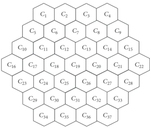
C1 C2 C3 C4 C5 C6 C7 C8 C9 C10 C11 C12 C13 C14 C15 C16 C17 C18 C19 C20 C21 C22 C23 C24 C25 C26 C27 C28 C29 C30 C31 C32 C33 C34 C35 C36 C37
Figure 6: 37-cell cellular network.
4. Numerical Examples
In all the numerical examples, we use one of the 6-cell and 9-cell CNs provided in Figure 5 and an additional 37-cell
CN depicted in Figure 6. The radii parameters 𝑅𝐼 and 𝑅𝐶
are assumed to be0.5 km and 1 km, respectively, for all the
CNs. The system frequency is assumed to be 2 GHz and
BW is set to20 MHz. Noise power spectral density and user
equipment noise figure are assumed to be−174 dBm/Hz and
9 dB, respectively. Transmission power of each BS to the inner and outer users is 30 dBm and 40 dBm, respectively. It is straightforward to show that the choices of transmit
powers and radii parameters𝑅𝐶 and 𝑅𝐼 satisfy (1)–(3) for
𝑛 = 3 which is our focus in this section. The large-scale fading channel coefficients are modeled based on the
COST-231 model as−140.7 − 35.2 log10(𝑑𝑈BS) + Ψ in dB scale, where
𝑑𝑈
BS is the distance between the corresponding user and BS,
and Ψ ∼ 𝑁(0, 𝜎Ψ2) represents the log-normal shadowing
effect. We assume that𝜎Ψ=4 dB. Rayleigh fading model is
adopted for small-scale channel coefficient variations [5]. It is assumed that small-scale fading channel coefficients are fixed during each time slot and vary independently over different time slots (block fading). Also, we assume that shadow fading coefficients are fixed in the duration of 50 consecutive time slots and vary independently otherwise.
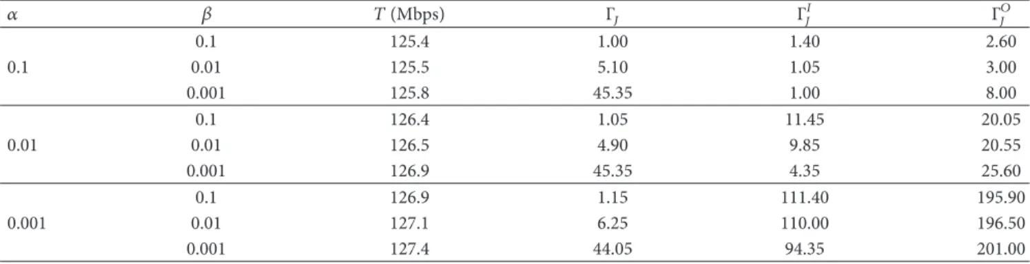
4.1. Study of Scheduler Parameters𝛼 and 𝛽. In this example,
we study the effect of the algorithm parameters 𝛼 and
𝛽 employed through the identities (13) and (16), on the convergence time and long-term network throughput. We assume that the scheduler uses EPS-3 with cardinality 4 in the 9-cell network of Figure 5(a). We employ IS-PTF with the
parameter𝑑 set to unity; that is, we seek ordinary intercell
and intersection fairness in this example. For a given section
𝐼𝑖 (𝑂𝑖), let𝐽𝑖𝐼(𝑡) (𝐽𝑖𝑂(𝑡)) denote Jain’s fairness index for the
temporal shares𝑎𝐼𝑖,𝑗(𝑡) (𝑎𝑖,𝑗𝑂(𝑡)) which are shares of the users
𝑈𝐼
𝑖,𝑗(𝑈𝑖,𝑗𝑂(𝑡)) up to time 𝑡. We refer to [45] for the definition
of Jain’s fairness index. Let us also define the intrasection
fairness index𝐽𝐼(𝑡) = min𝑖𝐽𝑖𝐼(𝑡) (𝐽𝑂(𝑡) = min𝑖𝐽𝑖𝑂(𝑡)) for
inner (outer) sections. Proximity of𝐽𝐼(𝑡) (𝐽𝑂(𝑡)) to unity is
representative of intrasection fairness for the inner (outer)
section users up to time𝑡. Also, let the interpattern fairness
index𝐽(𝑡) be defined by Jain’s fairness index for the individual
per-pattern temporal shares{𝐴𝑚(𝑡)}. Similarly, proximity of
𝐽(𝑡) to unity is representative of interpattern fairness up to
time 𝑡. Furthermore, we note that interpattern fairness is
equivalent to ordinary intercell fairness in this example since
the patterns are mutually exclusive. We assume 𝑁 = 64
uniformly located users in the 9-cell network of Figure 5(a) for each of the 20 simulation instances and for each instance
we run the two-level scheduler for a duration of5 × 106slots
with various choices of𝛼 and 𝛽. In each simulation instance,
we obtain the valuesΓ𝐽andΓ𝐽𝐼(Γ𝐽𝑂), which are defined as the
minimum value of𝑡 such that 𝐽(𝐻𝑡) ≥ 1 − 𝜖 and 𝐽𝐼(𝐻𝑡) ≥
1 − 𝜖 (𝐽𝑂(𝐻𝑡) ≥ 1 − 𝜖), respectively, for a small tolerance
parameter 𝜖 > 0 which is set to 0.05 and for a sampling
parameter𝐻 set to 1000. A relatively large value of Γ𝐽𝐼(Γ𝐽𝑂) is
indicative of longer convergence times and therefore adverse impact on short-term intrasection fairness for inner (outer) section users. On the other hand, a relatively large value of
Γ𝐽is indicative of short-term intercell unfairness. The
steady-state throughput𝑇 and three fairness metrics Γ𝐽,Γ𝐽𝐼, andΓ𝐽𝑂
(average values obtained over the 20 simulation instances) are
tabulated in Table 3 for various choices of𝛼 and 𝛽.
We observe from Table 3 that the particular choice of the
algorithm parameters𝛼 and 𝛽 has only a slight impact on
the overall throughout with slight improvement in𝑇 with
lower choices of𝛼 and 𝛽. On the other hand, when 𝛼 and
𝛽 are decreased, as a penalty, the various fairness indices of interest converge in a slower manner and short-term intercell and intrasection fairness measures are consequently
compromised. In particular, whileΓ𝐽is more sensitive to the
change of𝛽, Γ𝐽𝐼andΓ𝐽𝑂appear to more sensitive to the change
of𝛼. Similar observations are made in other scenarios as well
but are not reported in the current manuscript. As a trade-off between short-term intercell and intrasection fairness and
total network throughput, we fix 𝛼 = 𝛽 = 0.01 in the
remaining numerical examples.
4.2. Comparison of Opportunistic FFR versus Benchmark FFR. The use of the pattern set EPS-3 with the proposed
opportunistic scheduler based on IS-PTF is referred to as opportunistic FFR (OFFR) in this paper. In this example, OFFR uses the IS-PTF formulation with a certain choice
of the parameter𝑑 introduced in (9). In particular, we first
study three different values of the parameter𝑑, namely, 𝑑 =
1/4, 1, 4, and consequently use the per-pattern weights as given in (9). The benchmark system called benchmark FFR (BFFR) splits the BW into four subbands, the bandwidth of
each subband being proportional to𝑤𝑚 for𝑚 ∈ {1, 2, 3, 4}
based on identity (9). The intracell scheduler of BFFR is the same as that of the OFFR. Besides, we note that there is no NLS in BFFR and ICI is handled by static spectrum
partitioning as described above. For each value of 𝑑, we
simulated BFFR and OFFR in both 9-cell and 37-cell CNs for
a total of 400 instances each of which spans106time slots.
Table 3: The average throughput𝑇 and the average of three fairness metrics Γ𝐽,Γ𝐽𝐼, andΓ𝐽𝑂for various values of𝛼 and 𝛽 for the 9-cell CN. 𝛼 𝛽 𝑇 (Mbps) Γ𝐽 Γ𝐼 𝐽 Γ𝐽𝑂 0.1 125.4 1.00 1.40 2.60 0.1 0.01 125.5 5.10 1.05 3.00 0.001 125.8 45.35 1.00 8.00 0.1 126.4 1.05 11.45 20.05 0.01 0.01 126.5 4.90 9.85 20.55 0.001 126.9 45.35 4.35 25.60 0.1 126.9 1.15 111.40 195.90 0.001 0.01 127.1 6.25 110.00 196.50 0.001 127.4 44.05 94.35 201.00 −5 0 5 10 15 20 25 30 35 40 45 0 0.2 0.4 0.6 0.8 1 Em pi ri cal CD F Inner d = 4 Inner d = 1 Inner d = 1/4 Outer d = 4 Outer d = 1 Outer d = 1/4 User throughput gains GI
i,j, GOi,j
(a) 9-cell scenario
0 5 10 15 20 25 30 35 40 45 0 0.2 0.4 0.6 0.8 1 Em pi ri cal CD F Inner d = 4 Inner d = 1 Inner d = 1/4 Outer d = 4 Outer d = 1 Outer d = 1/4 User throughput gains GI
i,j, Gi,jO
(b) 37-cell scenario
Figure 7: Empirical CDF of the users throughput gains𝐺𝐼𝑖,𝑗and𝐺𝑂𝑖,𝑗for𝑁 = 64 for three different values of 𝑑 in 9-cell and 37-cell networks.
64 and the users are randomly spread over the CN. Let𝑇OFFR
and𝑇BFFR denote the overall network throughput when we
employ OFFR and BFFR, respectively. Also, let𝑇𝑖,𝑗𝐼,OFFR and
𝑇𝑖,𝑗𝐼,BFFR denote the average throughput of user𝑈𝑖,𝑗𝐼 when we
employ OFFR and BFFR, respectively. Similarly, let𝑇𝑖,𝑗𝑂,OFFR
and𝑇𝑖,𝑗𝑂,BFFRdenote the average throughput of user𝑈𝑖,𝑗𝑂when
OFFR and BFFR, respectively, are employed. Furthermore, let
𝐺 = 𝑇OFFR− 𝑇BFFR
𝑇BFFR 100% (20)
denote the network throughput percentage gain of OFFR over BFFR. Similarly, let 𝐺𝐼𝑖,𝑗=𝑇 𝐼,OFFR 𝑖,𝑗 − 𝑇𝑖,𝑗𝐼,BFFR 𝑇𝐼,BFFR 𝑖,𝑗 100%, 𝐺𝑂𝑖,𝑗=𝑇 𝑂,OFFR 𝑖,𝑗 − 𝑇𝑖,𝑗𝑂,BFFR 𝑇𝑂,BFFR 𝑖,𝑗 100% (21)
denote the user throughput percentage gain of OFFR over
BFFR for users𝑈𝑖,𝑗𝐼 and𝑈𝑂𝑖,𝑗, respectively. Figures 7(a) and 7(b)
illustrate the empirical Cumulative Distribution Function
(CDF) of the gains𝐺𝐼𝑖,𝑗and𝐺𝑂𝑖,𝑗for the specific case of𝑁 = 64
for 9-cell and 37-cell CNs, respectively.
We first note that as the parameter𝑑 decreases, the
pat-terns including outer sections are scheduled more frequently in OFFR and a wider frequency band is assigned to outer section users in BFFR. We have the following observations from Figures 7(a) and 7(b):
(i) In all studied cases, a large majority of users benefited from OFFR, that is, positive gains, in comparison with BFFR. This situation is more apparent in the 37-cell scenario. These positive gains stem from network-wide opportunistic scheduling in OFFR as opposed to conventional single-cell scheduling along with static spectrum partitioning in BFFR.
(ii) We also observe that when𝑑 increases (decreases),
outer (inner) section users gain substantially more with OFFR against BFFR.
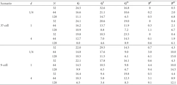
We further extend this example by varying𝑁 ∈ {32, 64, 128}
and the parameter 𝑑 ∈ {1/4, 1, 4} and simulate the same
scenario. Let G, GI, and GO denote the empirical expected
values of the quantities 𝐺, 𝐺𝐼𝑖,𝑗, and 𝐺𝑂𝑖,𝑗, respectively, out
of the 400 simulation instances. Also, let P, PI, and PO
Table 4: The comparative results associated with OFFR and BFFR when the system parameters𝑑 and 𝑁 are varied. Scenario 𝑑 𝑁 G GI GO PI PO 32 24.5 32.6 16.8 0 0.5 1/4 64 16.6 21.1 10.6 0.2 2.0 128 11.1 14.7 6.5 0.5 6.8 32 24.1 20.6 19.0 0 0.4 37-cell 1 64 16.2 13.7 11.9 0.3 2.1 128 10.9 8.8 7.2 1.1 6.7 32 19.8 10.5 23.5 0 0.4 4 64 12.7 7.0 14.5 0.1 1.9 128 8.0 4.6 8.9 0.6 6.1 32 22.0 29.5 14.5 0.7 4.3 1/4 64 14.8 17.6 9.0 3.0 10.0 128 10.5 11.5 6.1 6.1 15.0 32 22.1 17.8 16.1 0.6 4.3 9-cell 1 64 14.5 10.5 9.8 4.4 10.0 128 9.9 6.5 6.7 9.4 14.5 32 16.4 9.4 19.8 0.5 4.4 4 64 10.3 5.8 12.3 3.1 8.9 128 6.5 3.4 8.3 9.1 12.1
respectively, which are below zero, that is, those scenarios or users who do not benefit from OFFR. Table 4 provides the
quantities G, GI, GO, PI, and PO, for varying choices of𝑑
and𝑁. We note that the quantity P is found to be zero for
all studied cases; that is, all networks benefited from OFFR in comparison with BFFR in terms of average throughput. Our further findings are as follows:
(i) As the number of users in the network increases, the average gain obtained with OFFR decreases and moreover the fraction of users that do not benefit
from OFFR also increases with increased 𝑁. The
OFFR gain becomes more substantial when the num-ber of users in the network is relatively smaller. This observation can be explained by the fact that when there is just one user or few users within a cell (which happens when the overall number of users is small), opportunistic scheduling within a cell as in BFFR is not as effective. In such scenarios, network-wide opportunistic scheduling helps the network users significantly.
(ii) The OFFR average gains are slightly more substantial in the 37-cell network than the 9-cell network. (iii) Only a relatively small fraction of users appeared to
fail to gain with OFFR. This quantity is observed to diminish significantly in the particular 37-cell network scenario. For example, in the worst case, for the 37-cell network scenario, only 6.8% (1.1%) of the
outer (inner) users failed to gain with OFFR for𝑑 =
1/4 (𝑑 = 1) out of all the studies we have performed.
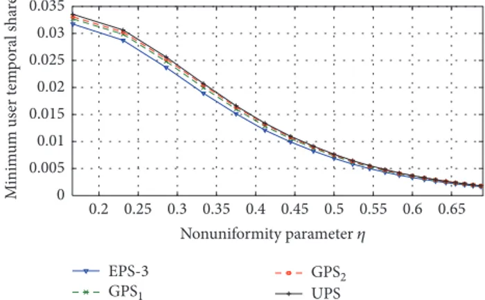
4.3. Impact of GPS Selection for the MMTF Formulation.
In this section, we study the impact of the choice of the underlying pattern set in the context of MMTF problem
(10). The performance metric is taken as the minimum of the temporal shares of all the users served in the CN (𝑧 in (10)). Recall that MMTF attempts to maximize this quantity through the linear program given in Section 3.2 through which we obtain the per-pattern weights for this numerical example and consequently the performance metric. For this
purpose, given the CNs with𝐾 = 6 or 9 cells depicted in
Figure 5,10𝐾 users are spread through the CN uniformly,
leading to an average population of 10 users per cell. After
locating 10𝐾 users in the CN, one section is selected at
random and 10𝑃, 𝑃 ∈ {1, 2, . . . , 10} users are further
introduced in this cell for the purpose of making the user distribution through the network more nonuniform. To
quantify this nonuniformity, we introduce the parameter𝜂 =
(1 + 𝑃)/(𝐾 + 𝑃) which gives the expected number of users in the most crowded cell divided by the overall number of users
in the network. The larger the parameter𝑃 or 𝜂 is, the more
nonuniform the user distribution becomes. Subsequently, each MMTF problem is solved 1000 times each of which is
obtained by associating10(𝐾 + 𝑃) users in the CN with the
individual cells and their sections. The average of the 1000 instances is then reported. We first study the 9-cell scenario given in Figure 5(a). We study the following pattern sets in the simulation study (the individual patterns are defined in Table 1):
(i) GPS1={𝑃1, 𝑃2, 𝑃3, 𝑃4, 𝑃5, 𝑃8, 𝑃11, 𝑃15, 𝑃22, 𝑃29}
(ii) GPS2= GPS1∪ {𝑃24, 𝑃36}
(iii) GPS3= GPS2∪ {𝑃6, 𝑃10, 𝑃17, 𝑃19, 𝑃21}
(iv) GPS4: pattern set obtained by Algorithm 1 with
cardinality 22 which is presented in Table 1 (v) EPS-3