Selçuk J. Appl. Math. Selçuk Journal of Vol. 13. No. 2. pp. 43-62, 2012 Applied Mathematics
Di¤erent Linearization Techniques for the Numerical Solution of the MEW Equation
S. Battal Gazi Karakoc1, Yusuf Ucar2, N. Murat Yagmurlu3
1Department of Mathematics, Faculty of Science and Art, Nevsehir University,
Nevse-hir, 50300, Turkiye
e-mail:sbgkarako c@ nevsehir.edu.tr
2Department of Mathematics, Faculty of Science and Art, Inonu University, Malatya,
44280, Turkiye
e-mail:yusuf.ucar@ inonu.edu.tr
3Department of Mathematics, Faculty of Science and Art, Inonu University, Malatya,
44280, Turkiye
e-mail:murat.yagmurlu@ inonu.edu.tr
Received Date: April 30, 2012 Accepted Date: December 1, 2012
Abstract. The modi…ed equal width wave (MEW) equation is solved numeri-cally by giving two di¤erent linearization techniques based on collocation …nite element method in which cubic B-splines are used as approximate functions. To support our work three test problems; namely, the motion of a single solitary wave, interaction of two solitary waves and the birth of solitons are studied. Results are compared with other published numerical solutions available in the literature. Accuracy of the proposed method is discussed by computing the nu-merical conserved laws L2and L1error norms. A linear stability analysis of the approximation obtained by the scheme shows that the method is unconditionally stable.
Key words: Finite element method; Collocation; MEW equation; B-Spline; Solitary waves.
2000 Mathematics Subject Classi…cation: 97N40, 65N30, 65D07, 76B25, 74S05, 74J35.
1. Introduction
This paper is concerned with applying the cubic B-spline function to develop a numerical method for approximating the analytic solution of the MEW equation which was introduced by Morrison et al.[9] as a model for nonlinear dispersive
waves. This equation has been solved analytically for a limited set of boundary and initial conditions. So the numerical solutions of the MEW equation have been the subject of many studies [1-7,11-19]. In this paper, we have used two di¤erent linearization techniques to obtain the numerical solution of the MEW equation. The performance of the method has been tested on three numerical wave propagation experiments: the motion of a single solitary wave, the inter-action of two solitary waves and birth of solitons. The stability analysis of the the approximation obtained by the method is also investigated.
2. The Governing Equation and Collocation Solutions MEW equation takes the form of
(1) Ut+ 3U2Ux Uxxt= 0; a x b
with the physical boundary conditions U ! 0 as x ! 1; where t is time , x is the space coordinate and is a positive parameter. Appropriate boundary conditions will be chosen as
(2) U (a; t) = 0; U (b; t) = 0;
Ux(a; t) = 0; Ux(b; t) = 0:
Let us consider the interval [a; b] is partitioned into N …nite elements of uni-formly equal length by the knots xi, i = 0; 1; 2; :::; N such that a = x0 < x1 < xN = b and h = (xi+1 xi). The cubic B-splines i(x) , (i = -1(1) N+1), at the knots xi are de…ned over the interval [a; b] by [8] (3) i(x) =h13 8 > > > > < > > > > : (x xi 2)3; x 2 [xi 2; xi 1]; h3+3h2(x x i 1) + 3h(x xi 1) 2 3(x xi 1)3; x 2 [xi 1; xi]; h3+3h2(x i+1 x) + 3h(xi+1 x) 2 3(xi+1 x)3; x 2 [xi; xi+1];
(xi+2 x)3; x 2 [xi+1; xi+2];
0 otherwise:
The set of splines 1(x); 0(x); : : : ; N +1(x) forms a basis for the functions de…ned over [a,b]. Therefore, an approximation solution UN(x; t) can be written in terms of the cubic B- splines as trial functions:
(4) UN(x; t) =
N +1X i= 1
i(x) i(t)
where i’s are unknown, time dependent quantities to be determined from the boundary and cubic B-spline collocation conditions. Each cubic B-spline covers four elements so that each element [xi; xi+1] is covered by four cubic B-splines. For this problem, the …nite elements are identi…ed with the interval [xi; xi+1]
and the elements knots xi; xi+1. Using the nodal values Ui; U
0
i and U
00
i are given in terms of the parameter i by:
(5) Ui= U (xi) = i 1+ 4 i+ i+1; U0 i = U0(xi) = 3h( i 1+ i+1); U00 i = U00(xi) = h62( i 1 2 i+ i+1)
and the variation of UN(x; t) over the typical element [xi; xi+1] is given by
(6) UN(x; t)=
i+2 X j=i 1
j(t) j(x) :
If we substitute the global approximation (4) and its necessary derivatives (5) into Eq. (1), we obtain the following set of the …rst order ordinary di¤erantial equations: (7) _i 1+ 4 _i+ _i+1+ 9Zi 2h( i 1+ i+1) 6h2( _i 1 2 _i+ _i+1) = 0 where Zi = ( i 1+ 4 i+ i+1)2
and : denotes derivative with respect to time. If time parameters
i’s and its time derivatives _i’s in Eq. (7) are discretized by the Crank-Nicolson formula and usual …nite di¤erence aproximation, respectively:
(8) i= 1 2( n + n+1); _i= n+1 n t
we obtain a recurrence relationship between two time levels n and n + 1 relating two unknown parameters n+1i ; ni for i = m 1; m; m + 1;
(9) m1 n+1m 1+ m2 n+1 m + m3 n+1 m+1= m3 n m 1+ m2 n m+ m1 n m+1 where (10) m1= (1 EZm ); m2= (4 + 2M ); m3= (1 + EZm M ) m = 0; 1; : : : ; N; E =2h9 t; M = h62 :
For the …rst linearization (First Lin.), we suppose that the quantity U in the non-linear term U2U
x to be locally constant. This is equivalent to assuming that in Eq. (7) all U ’s are equal to a local constant Zi:
For the second linearization (Second Lin.), using …rst order di¤erence formula for the time derivative of the U and Crank-Nicolson approximation for the space derivatives Ux and Uxxin Eq. (1) lead to
(11) U n+1 Un t + 3 (U2Ux)n+1+ (U2Ux)n 2 Uxxn+1 Uxxn t = 0:
Now, if we apply Rubin and Graves [17] linearization technique to Eq. (11) (U2Ux)n+1= Un+1UnUxn+ UnUn+1Uxn+ UnUnUxn+1 2U UnUxn we obtain (12) U n+1+ 3 t 2 (U n+1UnUn x + UnUn+1Uxn+ UnUnUxn+1) Uxxn+1 = Un 3 t 2 (U2Ux)n Uxxn + 6 2t(UnUnUxn): The system (9) consists of N + 1 linear equations including N + 3 unknown pa-rameters ( 1; : : : ; N +1)T. To obtain a unique solution to this system, we need two additional constraints. These are obtained from the boundary conditions and can be used to eliminate 1 and N +1 from the system (9) which then becomes a matrix equation for the N + 1 unknowns d = ( 0; 1; : : : ; N)T of the form
(13) Adn+1= Bdn:
The matrices A and B are tridiagonal (N + 1) (N + 1) matrices and so are easily solved . However, two or three inner iterations are applied to the term
n
= n+12( n n 1) at each time step to cope with the non-linearity caused by Zi.
2.1. Initial state
The initial vector d0 is determined from the initial and boundary conditions. So the approximation (4) must be rewritten for the initial condition
(14) UN(x; 0)=
N +1X i= 1
0
i(t) i(x)
where the 0i’s are unknown parameters. We require the initial numerical ap-proximation UN(x; 0) satisfy the following conditions:
(15) UN(x; 0) = U (xi; 0); i = 0; 1; :::; N (UN)x(a; 0) = 0; (UN)x(b; 0) = 0: Thus, these conditions lead to matrix equation
(16) W d0= b where W = 2 6 6 6 6 6 6 6 4 4 2 1 4 1 1 4 1 . .. 1 4 1 2 4 3 7 7 7 7 7 7 7 5
d0= ( 0; 1; 2; : : : ; N 2; N 1; N)T
and
b = (U (x0; 0); U (x1; 0); U (x2; 0); : : : ; U (xN 2; 0); U (xN 1; 0); U (xN; 0))T:
2.2. Stability analysis
The investigation of the stability of the approximation obtained by the algorithm will be based on the von Neumann theory in which the growth factor of a typical Fourier mode is de…ned as:
(17) nj = ^neijkh;
where k is the mode number and h is the element size. Thus the stability analysis is determined for the linearisation of the approximation obtained by the numer-ical scheme. Substituting the Fourier mode (17) into the linearised recurrence relationship (9) shows that the growth factor for mod k is
(18) g = a ib
a + ib where
(19) a = 2 + M + (1 M ) cos[hk];
b = EZisin[hk]:
The modulus of jgj is 1, therefore the linearised scheme is unconditionally stable. 3. Numerical Examples and Results
Numerical results of the equation for the three test problems were obtained and all computations were executed on a pentium PC4 in the Fortran code using double precision arithmetic. The MEW Eq. (1) possesses only three following conservation laws: (20) I1= Rb a U dx ' h PN J =1Ujn; I2=RabU2+ (Ux)2dx ' hPNJ =1(Ujn)2+ (Ux)nj; I3= Rb a U 4dx ' hPN J =1(Ujn)4:
which correspond to mass, momentum and energy respectively [10]. The accu-racy of the method is measured by both the error norm L2
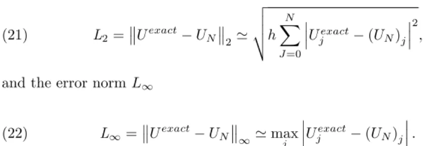
(21) L2= Uexact UN 2' v u u thXN J =0 Uexact j (UN)j 2 ;
and the error norm L1
(22) L1= Uexact UN 1' max
j U
exact
j (UN)j :
To implement the method, three test problems: motion of a single solitary wave, interaction of two solitary waves and the maxwellian initial condition will be considered.
4. Motion of a Single Solitary Wave
The solitary wave solution of the MEW Eq.(1) is given by U (x; t) = A sec h(k[x x0 vt])
where k =p1= , v = A2=2. This solution corresponds to motion of a single solitary wave of magnitude A; initially centered at the position x0 and propa-gating to the right side with a constant velocity v. The initial condition is
U (x; 0) = A sec h(k[x x0]):
For this problem the analytical values of the invariants are [14]
(23) I1= A k ; I2= 2A2 k + 2 kA2 3 ; I3= 4A4 3k :
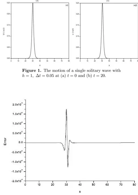
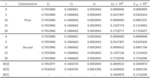
The analytical values of the invariants are obtained from Eq. (1) as I1 = 0:7853982 , I2 = 0:1666667 , I3= 0:0052083. To compare our results with the earlier papers, parameters are taken as t = 0:05; = 1; x0 = 30; A = 0:25 and the interval 0 x 80 is divided into elements of equal lenght h = 0:1. The simulation is run up to time t = 20, and the three invariants I1; I2 and I3 and error norms L2, L1are listed for the duration of the simulation. In Table 1, we compare the values of the invariants and error norms obtained using the present method with di¤erent approximations and those of [2, 5, 7] at di¤erent times. As seen from the table, the error norms L2and L1are found to be small enough and the quantities in the variants remain almost constant during the computer run. While for the …rst linearization, invariants I1; I2and I3change by less than 0:03 10 5%, 5:48 10 5%, 0:33 10 5% for the second linearization they change less than 0:02 10 5%, 5:50 10 5%, 0:30 10 5% throught the run, respectively. Thus it is seen that the invariants remain satisfactorily constant. Figure 1 shows that the proposed method performs the motion of propagation
of a solitary wave satisfactorily, which moves to the right at a constant speed and preserves its amplitude and shape with increasing time as expected. The amplitude is 0:25 at t = 0 and located at x = 30:6, while it is 0:249880 at t = 20 and located at x = 30:6. The absolute di¤erence in amplitudes at times t = 0 and t = 20 is 12 10 5so that there is a little change between amplitudes. The error graph at t = 20 is given in Figure 2. As it is seen, the maximum errors occur around the central position of the solitary wave.
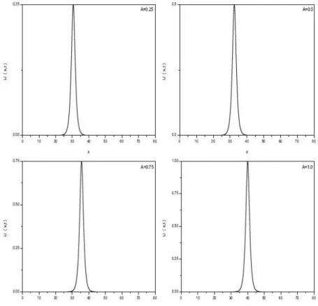
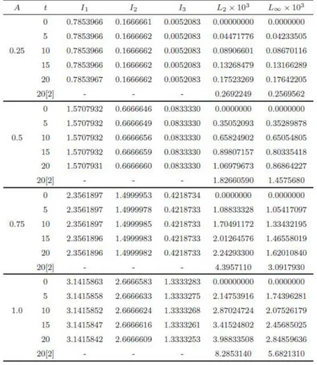
This problem is also considered for di¤erent values of the amplitude at h = 0:1 and t = 0:01. In Table 2, the error norms and the invariants are listed for A = 0:25; 0:5; 0:75; 1: A comparison with Ref. [2] shows that the present method provides better results in terms of the error norms L2and L1. Figure 3 shows the solutions of the single solitary wave with h = 0:1; t = 0:01 for di¤erent values of amplitude A at time t = 20: It is clear that the soliton moves to the right at a constant speed and almost preserves its amplitude and shape with increasing of time, as expected.
5. Interaction of Two Solitary Waves
Now we consider Eq. (1) together with boundary conditions U ! 0 as x ! 1 and the initial condition for all linearization techniques as
U (x; 0) = 2 X j=1 Ajsec h(k[x xj]) where k =p1= .
Firstly, we have studied the interaction of two positive solitary waves with the parameters h = 0:1; t = 0:025; = 1; A1 = 1; A2 = 0:5 ; x1= 15; x2 = 30 through the interval 0 x 80: The analytical values can be found as follows [5]:
(24)
I1= (A1+ A2) = 4:7123889; I2=83(A21+ A22) = 3:3333333; I3=43(A41+ A42) = 1:4166667:
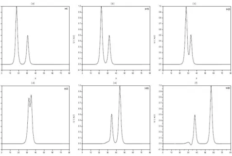
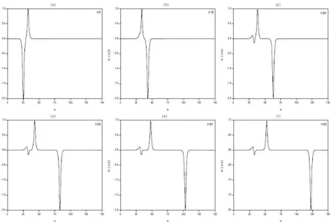
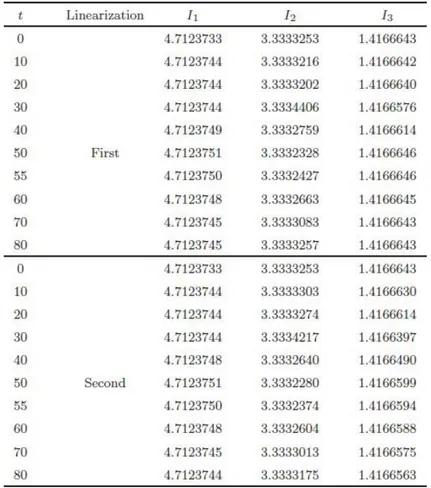
The experiment was run from time t = 0 to time t = 80 to allow the interaction take place. In Figure 4, we show the interaction of two positive solitary waves at di¤erent times. It can be seen that at time t = 5 the wave with larger amplitude is to the left of the second wave with smaller amplitude. The larger wave catches up the smaller one as time increases. Interaction starts at about time t = 25, overlapping processes occurres between times t = 25 and t = 40 and the waves start to resume their original shapes after time t = 40. An oscillation of small amplitude trailing behind the solitary waves in Fig. 4(f) was observed. In order to see this oscillation the scale of Fig. 4(f) was magni…ed as shown in Fig 5. At time t = 80; for the …rst linearization the amplitude of the larger wave is 0:999694 at the point x = 44:4 whereas the amplitude of
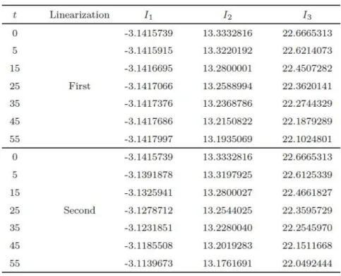
the smaller one is 0:510405 at the point x = 34:7. For the second linearization, the amplitude of the larger wave is 0:999716 at the point x = 56:9 whereas the amplitude of the smaller one is 0:498438 at the point x = 37:7. Table 3 compares the values of the invariants of the two solitary waves with the obtained results from the …rst and the second linearization. The absolute di¤erence between the values of the invariants obtained by the …rst linearization at times t = 0 and t = 80 are I1 = 1:2 10 6; I2 = 4 10 7; I3 = 0 whereas they are I1= 1:1 10 6; I2= 7:8 10 6; I3= 8 10 66 for the second linearization. Secondly, for the solitary of amplitudes 2 and 1 to interact, we have chosen the region as 0 x 150 while keeping all other parameters the same as given before. The experiment was run from time t = 0 to time t = 55 to allow the interaction take place. Figure 6 shows the development of the solitary wave interaction. As it is seen from the Figure 6, at t = 0 a wave with the negative amplitude is to the left of another wave with the positive amplitude. The larger wave with the negative amplitude catches up the smaller one with the positive amplitude as time increases. At t = 55, for the …rst linearization the amplitude of the smaller wave is 0:974353 at the point x = 52:5, whereas the amplitude of the larger one is 1:986150 at the point x = 122:7. It is found that the absolute di¤erence in amplitudes is 0:256 10 1 for the smaller wave and 0:138 10 1for the larger one. For the second linearization, the amplitude of the smaller wave is 0:973607 at the point x = 52:5, whereas the amplitude of the larger one is 1:988065 at the point x = 123:6. It is found that the absolute di¤erence in amplitudes is 0:263 10 1 for the smaller wave and 0:119 10 1 for the larger one. The analytical invariants by using Eq.(1) can be found as I1= 3:1415927, I2= 13:3333333, I3= 22:6666667. Table 4 lists the values of the invariants of the two solitary waves with amplitude A1 = 2 and A2 = 1 in the region 0 x 150 . It can be seen that the values obtained for the invariants are satisfactorily constant during the computer run.
5.1. The Maxwellian initial condition
For this equation another initial value problem is the initial Maxwellian pulse that is used as the initial condition in solitary waves given by
(25) U (x; 0) = e x2
with the boundary condition
U ( 20; t) = Ux( 20; t) = U (20; t) = Ux(20; t) = 0; t > 0:
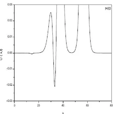
As it is known Maxwellian initial condition (25) breaks up into a number of solitary waves depending on values of : So we have used various values for : During the run of algorithms, we have taken h = 0:1; t = 0:01: The com-putations are carried out for the cases of = 1; 0:5; 0:1; 0:05; 0:02 and 0:005 . For = 1; the Maxwellian initial condition develops into a pair of waves as indicated in Figure 7. One wave with the negative amplitude is to the left of the other wave with the positive amplitude. For = 0:5; the Maxwellian initial
condition does not cause development into a clean solitary wave. When = 0:1; we observed one clean solitary wave. For = 0:05; the state is two solitary waves. For = 0:02 and 0:005 three and seven solitary waves are formed, respectively. The recorded values of the invariants I1; I2 and I3 computed for both linerazation techniques are given in Table 5 and 6. It is observed that the obtained values of the invariants remain almost constant during the computer run.
6. Conclusions
In this paper, numerical solutions of the MEW equation based on the cubic B-spline …nite element have been presented. Three test problems are worked out to examine the performance of the algorithms. The performance and accuracy of the method is shown by calculating the error norms L2 and L1. For each linearization technique, the error norms are su¢ ciently small and the invariants are satisfactorily constant in all computer runs. The computed results show that the present method is a remarkably successful numerical technique for solving the MEW equation and advisable for getting numerical solutions of other types of non-linear equations.
References
1. A. Esen, A lumped Galerkin method for the numerical solution of the modi…ed equal width wave equation using quadratic B splines, International Journal of Computer Mathematics,Vol.83, Nos, 5-2 May-June 2006, pp. 449-459.
2. A. Esen and S. Kutluay, Solitary wave solutions of the modi…ed equal width wave equation, Communications in Nonlinear Science and Numerical Simulation 13(2008) 1538-1546.
3. A. M. Wazwaz, The tanh and sine-cosine methods for a reliable treatment of the modi…ed equal width equation and its variants, Communications in Nonlinear Science and Numerical Simulation, 11, 148-160 (2006).
4. B. Saka, Algorithms for numerical solution of the modi…ed equal width wave equa-tion using collocaequa-tion method , Mathematical and Computer Modelling, 45 (2007) 1096-1117.
5. D. J. Evans and K. R. Raslan, Solitary waves for the generalized equal width (GEW) equation, Int.J.Comput.Math.82(4) (2005) 445-455.
6. J. Lu , He’s variational method for the modi…ed equal width wave equation, Chaos solitons and Fractals (2007).
7. K. R. Raslan, Collocation method using cubic B-spline for the generalized equal width equation, Int. J. Simulation and Process Modelling, Vol. 2, Nos.1/2, 2006. 8. P. M. Prenter, Splines and Variasyonel Methods, 1975,(New York:John Wiley) 9. P. J. Morrison, J. D. Meiss and J. R. Carey Scattering of RLW solitary waves, Physica 11 D 324-336 (1984).
10. P. J. Olver, Euler operators and conservation laws of the BBM equations, Math. Proc. Camb. Phil. Soc. 85: 143-159, 1979.
11. S. Hamdi, W. E. Enright, W. E .Schiesser, J. J. Gottlieb and Abd Alaal, Exact solutions of the generalized equal width wave equation, in: Proceedings of the Interna-tional Conference on ComputaInterna-tional Science and Its Application, in: LNCS, vol.2668, Springer-Verlog, 2003, pp.725-734.
12. Seydi Battal Gazi Karakoç, Numerical solutions of the modi…ed equal width wave equation with …nite elements method, Ph.D. Thesis, Inonu University, December 2011. 13. S. Battal Gazi Karakoç and T. Geyikli , Numerical Solution of the modi…ed equal width wave equation , International journal of di¤erential equations, Vol. 2012, ID. 587208, doi:10.1155, 15 pages, 2012.
14. S. I. Zaki, Solitary wave interactions for the modi…ed eual width equation, Comput. Phys. Com. 126 , 219-231,(2000).
15. S. Islam, F. Haq and I. A. Tirmizi, Collocation method using quartic B-spline for numerical solution of the modi…ed equal width wave equation, Journal of Applied Mathematics and Informatics, Vol.28, No.3-4, (2010), 611-624.
16. S. T. Mohyud-Din, A. Y¬ld¬r¬m, M. E. Berberler and M. M. Hosseini, Numerical solution of the modi…ed equal width wave equation, World Applied Science Journal, Vol.8, No.7, (2010), 792-798.
17. Stanley G. Rubin and Randolph A. Graves, A Cubic spline approximation for problems in ‡uid mechanics, Nasa TR R-436, Washington, DC, 1975.
18. T. Geyikli and S. Battal Gazi Karakoç, Septic B-Spline collocation method for the Numerical Solution of the modi…ed equal width wave equation , Applied mathematics, Vol. 2, No. 6, (2011), 739-749.
19. T. Geyikli and S. Battal Gazi Karakoç, Petrov-Galerkin method with cubic B-splines for solving the MEW equation, Bulletin of the Belgian Mathematical Society, (Accepted for publication).
Figures and Tables
Figure 1. The motion of a single solitary wave with h = 1; t = 0:05 at (a) t = 0 and (b) t = 20.
Figure 3. Single solitary wave solutions for various values of A at t = 20:
Figure 6. Interaction of two solitary waves at di¤erent times.
Figure 7. Maxwellianinitialcondition,stateattime t = 12; a) = 1; b) = 0:5; c) = 0:1; d) = 0:05; e) = 0:02; f ) = 0:005
Table 1. The invariants and the error norms for single solitary wave with h = 0:1; t = 0:05; A = 0:25; 0 x 80:
Table 2. The computed values I1; I2 and I3 and the error norms L2 and L1for the single solitary wave with x0= 30; h = 0:1; t = 0:01 in the region 0 x 80:
Table 3. Invariants and error norms for single solitary wave with A1= 1; A2= 0:5; h = 0:1; t = 0:05
Table 4. Invariants and error norms for single solitary wave with A1= 2; A2= 1; h = 0:1; t = 0:05
Table 5. The invariants I1; I2and I3 obtained during the …rst linerazation technique for Maxwellian initial condition and di¤erent values of :
Table 6. The invariants I1; I2and I3 obtained during the second linerazation technique for Maxwellian initial condition and di¤erent values of :