Synthesis of lossless ladder networks with simple lumped elements connected via commensurate transmission lines

Received on: 28.10.2010 Accepted on: 21.12.2010

SYNTHESIS OF LOSSLESS LADDER

NETWORKSWITH SIMPLE LUMPED ELEMENTS

CONNECTED VIACOMMENSURATE TRANSMISSION LINES

Metin ŞENGÜL

Kadir Has University, Engineering Faculty, Cibali-Fatih,Istanbul, Turkey

msengul@khas.edu.tr

Abstract: An algorithm has been proposed, to synthesize low-pass, high-pass, band-pass and band-stop lossless ladder networks with simple lumped elements connected via commensurate transmission lines (Unit elements, UEs). First, the type of the element that will be extracted is determined from the given mixed-element network function. After obtaining element value, it is extracted, and the two-variable reflection function of the remaining mixed-element network is obtained. This process is repeated until extracting all the elements. For each network type, an example is included, to illustrate the implementation of the related algorithm.

Keywords: Synthesis, Mixed lumped and distributed elements, Ladder networks, Scattering matrix.

1. Introduction

The design problem with mixed lumped and distributed elements requires the characterization of the mixed-element structures using transcendental or multivariable functions. The first approach deals with non-rational single variable transcendental functions and is based on the study of cascaded non-commensurate transmission lines by Kinarivala [1]. First results on the synthesis of a transcendental driving-point impedance function as a cascade of lumped, lossless, two-ports and commensurate transmission lines were given by Riederer and Weinberg [2]. The other approach to describe mixed lumped and distributed two-ports is based on Richards transformation, tanh(p) which converts the transcendental functions of a distributed network into rational functions [3]. The attempts to generalize this approach to mixed lumped and distributed networks led to the multivariable synthesis procedures, where the Richards variable  is used for distributed-elements and the original frequency variable p for lumped-elements. In this way, all the network functions could be written as rational functions of two complex variables. After the work of Ozaki and Kasami [4] on the multivariable positive real functions, the network design problem with mixed lumped and distributed elements is attempted to be solved by many researchers especially using the multivariable approach. In this context, although there have been valuable contributions, a complete theory for the approximation and synthesis problems of mixed lumped and distributed networks is still not available.

At the end of a circuit design process, after getting the network function which meets the design specifications, it is necessary to obtain the circuit structure and element values. So here, a synthesis

algorithm has been proposed to extract the element values from the given two-variable network function of a special type structure called lossless ladder networks with simple lumped elements connected via commensurate transmission line.

In the following section, the characterization of two-variable networks is introduced. Subsequently, after giving the synthesis algorithm, examples are presented, to illustrate the utilization of the proposed algorithm.

2. Characterization of Two-variable Networks

Figure 1. Lossless two-port with input reflectance function ) , ( 11 p S .

Let



Skl;k,l1,2



designate the scattering parameters of a lossless two-port like the one depicted in figure 1. For a mixed lumped and distributed element, reciprocal, lossless two-port, the scattering parameters may be expressed in Belevitch form as follows [5-8].

                   ) , ( ) , ( ) , ( ) , ( ) , ( 1 ) , ( ) , ( ) , ( ) , ( ) , ( 22 21 12 11             p h p f p f p h p g p S p S p S p S p S (1) where ) , ( ) , (    p f p f    .

In (1), pj is the usual complex frequency variable associated with lumped-elements, and j

is the Richards variable associated with equal-length transmission lines or so called commensurate transmission

lines (tanhp, where  is the commensurate delay of the distributed elements).

) , (p

g is (npn)th degree scattering Hurwitz

polynomial with real coefficients such that P λ λ PT g T Tg p g( ,)    , where                   n n n n g p p g g g g g g g          0 11 10 0 01 00 ,



1



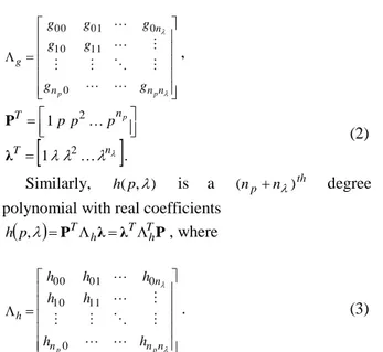
. 1 2 2     n T n T p p p p         λ P (2) Similarly, h(p,) is a (npn)th degree

polynomial with real coefficients

 

p PT hλ λT ThP h ,     , where                   n n n n h p p h h h h h h h          0 11 10 0 01 00 . (3) ) , (p

f is a real polynomial which includes all the transmission zeros of the two-port network.

Since the network is considered as a lossless two-port terminated in a resistance, then energy conversation requires that

I p S p

S( ,) T( ,) , (4) where I is the identity matrix. The open form of (4) is given as ). , ( ) , ( ) , ( ) , ( ) , ( ) , (pgp h php f p f p g (5)

The fundamental properties of this kind of mixed-element structures can be found in [6, 9-10]. In the following section, the proposed synthesis algorithm is given.

3. Algorithm

In the flowchart seen in figure 2, the proposed synthesis algorithm has been given. Shortly, after calculating the constants (₁ and ₂ 1) from the given two-variable reflection function, the types of the first and the second components are decided. Then the value of the first element and the reflection function of the remaining network are calculated. After extracting the second component, it is not necessary to decide the type of the next element, since the network has a ladder structure. After calculating all the element values, the algorithm is stopped.

Figure 2. Flowchart of the proposed synthesis algorithm.

In the following part, synthesis algorithm has been detailed for low-pass, high-pass, band-pass and band-stop mixed-element structures.

3.1. Low-pass Ladders Connected with Unit

Elements

The coefficient matrices of the polynomials h(p,) and )

, (p

g , and polynomial f(p,) describing the mixed-element low-pass structure are as follows,

, 0 0 0 0 0 0 21 20 1 12 11 10 0 02 01 00                            p n n n h h h h h h h h h h h h   , 0 0 0 0 0 0 21 20 1 12 11 10 0 02 01 00                            p n n n g g g g g g g g g g g g   . ) 1 ( ) , (p  2 n/2 f   Step 1: 1 1  2 1 If 0 ) 1 , ( 0 ) 1 , (   p p n g n h If 0 ) 1 , ( 0 ) 1 , (   p p n g n h ) 0 , ( ) 0 , ( p p n g n h ) 1 , ( ) 1 , ( p p n g n h ) 1 , 1 ( ) 1 , 1 (   p p n g n h Step 2: 1

 2 First component Next component

+1 -1 UE Series inductor (L) -1 +1 UE Parallel capacitor (C) h  ,_g,f :Given Calculate 1  , 2

Decide the first and the second element types

Calculate the element value Extract the element,

calculate h, g and f of the remaining network Stop Y All elements extracted ? N Start

+1 +1 Series inductor (L) UE -1 -1 Parallel capacitor (C) UE

Step 3: Element

Type Unit Element Series Inductor Parallel Capacitor

Element Value ) ( 11 ) ( 11 1 1   S S Z    where





      n i n i i g i h S 0 0 ) ( 11 ) , 0 ( ) , 0 ( ) 0 , 1 ( ) 0 , 1 ( ) 0 , ( ) 0 , ( 1 1      p p p p n h n g n h n g L   ) 0 , 1 ( ) 0 , 1 ( ) 0 , ( ) 0 , ( 1 1      p p p p n h n g n h n g C   Polynomial g of the extracted element 1 2 1 2   _ Z Z 1 2 p L 1 2 p C Polynomial h of the extracted element  Z Z 2 1 2_ p L 2 p C 2  Polynomial f of the extracted element 2 / 1 2 ) 1 (  1 1 Polynomial ) , ( ) ( _ p g RN of the remaining network ) , ( ) ( ) , ( ) (     p g g p h h     h(p)h(p,)g(p)g(p,) ) , ( ) ( ) , ( ) ( ph p g p g p h    Polynomial ) , ( ) ( _ p h RN of the remaining network ) , ( ) ( ) , ( ) (     p g h p h g  g(p)h(p,)h(p)g(p,) g(p)h(p,)h(p)g(p,) Polynomial ) , ( ) ( _ p f RN of the remaining network 2 / ) 1 ( 2 ) 1 (  n 2 /2 ) 1 ( _ n

Step 4: Set new h(p,),g(p,) and f(p,) two-variable polynomials as h(p,)h(RN)(p,), ) , ( ) , (p g( ) p  g  RN , f(p,) f(RN)(p,), and go to Step 3.

3.2. High-Pass Ladders Connected with Unit Elements

The polynomial f(p,) and the coefficient matrices of the polynomials h(p,) and g(p,) describing the mixed-element high-pass structure are as follows,

2 / 2 ) 1 ( ) , (  n_p  n p p f   , _, 0 0 2 1 0 1 12 11 2 21 20 12 10 01 00                           n n n n n n n n n n n n h p p p p p p p p p h h h h h h h h h h h h h h          . 0 0 2 1 0 1 12 11 2 21 20 12 10 01 00                           n n n n n n n n n n n n g p p p p p p p p p g g g g g g g g g g g g g g         

Step 1: 1 1  2 1 If 0 ) 1 , 0 ( 0 ) 1 , 0 (   g h If 0 ) 1 , 0 ( 0 ) 1 , 0 (   g h ) 0 , 0 ( ) 0 , 0 ( g h ) 1 , 0 ( ) 1 , 0 ( g h ) 1 , 1 ( ) 1 , 1 ( g h Step 2: 1

 ₂ First component Next component

+1 -1 UE Series capacitor (C) -1 +1 UE Parallel inductor (L) +1 +1 Series capacitor (C) UE -1 -1 Parallel inductor (L) UE Step 3: Element

Type Unit Element Parallel Inductor Series Capacitor

Element Value ) ( 11 ) ( 11 1 1   S S Z    where





      n i p n i p i n g i n h S 0 0 ) ( 11 ) , ( ) , ( ) 0 , 0 ( ) 0 , 0 ( ) 0 , 1 ( ) 0 , 1 ( 1 1 h g h g L      ) 0 , 0 ( ) 0 , 0 ( ) 0 , 1 ( ) 0 , 1 ( 1 1 h g h g C      Polynomial g of the extracted element 1 2 1 2   _ Z Z L p 2 1  C p 2 1  Polynomial h of the extracted element  Z Z 2 1 2_ L 2 1  C 2 1 Polynomial f of the extracted element 2 / 1 2 ) 1 (  p p Polynomial ) , ( ) ( _ p g RN of the remaining network ) , ( ) ( ) , ( ) (     p g g p h h     ) , ( ) ( ) , ( ) ( ph p g p g p h   h(p)h(p,)g(p)g(p,) Polynomial ) , ( ) ( _ p hRN of the remaining network ) , ( ) ( ) , ( ) (     p g h p h g  g(p)h(p,)h(p)g(p,) g(p)h(p,)h(p)g(p,) Polynomial ) , ( ) ( _ p f RN of the remaining network 2 / ) 1 ( 2 ) 1 (  n 1 2 /2 ) 1 (  n n_p p  

Step 4: Set new h(p,),g(p,) and f(p,) two-variable polynomials as h(p,)h(RN)(p,), ) , ( ) , (p g( ) p g  RN , f(p,) f(RN)(p,), and go to Step 3.

3.3. Band-Pass Ladders Connected with Unit Elements

The polynomial f(p,) and the coefficient matrices of the polynomials

) , (p

h and g(p,) describing the mixed-element band-pass structure are as follows,

2 / 2 2 / ) 1 ( ) , (  n_p  n p p f   , , 0 0 0 0 0 0 0 0 0 0 0 0 0 0 0 11 10 2 2 2 1 2 0 2 11 10 00                                        p p p p p p p n n n n n n n n h h h h h h h h h h h                                0 0 0 0 0 0 0 0 0 0 0 0 0 0 0 11 10 2 2 2 1 2 0 2 11 10 00            p p p p p p p n n n n n n n n g g g g g g g g g g g  Step 1: 1 1  ₂1 If 0 ) 1 , 0 ( 0 ) 1 , 0 (   g h If 0 ) 1 , 0 ( 0 ) 1 , 0 (   g h If 0 ) 1 , 1 ( 0 ) 1 , 1 (   g h If 0 ) 1 , ( 0 ) 1 , (   p p n g n h ) 0 , 0 ( ) 0 , 0 ( g h ) 1 , 0 ( ) 1 , 0 ( g h ) 1 , 1 ( ) 1 , 1 ( g h ) 1 , ( ) 1 , ( p p n g n h ) 1 , 1 ( ) 1 , 1 (   p p n g n h Step 2: 1

 ₂ First component Next component

+1 -1 UE Series-LC section in series

-1 +1 UE Parallel-LC section in parallel

+1 +1 Series-LC section in series UE -1 -1 Parallel-LC section in parallel UE

Step 3: Element

Type Unit Element

Series LC Section in Series Parallel LC Section in Parallel

Inductor Capacitor Inductor Capacitor

Element Value ) ( 11 ) ( 11 1 1   S S Z    where





      n i p n i p i n g i n h S 0 0 ) ( 11 ) , 2 ( ) , 2 ( ) 0 , 1 ( ) 0 , 1 ( ) 0 , ( ) 0 , ( 1 1      p p p p n h n g n h n g L   ) 0 , 0 ( ) 0 , 0 ( ) 0 , 1 ( ) 0 , 1 ( 1 1 h g h g C      ) 0 , 0 ( ) 0 , 0 ( ) 0 , 1 ( ) 0 , 1 ( 1 1 h g h g L      ) 0 , 1 ( ) 0 , 1 ( ) 0 , ( ) 0 , ( 1 1      p p p p n h n g n h n g C   Polynomial g of the extracted element 1 2 1 2   _ Z Z ₁ 2 p L C p 2 1  L p 2 1  1 2 p C Polynomial h of the extracted element  Z Z 2 1 2_ p L 2 2C 1 L 2 1  C p 2  Polynomial f of the extracted element 2 / 1 2 ) 1 (  1 p p 1

Polynomial ) , ( ) ( _ p gRN of the remaining network ) , ( ) ( ) , ( ) (     p g g p h h     ) , ( ) ( ) , ( ) (   p g p g p h p h     ) , ( ) ( ) , ( ) (   p g p g p h p h    ) , ( ) ( ) , ( ) (   p g p g p h p h    ) , ( ) ( ) , ( ) (   p g p g p h p h     Polynomial ) , ( ) ( _ p hRN of the remaining network ) , ( ) ( ) , ( ) (     p g h p h g  ( ) ( , ) ) , ( ) (   p g p h p h p g  ( ) ( , ) ) , ( ) (   p g p h p h p g  ) , ( ) ( ) , ( ) (   p g p h p h p g  ( ) ( , ) ) , ( ) (   p g p h p h p g  Polynomial ) , ( ) ( _ p f RN of the remaining network 2 / ) 1 ( 2 ) 1 (  n 2 / 2 2 / ) 1 (  n np p  (np/2)1(1 2)n/2 p   (np/2) 1(1 2)n/2 p   /2 2 /2 ) 1 (  n n_p p 

Step 4: Set new h(p,),g(p,) and f(p,) two-variable polynomials as h(p,)h(RN)(p,), ) , ( ) , (p g( ) p g  RN , f(p,) f(RN)(p,), and go to Step 3.

3.4. Band-Stop Ladders Connected with Unit Elements

The coefficient matrices of the polynomials h(p,) and g(p,), and polynomial f(p,) describing the mixed-element band-stop structure are as follows,

, 0 0 0 0 2 1 1 12 11 10 2 2 2 1 2 0 2 1 12 11 10 0 02 01                                      n n n n n n n n n n n n n n n n h p p p p p p p p p p p h h h h h h h h h h h h h h h h h h                                                   n n n n n n n n n n n n n n n n n g p p p p p p p p p p p p g g g g g g g g g g g g g g g g g g g              2 1 0 1 12 11 10 2 2 2 1 2 0 2 1 12 11 10 0 02 01 0 0 1 , 2 / 2 1 ) 1 ( ) ( ) , (   n n i i r p p p f           



 . Step 1: 1 1  21 If ,0) 0 2 (np  h If ,0) 0 2 (np  h ) , 1 ( ) , 1 (   n g n h -1 +1 Step 2: 1

 2 First component Next component

+1 -1 Series-LC section in parallel UE -1 +1 Parallel-LC section in series UE

+1 +1 UE Series-LC section in parallel

-1 -1 UE Parallel-LC section in series

Step 3: Element

Type Unit Element

Parallel LC Section in Series Series LC Section in Parallel

Inductor Capacitor Inductor Capacitor

Element Value ) ( 11 ) ( 11 1 1   S S Z    where





      n i p n i p i n g i n h S 0 0 ) ( 11 ) , 2 ( ) , 2 ( ) 0 , 0 ( ) 0 , 0 ( ) 0 , 1 ( ) 0 , 1 ( 1 1 h g h g L      ) 0 , 1 ( ) 0 , 1 ( ) 0 , ( ) 0 , ( 1 1      p p p p n h n g n h n g C   ) 0 , 1 ( ) 0 , 1 ( ) 0 , ( ) 0 , ( 1 1      p p p p n h n g n h n g L   ) 0 , 0 ( ) 0 , 0 ( ) 0 , 1 ( ) 0 , 1 ( 1 1 h g h g C     

Polynomial g of the extracted element 1 2 1 2   _ Z Z 2 2LCp2Lp 2LCp2Cp2 Polynomial h of the extracted element  Z Z 2 1 2_ Lp Cp Polynomial f of the extracted element 2 / 1 2 ) 1 (  LCp21 LCp21 Polynomial ) , ( ) ( _ p g RN of the remaining network ) , ( ) ( ) , ( ) (     p g g p h h     ) , ( ) ( ) , ( ) ( ph p g p g p  h    h(p)h(p,)g(p)g(p,) Polynomial ) , ( ) ( _ p hRN of the remaining network ) , ( ) ( ) , ( ) (     p g h p h g  g(p)h(p,)h(p)g(p,) g(p)h(p,)h(p)g(p,) Polynomial ) , ( ) ( _ p f RN of the remaining network 2 / ) 1 ( 2 ) 1 (  n



( )/( 21)



(12)(n1)/2 LCp p f



( )/( 21)



(12)(n1)/2 LCp p f

Step 4: Set new h(p,),g(p,) and f(p,) two-variable polynomials as h(p,)h(RN)(p,), ) , ( ) , (p g( ) p g  RN , f(p,) f(RN)(p,), and go to Step 3.

4. Examples

In this section, four examples are presented, to illustrate the implementation of the proposed algorithm.

The given coefficient matrices of the polynomials )

, (p

h and g(p,) and polynomial f(p,) in the following examples are fictitious. They are obtained by multiplying the transfer scattering matrices of the cascaded elements and it is desired to get the same element values after synthesis process via the proposed algorithm. So the element values may not be realizable after a de-normalization step. Also the structures do not describe a filter, a matching network or something else, since they are also fictitious. It is not aimed to build and measure the network since it is not the main idea of this work.

4.1. Low-Pass Case

The coefficient matrices of the polynomials h(p,) and g(p,), and polynomial f(p,) describing the mixed-element low-pass structure are given as,

). 1 ( ) , ( , 0 0 36 0 4 . 65 15 3 . 23 14 5 . 6 45 . 1 85 . 3 1 , 0 0 36 0 4 . 65 3 3 . 23 8 . 3 5 . 3 05 . 1 15 . 3 0 2                                       p f g h Step 1: 1 36 36 ) 0 , 3 ( ) 0 , 3 ( ) 0 , ( ) 0 , ( 1    g h n g n h p p  . h(3,1)0 and  0 ) 1 , 3 ( g 1 4 . 65 4 . 65 ) 1 , 2 ( ) 1 , 2 ( ) 1 , 1 ( ) 1 , 1 ( 2 _      g h n g n h p p  .

Step 2: ₁1 and ₂ 1, so the first component that will be extracted is an inductor, and the element

value is . 6 , 6 3 15 36 36 ) 0 , 2 ( ) 0 , 2 ( ) 0 , 3 ( ) 0 , 3 ( ) 0 , 1 ( ) 0 , 1 ( ) 0 , ( ) 0 , ( 1 1 1              l h g h g n h n g n h n g L p p p p  

The polynomials g(p),h(p) and f( p) of the inductor

are 1 3 1 2 ) (p Lp  p g , h p Lp 3p 2 ) (   , f(p)1. The polynomial f(RN)(p,) and coefficient matrices

h

 and g of the remaining network are ) 1 ( ) , ( 2 ) ( _{  } p f RN ,                            0 12 6 8 . 15 9 . 11 5 . 3 45 . 1 85 . 3 1 , 0 12 6 8 . 15 9 . 5 5 . 0 05 . 1 15 . 3 0 g h .

If the same algorithm is used, the extracted element values and the remaining network coefficient matrices and polynomial f(RN)(p,) are as follows,

1 z =2 and , 0 6 9 . 7 5 . 3 6 . 2 1 , 0 6 9 . 7 5 . 0 4 . 2 0                         h g 2 / 1 2 ) ( ) 1 ( ) , (p   f RN .

3 1 c and , 4 . 0 2 6 . 2 1 , 4 . 0 2 4 . 2 0                 h g 2 / 1 2 ) ( ) 1 ( ) , (p   f RN , 2 z =5 and , ( , ) 1 2 1 , 2 0 _{( )}                 h g f RN p . 4 2

l and h0,g 1,f(RN)(p,)1, and the termination resistor r1. The obtained network is given in figure 3.

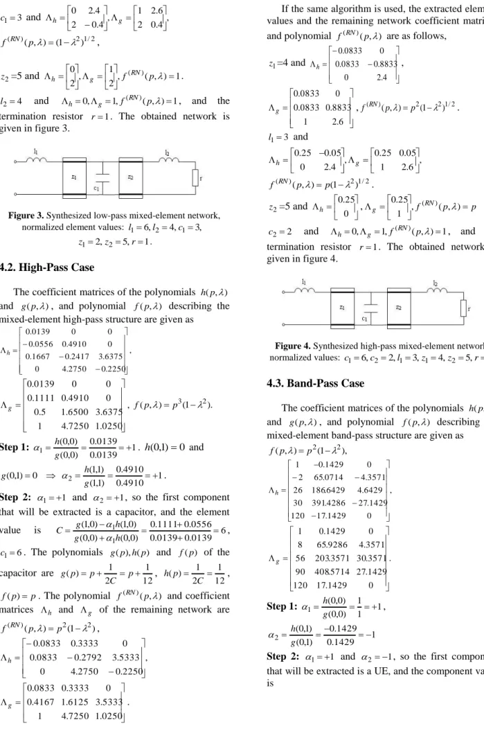
Figure 3. Synthesized low-pass mixed-element network, normalized element values: l16,l24,c13,

1 , 5 , 2 2 1 z  r z .

4.2. High-Pass Case

The coefficient matrices of the polynomials h(p,) and g(p,), and polynomial f(p,) describing the mixed-element high-pass structure are given as

, 2250 . 0 2750 . 4 0 6375 . 3 2417 . 0 1667 . 0 0 4910 . 0 0556 . 0 0 0 0139 . 0                   h , 0250 . 1 7250 . 4 1 6375 . 3 6500 . 1 5 . 0 0 4910 . 0 1111 . 0 0 0 0139 . 0                g f(p,)p3(12). Step 1: 1 0139 . 0 0139 . 0 ) 0 , 0 ( ) 0 , 0 ( 1   g h  . h(0,1)0 and  0 ) 1 , 0 ( g 1 4910 . 0 4910 . 0 ) 1 , 1 ( ) 1 , 1 ( 2   g h  .

Step 2: 11 and 21, so the first component

that will be extracted is a capacitor, and the element

value is 6 0139 . 0 0139 . 0 0556 . 0 1111 . 0 ) 0 , 0 ( ) 0 , 0 ( ) 0 , 1 ( ) 0 , 1 ( 1 1 _       h g h g C   , 6 1

c . The polynomials g(p),h(p) and f( p) of the capacitor are 12 1 2 1 ) (   p C p p g , 12 1 2 1 ) (   C p h , p p

f( ) . The polynomial f(RN)(p,) and coefficient matrices h and g of the remaining network are

) 1 ( ) , ( 2 2 ) ( _{  } p p f RN , , 2250 . 0 2750 . 4 0 5333 . 3 2792 . 0 0833 . 0 0 3333 . 0 0833 . 0               h             0250 . 1 7250 . 4 1 5333 . 3 6125 . 1 4167 . 0 0 3333 . 0 0833 . 0 g .

If the same algorithm is used, the extracted element values and the remaining network coefficient matrices and polynomial f(RN)(p,) are as follows,

1 z =4 and               4 . 2 0 8833 . 0 0833 . 0 0 0833 . 0 h ,             6 . 2 1 8833 . 0 0833 . 0 0 0833 . 0 g , 2 / 1 2 2 ) ( ) 1 ( ) , (p p  f RN . 3 1 l and , 6 . 2 1 05 . 0 25 . 0 , 4 . 2 0 05 . 0 25 . 0                 _{h g} 2 / 1 2 ) ( ) 1 ( ) , (p p  f RN . 2 z =5 and _        0 25 . 0 h , f p p RN g          , ( , ) 1 25 . 0 _{( )}  2 2

c and _h0,_g1,f(RN)(p,)1, and the termination resistor r1. The obtained network is given in figure 4.

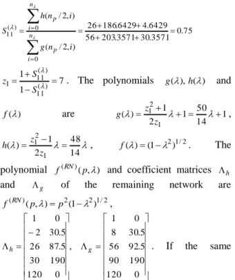
Figure 4. Synthesized high-pass mixed-element network, normalized values: c16,c22,l13,z14,z25,r1.

4.3. Band-Pass Case

The coefficient matrices of the polynomials h(p,) and g(p,), and polynomial f(p,) describing the mixed-element band-pass structure are given as

), 1 ( ) , (p p2 2 f , 0 1429 . 17 120 1429 . 27 4286 . 391 30 6429 . 4 6429 . 186 26 3571 . 4 0714 . 65 2 0 1429 . 0 1                       _h . 0 1429 . 17 120 1429 . 27 5714 . 408 90 3571 . 30 3571 . 203 56 3571 . 4 9286 . 65 8 0 1429 . 0 1                  _g Step 1: 1 1 1 ) 0 , 0 ( ) 0 , 0 ( 1   g h  , 1 1429 . 0 1429 . 0 ) 1 , 0 ( ) 1 , 0 ( 2     g h 

Step 2: 11 and 2 1, so the first component

that will be extracted is a UE, and the component value is

75 . 0 3571 . 30 3571 . 203 56 6429 . 4 6429 . 186 26 ) , 2 / ( ) , 2 / ( 0 0 ) ( 11 _{ }     





     n i p n i p i n g i n h S 7 1 1 ) ( 11 ) ( 11 1     _ S S

z . The polynomials g(),h() and

) ( f are 1 14 50 1 2 1 ) ( 1 2 1  _{  }     z z g ,    14 48 2 1 ) ( 1 2 1  _  z z h , f()(12)1/2. The

polynomial f(RN)(p,) and coefficient matrices _h and g of the remaining network are

2 / 1 2 2 ) ( ) 1 ( ) , (p  p  f RN ,                                      0 120 190 90 5 . 92 56 5 . 30 8 0 1 , 0 120 190 30 5 . 87 26 5 . 30 2 0 1 g h . If the same

algorithm is used, the extracted element values and the remaining network coefficient matrices and polynomial

) , ( ) ( _ p f RN are as follows, 1 l =4and , 180 30 5 . 92 36 5 . 30 8 0 1 , 180 30 5 . 87 6 5 . 30 2 0 1                                  _{h g} 2 / 1 2 2 ) ( ) 1 ( ) , (p  p  f RN 5 1 c and , 36 6 5 . 18 6 6 1 , 36 6 5 . 17 0 6 1                          _{h g} 2 / 1 2 ) ( ) 1 ( ) , (p p  f RN 2 z =6 and , 6 6 1 , 6 0 1                        h g f(RN)(p,)p. 3 2 l and , ( , ) 1 1 1 , 1 0 _{( )}                  h g f RN p , 2 2

c and h0,g 1,f(RN)(p,)1, and the termination resistor r1. The obtained network is given in figure 5.

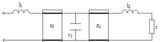
Figure 5. Synthesized band-pass mixed-element network , normalized values: 1 , 2 , 5 , 3 , 4 , 6 , 7 _{2 1 2 1 2} 1 z  l  l  c  c  r z .

4.3. Band-Stop Case

The coefficient matrices of the polynomials h(p,) and g(p,), and polynomial f(p,) describing the mixed-element band-stop structure are given as

, 6 . 264 8 . 793 0 2 . 427 6 . 138 24 4 . 50 2 . 163 6 2 . 11 1 . 5 2 05 . 1 15 . 3 0                         h , 4 . 365 2 . 970 252 2 . 427 6 . 306 60 6 . 69 8 . 196 54 2 . 11 1 . 9 4 45 . 1 85 . 3 1                  g ). 1 )( 004 . 0 1905 . 0 ( ) , (p  p4 p2 2 f Step 1:h(2,0)60 11, 1 2 . 11 2 . 11 ) 2 , 1 ( ) 2 , 1 ( 2    g h  .

Step 2: 11 and 2 1, so the first component

that will be extracted is a UE, and the component value is 3333 . 0 6 . 69 8 . 196 54 4 . 50 2 . 163 6 ) , 2 / ( ) , 2 / ( 0 0 ) ( 11 _{ }      





     n i p n i p i n g i n h S , 2 1 1 ) ( 11 ) ( 11 1     _ S S

z . The polynomials g(),h() and

) ( f are 1 4 5 1 2 1 ) ( 1 2 1  _{  }     z z g ,    4 3 2 1 ) ( 1 2 1  _  z z h , f()(12)1/2. The

polynomial f(RN)(p,) and coefficient matrices _h and g of the remaining network are

2 / 1 2 2 4 ) ( ) 1 )( 004 . 0 1905 . 0 ( ) , (p  p  p   f RN ,                                          2 . 655 252 6 . 213 60 8 . 124 54 6 . 5 4 6 . 2 1 , 8 . 604 0 6 . 213 24 2 . 115 6 6 . 5 2 4 . 2 1 g h . If the same

algorithm is used, the extracted element values and the remaining network coefficient matrices and polynomial

) , ( ) ( _ p f RN are as follows, 1 l =3 and c12, , 2 . 109 42 6 . 0 3 6 . 2 1 , 8 . 100 0 6 . 0 3 4 . 2 0                         _{h g} 2 / 1 2 2 ) ( ) 1 )( 42 1 ( ) , (p  p   f RN , 2 z =5 and , 42 3 1 , 0 3 0                        _{h g} ) 42 1 ( ) , ( 2 ) ( _{ } p p f RN  . 6 2  l and c27 and 1 ) , ( , 1 , 0  ( )  

_{h g} f RN p  , and the termination resistor r1. The obtained network is given in figure 6.

Figure 6. Synthesized band-stop mixed-element network, normalized values: 1 , 7 , 2 , 6 , 3 , 5 , 2 _{2 1 2 1 2} 1 z  l  l  c  c  r z .

5. Conclusions

The unavoidable connections between elements destroy the performance of the lumped-element networks at high frequencies. But these connection lines can be used as circuit components. In this case, the circuits must be composed of mixed lumped and distributed elements. But a complete theory for the approximation and synthesis problems of mixed-element networks is still not available.

In this paper, synthesis of lossless ladder networks with simple lumped elements connected with UEs is examined. The synthesis of mixed-element networks may be realized by using single variable boundary

polynomials, namely the polynomials

) 0 , ( ), 0 , ( ), 0 , (p g p f p

h for lumped-element section, and ) , 0 ( ), , 0 ( ), , 0 (  g  f 

h for distributed-element section

[11-12]. In this case, synthesis is carried out for lumped and distributed sections separately. Then, the components are mixed, to construct the mixed-element network. But in the presented algorithm, the synthesis of mixed-element network is carried out directly by using the two-variable reflection function of the mixed-element network, and components are extracted according to the connection order in the mixed-structure. The implementation of the proposed algorithms is utilized by the given examples. As a result, simple mixed-element network synthesis algorithm has been presented, which is necessary for the applications using this ladder-type of mixed-element networks, e.g. design of filters, broadband matching networks and amplifiers [13-15].

6. References

[1] B.K. Kinariwala, “Theory of cascaded structures: lossless transmission lines”, Bell Syst Tech. J., vol.45, pp.631-649, 1966.

[2] L.A. Riederer, L. Weinberg, “Synthesis of lumped-distributed networks: lossless cascades”, IEEE Trans

CAS, vol.27, pp.943-956, 1980.

[3] P.I. Richards, “Resistor transmission line circuits”, Proc

IR, vol.36, pp.217-220, 1948.

[4] H. Ozaki, T. Kasami, “Positive real functions of several variables and their applications to variable networks”,

IEEE Trans Circuit Theory, vol.7, pp.251-260, 1960.

[5] B.S. Yarman, A. Aksen, “An integrated design tool to construct lossless matching networks with mixed lumped and distributed elements”, IEEE Trans CAS, vol.39, pp.713-723, 1992.

[6] A. Aksen, “Design of lossless two-port with mixed, lumped and distributed elements for broadband matching”, PhD Thesis, Ruhr University, 1994.

[7] A. Aksen, B.S. Yarman, “A real frequency approach to describe lossless two-ports formed with mixed lumped and distributed elements”, Int J Elec Comm (AEU), vol.55(6), pp.389-396, 2001.

[8] A. Sertbaş, B.S. Yarman, “A computer aided design technique for lossless matching networks with mixed lumped and distributed elements”, Int J Elec Comm

(AEÜ), vol.58, pp.424-428, 2004.

[9] M. Şengül, “Construction of lossless ladder networks with simple lumped elements connected via commensurate transmission lines”, IEEE Trans.

CAS-II:Express Briefs, vol.56(1), pp.1-5, 2009.

[10] A. Sertbaş, “Genelleştirilmiş iki-kapılı, iki-değişkenli kayıpsız merdiven devrelerin tanımlanması” (in Turkish), PhD Thesis, Istanbul University, 1997. [11] M. Şengül, “Synthesis of cascaded commensurate

transmission lines”, IEEE Trans CAS-II:Express Briefs, vol.55(1), pp.89–91, 2008.

[12] M. Şengül, “Explicit synthesis formulae for cascaded lossless commensurate lines”, Frequenz, vol.62(1-2), pp.16-17, 2008.

[13] M. Şengül, B.S. Yarman, “Design of broadband microwave amplifiers with mixed-elements via reflectance data modelling”, Int J Elec Comm (AEU), vol.62(2), pp.132-137, 2008.

[14] M. Şengül, “Modeling based real frequency technique”,

Int J Elec Comm (AEU), vol.62(2), pp.77-80, 2008.

[15] M. Şengül, “Design of broadband single matching networks”, Int J Elec Comm (AEU), vol.63(3), pp.153-157, 2009.

Metin Şengül received his B.Sc. and M.Sc. degrees in Electronics Engineering from Istanbul University, Turkey in 1996 and 1999, respectively. He completed his Ph.D. in 2006 at Işık University in Istanbul, Turkey. He worked as a technician at Istanbul University from 1990 to 1997 and was a circuit design engineer at the R&D Labs of the Prime Ministry Office of Turkey between 1997 and 2000. He was employed as a lecturer and assistant professor at Kadir Has University, Istanbul, Turkey between 2000 and 2010. Dr. Şengül was a visiting researcher at the Institute for Information Technology, Technische Universität Ilmenau, Ilmenau, Germany in 2006 for six months. Currently, he is an associate professor at Kadir Has University, Istanbul, Turkey and working on microwave matching networks/amplifiers, device modeling, circuit design via modeling and network synthesis.