Performance of orbital angular momentum based communication systems under varied atmospheric turbulence

(1)

KADIR HAS UNIVERSITY

GRADUATE SCHOOL OF SCIENCE AND ENGINEERING

Performance of Orbital Angular Momentum Based Communication

Systems under varied Atmospheric Turbulence

Abdul Ahad Ashfaq Sheikh

(2)

ABDU L A HA D ASHF AQ S HE IK H Ma ster The sis 2016

(3)

C

Performance of Orbital Angular Momentum Based Communication

Systems under varied Atmospheric Turbulence

ABDUL AHAD ASHFAQ SHEIKH

B.E., Electronics Engineering, National University of Sciences and Technology, Pakistan

,

2012

M.Sc., Electronics Engineering, Kadir Has University, 2016

Submitted to the Graduate School of Science and Engineering

In partial fulfillment of the requirements for the degree of

Master of Science

Electronics Engineering

KADIR HAS UNIVERSITY September, 2016

(4)

(5)

(6)

(7)

(8)

i

Performance of Orbital Angular Momentum Based Communication

Systems under varied Atmospheric Turbulence

Abstract

Orbital Angular Momentum is gaining a lot of attention in the past years as it is providing the means to break free from the ever increasing shortage of options when it comes to Data Rates and Effective Frequency Utilization. OAM promises to break the shackles and provide a solution where a beam which can be transformed into multiple beams within itself and become independent streams of data (pertaining to the principle of orthogonality) to be transferred when properly utilized. In this thesis the generation of these beams is discussed along with how to propagate them through free space and send and receive data. As astonishing as it seems there is a draw back in reality from theory. Free space contains Atmospheric Turbulence which interferes with the beam propagation of OAM and as a result the photons in the light beam are affected as well as the independence of each OAM mode is affected. Accordingly, the data stream suffers crosstalk. In this thesis Weak and Strong Atmospheric Turbulences and how they effect a variety of OAM modes as they propagate through free space are studied a comparison between them are provided.

Keywords: Orbital Angular Momentum, Atmospheric Turbulence, Data Rates, Frequency Utilization, Cross Talk, Interference, Orthogonality.

(9)

ii

Yörüngesel Açısal Momentum Tabanlı Haberleşme Sistemlerinin

Değişik Atmosfer Türbülansındaki Performansı

Özet

Yörüngesel Açısal Momentum (OAM) son yıllarda yüksek veri hızı ve verimli frekans kullanımı açılarından oldukça dikkat çekmektedir. OAM tek bir ışık hüzmesinin çoklu bağımsız ışık hüzmeleri olarak iletimi üzerinedir. Bu tezde ışık hüzmelerinin oluşturulması, iletilmesi ve alınması incelenmiştir. Gerçek yaşamda ışık hüzmeleri ve fotonlar Atmosfer Türbülansı tarafından etkilenir ve bu da OAM modlarının bağımsızlığını etkiler. Bunun sonucu olarak da veri iletiminde çapraz karışmaya neden olur. Bu tezde Güçsüz ve Güçlü Atmosfer Türbülansı’nın OAM modlarına etkileri incelenmiş ve karşılaştırmalı sonuçlar sunulmuştur.

Anahtar Sözcükler: Yörüngesel Açısal Momentum, Atmosfer Türbülansı, Veri Hızları, Frekans Kullanımı, Çapraz Karışma, Girişim, Diklik

(10)

iii

Acknowledgements

First and foremost, by the grace of the Almighty I was able to undertake such a demanding task and able to fulfill its requirements as well.

I would like to thank the guiding brain behind this thesis, my supervisor, Assoc. Prof. Dr. Serhat Erkucuk who never lost hope in my abilities and always kept me motivated to attain my goals through his expertise and prowess. I appreciate the time and effort you put in to make this happen. Thank You Sir!

I would like to thank my friends Abdur Rehman bin Tahir, Mohammad Sohaib, Rameez Ahmed Samo and Ahmed Saad for being a great support in times of utter hopelessness.

My family who have always been there for me and made me believe that I can achieve what I set out to achieve and lastly I would like to thank my Father, Air Commodore (R) Muhammad Ashfaq Sheikh who has always been the guide and the shining light to inspire me to work hard diligently.

(11)

iv

Dedication

(12)

v

List of Figures

Figure1.1: SAM and OAM……….2

(14)

vii

Figure 2.1: Gaussian Beam and LG beam with m=1 ... 9

Figure 2.2: Gaussian beam passed through diffraction pattern ... 10

Figure 2.3: Gaussian Beam passing through diffraction pattern with induced OAM m=3 [3] ... 11

Figure 2.4: OAM +3 mode profile [Array Calc v2.5 Matlab Toolbox]... 11

Figure 2.5: Depiction of SPP producing OAM ... 12

Figure 2.6: OAM phase accumulation ... 14

Figure 2.7: OAM depiction through LG Beam phase ... 15

Figure 2.8: First 16 LG OAM modes ... 15

Figure 4.1: Constellation of OAM modes through complex AWGN ... 25

Figure 4.2: Constellation point scattering due to 𝐶_𝑛2 _{= 10}−16_{... 26}

Figure 4.3: Constellation point scattering due to 𝐶𝑛2 = 10−15 ... 26

Figure 4.4: Constellation point scattering due to 𝐶𝑛2= 10−14 ... 27

Figure 4.5: 3D view of detection probability with weak turbulence... 28

Figure 4.6: 2D view solidifying for like behavior of scattering by weak turbulence 28 Figure 4.7: 3D view of detection probability with strong turbulence ... 29

(15)

viii

Figure 4.9: Probability of reception of m through weak turbulence, Johnson-SB

distribution ... 30

Figure 4.10: Surface plot for OAM modes through Weak Atmospheric Turbulence ... 31

Figure 4.11: Probability of reception of m=0 ... 31

Figure 4.13: Probability of reception of m through high turbulence 𝐶_𝑛2 = 10−14 ... 33

Figure 4.14: Surface plot portraying detection chances of modes -9 to 20 with y axis representing matrix number. ... 34

(16)

ix

List of Tables

Table 3.1: Weak Turbulence Diagonal Element Distribution ... 22

Table 3.2:Weak Turbulence Off Diagonal Element Distribution ... 22

Table 4.1: Reception with conditional probabilities for modes in strong turbulence 37 Table 4.2: Probability of correct reception with combined modes at different rates………38

Table A.1Strong Turbulence Matrix (m= 0 to 20, n= -9 to 0)……….47

Table A.2Strong Turbulence Matrix (m= 0 to 20, n= 1 to 11)………48

Table A.3 Strong Turbulence Matrix (m= 0 to 20, n= 12 to 20)………49

Table A.4 Weak Turbulence Matrix (m= 0 to 9, n= 0 to 9)………50

List of Abbreviations

OAM Orbital Angular Momentum

SAM Spin Angular Momentum

OFDM Orthogonal Frequency Division Multiplexing

LG Laguerre Gaussian

(17)

x 4G 4th Generation

LTE Long Term Evolution

SPP Spiral Phase Plates

SLM Spatial Light Modulators

CAGR Compound Annual Growth Rate

GB Gigabyte

(18)

1

Chapter 1

1. Introduction

The world as we know it is going through a technological boom, as cliché as it must sound in the fields of Engineering, Biology, Physics, Astronomy to name a few are impacting how we live our lives every day. The information that keeps on piling up for us to utilize and benefit from to further gasp in amazement into the spiral of curiosity and day by day defy the odds and achieve the extraordinary from the ordinary that we thought of just yesterday.

The world of communications has come a long way with the help of its sister fields of hardware and radio communications. From a mere modest radio message scouring the earth’s atmosphere to secured channel transmissions that travel the air, the sea and land. Just when we think the human race has achieved its pinnacle we push even further.

The fact that is being dwelled upon here is a discovery so surprising that it has revolutionized how we would think about information transmission in the future. From the first radio signal transmitted and received in 1901 by Marconi [1] to the discovery of shaft like motion of a wave by Dr. Poynting in 1909 [2], the world of engineering was bedazzled by a discovery by Allen et al in 1992 that light constituting photons not only has linear momentum equivalent to ħ𝑘0 per photon

[3] in it if linearly polarized as a physical quantity but also has a shaft like motion that when properly induced can attain spin and orbital momentum in it as well equivalent to ±ħ per photon. Giving rise to Spin Angular Momentum (SAM) and Orbital Angular Momentum (OAM), which induces a torque, that can be used to move infinitesimal objects or rotate them as illustrated in Fig 1.1. An interesting consequence could lead to turning a door knob in the future [3]. Laser beams have

(19)

2

been used to demonstrate the said effect using proper construction, explained later, but it’s better to refer to these beams as light. The build up to this point refers to the application of this discovery in communications engineering. What this wonder has enabled us to do is increase our capacity to ride data on a carrier. In this case light! Astonishing isn’t it?

Figure 1.1: SAM and OAM [3]

With the discovery of OAM, we are able to understand that light when properly polarized or ‘twisted’ in its phase property through special means produces infinite number of replica of the very same light. This is actually the same light but split into different phases which are totally orthogonal to each other leading to the fact that these entities or derivations do not interfere with each other. Subsequently providing us with the opportunity to ride data on them independent of each other. This means an infinite number of data streams can be carried through one light beam/carrier theoretically. Which is enabled by the property of a light beam being manipulated by a single factor that light beams with an azimuthal phase dependence of 𝑒𝑖𝑙∅ can carry OAM which can be many times greater than the SAM [3]. But as we propagate these beams through Free-Space we suffer a drastic hit to our theory and the independent ‘modes’ of each beam start to interfere with each other which we will discuss in detail in this thesis. Furthermore, how the Atmospheric

(20)

3

Turbulence affects the modes transmitted and the data within will be demonstrated. In Fig 1.2 different OAM modes are depicted.

Figure 1.2: OAM modes (0-3), LG beam

As a result, we end up creating channels for our data to pass through. This discovery has enabled us to gear up for the ever increasing demand for high data rates and using less bandwidth to provide an equivalently larger order of bandwidth for data transmission. With this possibility we are able to address the ever increasing demand for a solution to congestion and running out of frequency spectrum to propagate wireless communications as well as the limits we face with wired transmission technologies as well. Not only this solution will allow for the modern communication engineer to design and provide high bandwidth, capacity, data rates and security to data networks but also revolutionize how we think about the current flow of information and its access. Mobile data traffic has grown 4,000-fold over the past 10 years and almost 400-million-fold over the past 15 years. Mobile networks carried fewer than 10 gigabytes per month in 2000, and less than 1 petabyte per month in 2005. (One Exabyte is equivalent to one billion gigabytes,

(21)

4

and one thousand petabytes.) [4]. Fourth-generation (4G) traffic exceeded third-generation (3G) traffic for the first time in 2015. Although 4G connections represented only 14 percent of mobile connections in 2015, they already account for 47 percent of mobile data traffic, while 3G connections represented 34 percent of mobile connections and 43 percent of the traffic [4]. In 2015, a 4G connection generated six times more traffic on average than a non 4G connection. Global mobile data traffic will increase nearly eightfold between 2015 and 2020. Mobile data traffic will grow at a compound annual growth rate (CAGR) of 53 percent from 2015 to 2020, reaching 30.6 Exabyte’s per month by 2020. [4]

To reach these goals, OAM is an important candidate. Next, a literature review, on OAM and the effects of Atmospheric Turbulence are presented.

1.1 Literature Review

This technology OAM has recently come to limelight as researchers and physicists and engineers have recently started taking interest in the many marvels this technology has to offer. Moving on from techniques like Frequency Division Multiplexing (FDM) [5], Orthogonal Frequency Division Multiplexing (OFDM) [5], Global System for Mobile Communications (GSM), 2G, 4G and Long Term Evolution (LTE) just to name a few OAM has a lot to offer when it comes to Communications and Wireless Communications to be specific [6] [7] [8].

The world is changing fast and since the experiments that boost the trust in communications and new techniques [6] there is certainly a way forward [3] for OAM. Work is underway to come up with more customized modulation formats to support OAM [9]. The spectral efficiency is being increased using these modulation techniques as they are deemed multidimensional incorporation more data and allowing more freedom [9] [10] [11]. A recent experiment has boasted a

(22)

5

demonstrate a 32-Gbit/s millimeter-wave link over 2.5 meters with a spectral efficiency of 16 bit/s/Hz using four independent OAM beams on each of two polarizations. All eight orbital angular momentum channels are recovered with bit-error rates below 3.8𝑥10−3_{[12]. Scientists are also launching studies into catering}

for increasing the channel capacity as to come up with ways to attain the best modes to transmit and also enhance their capability to carry data. An experiment to carry a terabit of data has also been conducted which further backs up the credibility of the technology to take on the future [13]. There have also been advancements into modelling the Atmospheric Turbulence a bit more and to provide better capacity to the channel [14].

The use of Spatial Light Modulators (SLM) has impacted the work a lot as we see that these modulators use the beams being fed to them and multiplex the beam in a way to provide for optical modulation as a good way to attain the multiplexing phenomenon and are very useful in laboratory environments [15]. Phase Screens are used at equivalent intervals to simulate different Atmospheric disturbances to light which have helped us attain the desired effect in order to disturb the transmitting powers and receive the mode transmission to attain the desired detection/reception probabilities [11] [14] [16].

There have been similar ways to understand effects of turbulence on constellation points which help us understand the relation to modes graphically in a trend [17] [18] [19] along with higher mode detection. There have certainly arisen some encoding techniques which support the fact for a complete package for OAM as the future which allow for better error rates and transmissions [20] [21]. As was described that the higher the modes the difficult for them to be distinguished between each other a good approach to how that can be done has also been

(23)

6

explained which works very well in tandem with our approach as well [20]. The most popular Quadrature Phase Shift Keying (QPSK) is gaining a lot of use in tandem with OAM [22]. A great guide to a primer for OAM beginners is certainly recommended to read in [3] as it would help the new and upcoming researchers to gear up for the technology.

Motivated by not concentrated studies on the Effect of Atmospheric Turbulence on OAM based communication and by the lack of appropriate mathematical models from the communication perspective (most works on OAM are experimental based), we provide a comprehensive study on the performance of OAM for various Atmospheric Turbulence models in this thesis. The results provided are important for understanding the effect of atmospheric turbulence from the communication perspective. Next, the thesis organization is presented.

1.2 Thesis Organization

This thesis has been divided into 3 main parts. In the first part (Chapter 2), the mathematical model regarding OAM and the basics of a Gaussian Beam will be explained. Then various generation techniques of OAM will be briefly explained and the ones used will be indicated. Finally, how OAM beams attain orthogonality which is the basis for us to use them as a data channel for data transmission will be shown.

In the second part, (Chapter 3), how OAM reacts or propagates through Free Space and the effects of the Atmospheric Turbulence on data carrying streams will be explained. Under which different models of Atmospheric Turbulence will be discussed deeming them as Weak or Strong Turbulence.

(24)

7

In the third part (Chapter 4), effects on a given OAM beam and its modes due to the varieties of Atmospheric Turbulence experienced will be presented.

Afterwards, concluding remarks and possible extensions of the current work will be presented in Chapter 5.

(25)

8

Chapter 2

2. Mathematical Model of OAM

In this chapter the mathematical models regarding the OAM beam, how it has been derived and what modifications are done to a simple light beam will be discussed [23] [24] [25].

A brief explanation of the term OAM will be given followed by the different production techniques, the orthogonality of beams to provide for data transmission and the system model for the study conducted.

2.1 Orbital Angular Momentum (OAM)

Light is an integral part of our everyday life as it illuminates objects that allow us to see and visualize. The visible light spectrum is a collection of electromagnetic radiations visible to the human eye. What OAM proposes is that given the visible light and to be more specific for a Gaussian Beam we ‘twist’ or bend light in a specific way to manipulate its phase and in turn create an independent mode which occupies the same space as the beam, in turn giving us the liberty to create infinite independent instances of the beam and use it as a channel to transfer those ‘modes’ that we just created. The property 𝑒𝑖𝑙∅_{allows us to develop on that. The ′𝑙′ or ′𝑚′}

as we refer to in this thesis is identified as the topological charge which can have any integer value with a + or a – sign indicating the directional trend of the mode in the beam as it takes up a helical form [12].

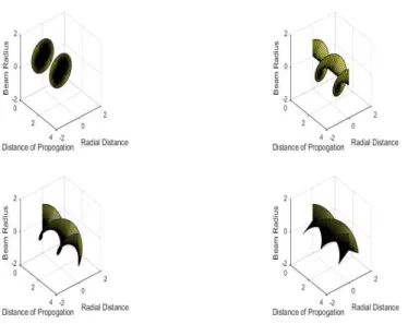
The OAM beam is considered to be a Gaussian Vortex beam as in has a hole in the center like a doughnut and then as modes are increased the rings/spirals start to develop up on its circumference indicating a new mode being added and so on and so forth [23] [24] as shown in Fig 2.1.

(26)

9

Figure 2.1: Gaussian Beam and LG beam with m=1

OAM has provided a platform to set free the radio spectrum deadlock being currently face by the Communications Engineers and also helps shed a light that a way forward does exist which can cope to our ever increasing cellular needs and also the data hungry and time sensitive networks all around the world. OAM is a great contender for future integrations to communications networks due to its many advantages explained earlier.

2.2 OAM Generation Techniques

As described earlier that OAM is derived from light and the spin on its photons. There are many techniques which help to create the phenomenon and here they will be explained briefly as follows.

2.2.1 Holograms/Diffraction Patterns

Holograms are generated through computers which act as a mesh of a grid through where light can be shone on and depending on the incidence angle and the distance

(27)

10

it has been shone on to the hologram dictates what pattern is developed as a result [3] [26] [28]. One such experiment is conducted and the result is shown in Fig. 2.2.

Figure 2.2: Gaussian beam passed through diffraction pattern

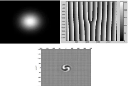
The pattern basically acts as a fork grating and twists the incoming beam with the correct parameters to achieve a desired result. The same can be done with a hologram which nullifies a phase and lets through another under observation e.g. in the diagram below, Fig 2.3. A simple Gaussian Beam travels and is incident on the hologram/diffraction pattern and a result is obtained in this case 𝑙=+3. They can be produced by computer programs and then developed onto photographic films, Gaussian or Laser Beams can be shone onto the material and the desired results obtained.

(28)

11

Figure 2.3: Gaussian Beam passing through diffraction pattern with induced OAM m=3 [3]

Figure 2.4: OAM +3 mode profile [Array Calc v2.5 Matlab Toolbox]

Fig 2.4, shows an OAM beam produced with m=+3 as it shows three phase accumulations and the trend of the modes being to the right.

(29)

12

2.2.2 Spiral Phase Plates

Spiral Phase plates act in the same way as do Diffraction/Hologram patterns, except the fact that they are made from materials specially produced in Labs to attain the desired effects. They are spiral plates as the name suggests they start off as being very thin as we move through the circumference and start to get thicker as we go on, as a result taking up a shape of somewhat a revolving shaft that increases in thickness as it revolves. When Beams are incident on the material the thinner part has less diffraction and the thicker parts have more. As a result, the phase changes are proportional to the thickness and we obtain higher order modes from thicker parts and lower order modes from the thinner parts. The optical thickness of the medium increases with azimuthal position according to 𝑙λ𝜃/2𝜋(𝑛 − 1)where n is the refractive index of the medium. They are generally created from crystal, plastic, High Density Polyethene [12] [28] etc. Spiral Phase Plate Generation of OAM is depicted in Fig 2.5 [3].

Figure 2.5: Depiction of SPP producing OAM [3] 2.2.3 Laguerre Gaussian Beams

The important fact that OAM is readily generated through Laguerre Gaussian beams has helped communication engineers a lot. Helically phased light carries

(30)

13

OAM irrespective of the radial distribution of the beam. However, it is useful to express most of beams in a complete basis set of orthogonal modes [18]. For OAM we therefore use LG mode set in this thesis. The best field distribution is described in cylindrical modes. For a radial distance ‘r’ from the propagation axis, azimuthal angle ‘∅’ and propagation distance ‘z’, the field distribution is described [11] [14] [18] as: 𝒖(𝒓, ∅, 𝒛) = √_{𝝅(𝒑+|𝒎|)!}𝟐𝒑! _𝒘(𝒛)𝟏 [𝒓√𝟐 𝒘(𝒛)] |𝒎|_𝒙𝑳 𝒑 𝒎_[ 𝟐𝒓𝟐 𝒘𝟐_(𝒛)] 𝒙 𝐞𝐱𝐩 [ −𝒓𝟐 𝒘𝟐_(𝒛)] 𝒙 𝐞𝐱𝐩 [ 𝒊𝒌𝒓𝟐𝒛 𝟐(𝒛𝟐_+𝒛 𝑹 𝟐₎] 𝒙 𝐞𝐱𝐩 [𝒊(𝟐𝒑 + |𝒎| + 𝟏)𝒕𝒂𝒏−𝟏 𝒛 𝒛𝑹] 𝐞𝐱𝐩 (−𝒊𝒎∅) (2.1)

where 𝑤(𝑧) = 𝑤₀√1 + (𝑧/𝑧𝑅)2 is the beam radius z, 𝑤0 is the radius of the

zero-order Gaussian Beam at the waist, 𝑧_𝑅 = 𝜋𝑤₀2/𝜋 is the Rayleigh Range, λ is the optical wavelength and 𝑘 = 2𝜋/λ is the propagation constant. The beam waist is at z= 0. The term 𝐿𝑚_𝑝represents the generalized Laguerre polynomial, and ‘p’ and ‘m’ are the radial and angular mode/topological charge numbers, respectively [11]. Also note the last member of the equation [3] was referred to earlier in the text to explain what brings about the OAM to life.

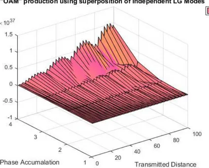
With the help of this equation we can produce an OAM mode to any extent that we want which will act as independent carriers of our data which we wish to transmit. As an experiment these equations have been simulated with different mode numbers ‘m’ and the rising phase trend has been observed as a result. Given that as the modes increase in the beam, the beam starts to grow and as the propagation distance is increased the beam grows.

(31)

14

Figure 2.6: OAM phase accumulation

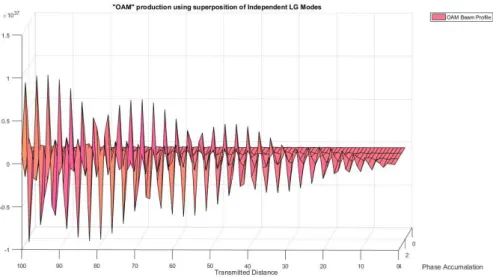
As a result, we can see in the Fig 2.6 that 3 modes are acting within the LG beam, and the trend of their phase is seen rising but also at the same time being incorporated in the same space as the whole group of phases taking off, as a result, producing OAM. Fig 2.7 shows the profile from a 2D perspective and helps understand the profile more readily.

(32)

15

Figure 2.7: OAM depiction through LG Beam phase

We can refer to Fig 1.2 to see how these modes are viewed individually. Also we can demonstrate the intensity profile of the beam as the LG beam with m=0 has a profile and when we rise in the integer value we see a ring shape forming for every new mode introduced in the beam [23] [24].

(33)

16

2.3 OAM Inter Mode Orthogonality

Given the background of how and why we use different techniques of producing OAM, further evidence will be demonstrated on how each mode is independent from each other. This quality of OAM has allowed to think of the possibilities pertaining to no interference between the modes, high data rates, effective bandwidth utilization, freedom from frequency spectrum deadlock [27].

What happens is that as many modes as we produce they will be orthogonal to each other and will not interfere with each other giving us the option to ride the different modes as separate channels for the number of data streams we require corresponding to the modes. This incredible feature is the focus of the attention OAM is receiving recently as a replacement for the deadlock of the frequency spectrum. It is as if we have been granted a space where an infinite number of data stream at high speeds and data rates are able to fulfill our ever-growing networking needs. This phenomenon is proved as follows [11] [14] [19] [21].

Given the received field 𝑈_𝑛(𝑟, ∅, 𝑧) with OAM state ‘n’ and the analyzing field 𝑈𝑚∗(𝑟, ∅, 𝑧) (where the * indicates the complex conjugate) with OAM state m, the

‘𝑚𝑡ℎ_{’ channel output signal (observed at the detector of channel m) is [11]}

𝑈𝑛(𝑟, ∅, 𝑧). 𝑈𝑚∗ (𝑟, ∅, 𝑧) ≜

∫ 𝑟𝑑𝑟𝑑∅𝑈𝑛(𝑟, ∅, 𝑧)𝑈𝑚∗(𝑟, ∅, 𝑧)={

0 ∀ 𝑛 ≠ 𝑚

∫ 𝑟𝑑𝑟𝑑∅|𝑢𝑚(𝑟, ∅, 𝑧)|2 𝑛 = 𝑚 (2.2)

With this property two modes are certainly orthogonal to each other and the property holds. This property has been used in this thesis to send and detect the transmit powers of the signals or channels and develop a channel matrix depicting the probability of detection of each mode sent. However, this property does not

(34)

17

always hold due to Atmospheric Turbulence which will be explained in the upcoming chapter.

(35)

18

Chapter 3

3. Atmospheric Turbulence

As described earlier, the OAM modes are orthogonal to each other meaning an infinite number of streams can be transmitted. That is not the case when the propagation of OAM beams in free space optical communication environments. The earth’s atmosphere includes many gases and substances along with the Sun’s rays, where there may be changes in temperatures and pressures all around the earth. Atmospheric turbulence is, small-scale, irregular air motions characterized by winds that vary in speed and direction. Turbulence is important because it mixes and churns the atmosphere and causes water vapor, smoke, and other substances, as well as energy, to become distributed both vertically and horizontally [16]. These changes induce gusts of winds, dust, minute elementary objects etc. to roam around the atmosphere. As a result, the physical particle ‘photon’ described in the Introduction has to face problems. In its normal form the beam would just travel through an ideal link. However, when we talk about wireless communication links that have to travel some distance and disseminate important information we are faced with Atmospheric Turbulence which is known to interact with the photon and negatively affect it. Atmospheric Turbulence consists of small eddies of air, dust etc. which can be described as pockets which are randomly distributed across the atmosphere and affect the propagation of beams. In the following section, how atmospheric turbulences are modelled and what effects these models have on the beams are explained [16].

(36)

19

3.1 Types of Atmospheric Turbulence 3.1.1 Kolmogorov Model

The earth’s atmosphere is a medium whose refractive index is nearly unity. This allows to make only slight modifications to propagation models in vacuum propagation techniques. Initially, original analysis of turbulent flow by Kolmogorov is given, which eventually led to statistical models of the refractive-index variation. Perturbation theory is used with the model to solve Maxwell’s equations [29] to obtain useful statistical properties of the observation-plane optical field.

As optical waves propagate through the atmosphere, the waves are distorted by these fluctuations in refractive index. Recently much attention is being shifted to how to simulate this phenomenon correctly as it is very difficult to model the fluctuations of the refractive index at every point of propagation. Thus, an idea of the random phenomenon is presented as those eddies of air are statistically homogeneous and isotropic within small regions of space, meaning that properties like velocity and refractive index have stationary increments. In the turbulence model, the atmospheric turbulence also has a master key that governs the strength of the turbulence, where 𝐶_𝑛2_{is known as the refractive-index structure parameter,}

measured in 𝑚−2/3. Further details are advised to interested readers in [16]. The Kolmogorov Turbulence Model model follows as

ᶲ_𝑛𝐾(𝐾) = 0.033𝐶_𝑛2_𝐾−11

3 𝑓𝑜𝑟 1

𝐿0 ≪ 𝐾 ≪ 1

𝑙0

(3.1)

where k is the angular spatial frequency in rad/m. 𝐿0 is the outer scale, which

represents the height of the eddies in the order of meters and may take realistic values. On the other hand, 𝑙₀ is the lower scale, which represents how high above the ground the eddies start.

(37)

20

3.1.2 Von-Karman

The Von-Karman model tweaks the Kolmogorov model and shows how we can efficiently improve the agreement between theory and experimentation. It is given as [11]. ᶲ_𝑛𝑣𝐾(𝐾) = 0.033𝐶𝑛2 (𝐾2_+𝐾 02) 11 6 𝑓𝑜𝑟 0 ≤ 𝐾 ≪ 1 𝑙0 (3.2)

and the modified version as [11]

ᶲ_𝑛𝑀𝑣𝐾(𝐾) = 0.033𝐶_𝑛2 exp (−𝐾2/𝐾𝑚2) (𝐾2_+𝐾

02)11/6 𝑓𝑜𝑟 0 ≤ 𝐾 < ∞ (3.3)

where 𝐾_𝑚 = 5.92/𝑙₀ and 𝐾₀ = 2𝜋/𝐿₀. The modified Von Karman is the simplest model that includes effects of both inner and outer scales. Note that when 𝑙0 =0 and

𝐿₀ = ∞ are used, the modified Von Karman model reduces to the basic Kolmogorov Model.

3.1.3 Modified Kolmogorov

The model that has the characteristics of both the Kolmogorov and the Von-Karman model, which have been developed to further address the problem accurately, describes the interaction between optical beams and the atmospheric turbulence as. [14] [16] DK(|∆r|) = 6.88 (r r0) 5 3 (3.4)

where 𝑟₀ is the atmospheric coherence diameter and r represents the spatial distance separated by two points over a phase front [14] [16] .

(38)

21

Considering the power spectrum considered due to turbulence and the channel matrix for the strong disturbance case, the modified Kolmogorov Model used in this thesis is as follows [11] ∅(𝐾)= 0.033𝐶𝑛2(𝐾2+ 1 𝐿2₀) −11₆ 𝑓(𝐾, 𝐾𝑙) 𝑤𝑖𝑡ℎ 𝑓(𝐾, 𝐾𝑙) = exp (−𝐾2 𝐾_𝑙2) [1 + 1.802 ( 𝐾 𝐾𝑙) − 0.254(𝐾/𝐾𝑙) 7/6_]_(3.5)

where 𝐾𝑙= 3.3/𝑙0. The turbulence strength is controlled by using the refractive

index structure parameter and it signifies how strong the turbulence is. The typical values range from 10−17 𝑡𝑜 10−13 measured in 𝑚−2/3. In this thesis the 𝐶𝑛2 10−14

value, which depicts strong turbulence is used. The weak turbulence is modelled with SB-Johnson model where 𝐶_𝑛2 = 10−15. This model is used to create phase screens at different points of the propagation of the OAM beam and as a result distortion between the orthogonal modes is observed causing interference within these modes.

3.2 Weak Atmospheric Turbulence

As described above the atmospheric turbulence has many variations. Sometimes high and sometimes low, values are experienced. Therefore, in this study a scintillation channel is simulated which closely predicts what happens, as the atmospheric turbulence has a value of 𝐶𝑛2 = 10−15. The Weak Atmospheric

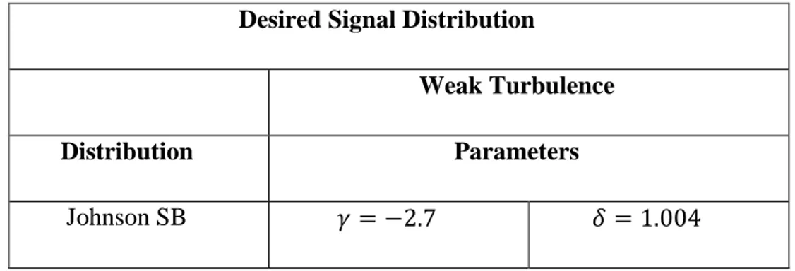
Turbulence has been modelled through the SB-Johnson statistic [21]. Here the channel is described as desired channel at the diagonal and interfering signals i.e. similar to Atmospheric Turbulence at the neighboring diagonals which will be exponentially distributed. Here the SB-Johnson model has been modeled using its parameters as shown in the table below. This conclusion has been derived through [11] [21]. The matrix representation of the problem is

(39)

22

𝐲 = 𝐇x + n (3.6)

where H is a transition matrix and all entries of the matrices are considered to be real [21].

Desired Signal Distribution

Weak Turbulence

Distribution Parameters

Johnson SB 𝛾 = −2.7 𝛿 = 1.004

Table 3.1: Weak Turbulence Diagonal Element Distribution

The entries of the neighboring diagonal are said to be interfering signals represented in the table below which will be exponentially distributed [21].

Interference Signal Distribution Weak Turbulence

Neighbor Distribution Parameters

First Exponential 1 𝜆=0.044 Second Exponential 1 𝜆=5𝑥10 −3 Third Exponential 1 𝜆=1.04𝑥10 −3

(40)

23

The effects of turbulence on the transmitted modes will be considered in the next chapter, where the results are averaged over 10,000 trials. We will compare it with experimental results of [11].

3.3 Strong Atmospheric Turbulence

Strong turbulence as explained earlier is modelled through the refractive index structure parameter. This value is taken to be 𝐶_𝑛2 = 10−14 OAM beams pass through the modified Kolmogorov Model [11] [14] [16]. The principle of orthogonality has been considered and the effect of turbulence has been assessed [11]. The received distorted OAM-carrying field is filtered according to the scalar product operation defined in Eq. 2.2 for every (m, n) and the result is normalized by the transmit optical power [11]. Since the distorted field is in fact a linear superposition of a number of OAM fields scaled by random scalar coefficients, what is recorded is the square of the normalized scalar product. This value represents the fraction of optical power observed in received OAM state n. The resulting projection for each (𝑚, 𝑛) corresponds to one instance of the channel. This operation is repeated for 10,000 different channel instances.

Ideally, the channel matrix would be an identity matrix which resembles a matrix with no atmospheric turbulence. Also it could be used as a comparison to a low refractive index structure parameter value such as 𝐶_𝑛2 = 10−16 in which case almost no orthogonality is lost between the modes. Same is the case with the weak atmospheric turbulence matrix above. The matrices in this study have been defined as powers populated against the sent and received modes and are compared as probabilities of reception between them [11].

(41)

24

Chapter 4

4. Effect of Atmospheric Turbulence on OAM modes.

In earlier chapters, mathematical model of OAM and the atmospheric turbulence were presented. In this chapter, the effect of atmospheric turbulence to different modes as they are propagated and what happens to their chances of being detected or received as they were sent are studied. Note that the ideal case was explained in the earlier chapter.

The OAM modes start to lose orthogonality as the modes have the tendency to shift to each other or as in technical terms crosstalk is induced in various channels. This crosstalk is harmful from the communication perspective. As propagating through free space, this challenge is faced therefore, through this study a way to identify which modes are best transmitted with their combinations and which models are suitable for transmission are presented.

We start by explaining the effects of the basic Von-Karman-Kolmogorov Modified Model [9] [17] [18] [19] on a constellation and then provide the comparison between the Johnson-SB model for weak turbulence and the Strong Turbulence using Modified Kolmogorov Model.

4.1 Kolmogorov Model Effect on a Constellation point

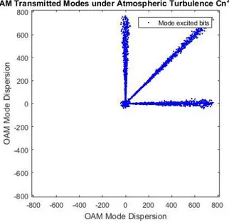
We generate a bit stream and then map it to corresponding mode numbers given a particular set of bits, e.g. a ‘00’ chunk describes a m=0 mode of OAM and ‘01’ describes that the first mode will go through. When we introduce this system to the Atmospheric Turbulence what we observe is that the constellation is scaled many a fold due to a scaling effect or dispersion of the modes observed with the Kolmogorov Model.

(42)

25

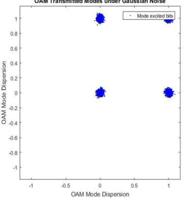
At first we present a constellation with coordinates as the 4 OAM mode possibilities to be transmitted, under normal Gaussian noise in Fig 4.1.

Figure 4.1: Constellation of OAM modes through complex AWGN

Secondly we show the effect of Atmospheric Turbulence with 𝐶𝑛2 = 10−16 in Fig

(43)

26

Figure 4.2: Constellation point scattering due to 𝐶𝑛2= 10−16

Then we show the effect with 𝐶𝑛2 = 10−15 in Fig 4.3 and with 𝐶𝑛2 = 10−14 in Fig

4.4. Note that these figures illustrate the effect of atmospheric turbulence for different levels at one constellation point. Further note that thresholds are not used to determine mode dispersions, where the figures are just illustrative.

(44)

27

Figure 4.4: Constellation point scattering due to 𝑪𝒏𝟐 = 𝟏𝟎−𝟏𝟒

These plots for the constellation show that if the OAM modes are transmitted, a dispersion is experienced depending on 𝐶_𝑛2_{. As the Atmospheric Turbulence gets}

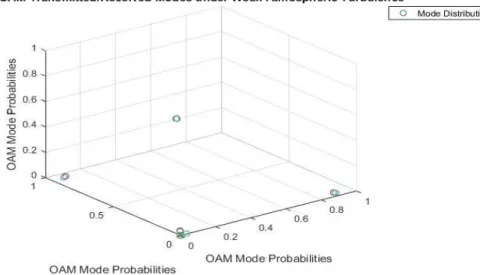
stronger the scattering takes a fork like shape to its destination mode and is scaled in a way. Therefore, it is concluded that one mode is scattered to many other modes due to the disturbance imitating the dispersion of phases of modes into other modes. As an example it is shown that when the transmitting powers are processed using the principle of orthogonality Eq. 2.2 and using the LG beam Eq. 2.1 as orthonormal basis also used in defining the coordinates and transmit powers [19] [21] it is observed that if the probabilities of the H matrix are scattered as explained later the trend they follow is the same as for the constellation scattering. This is shown below in Fig 4.5 to 4.8 for weak atmospheric turbulence and strong atmospheric turbulence.

(45)

28

Figure 4.5: 3D view of detection probability with weak turbulence

(46)

29

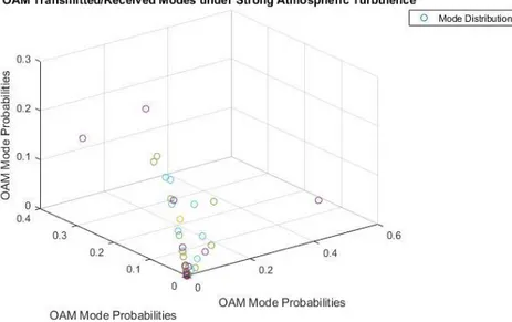
Figure 4.7: 3D view of detection probability with strong turbulence

Figure 4.8: 2D view for behavior of scattering by strong turbulence

This comparison is similar to the trend observed and helps to prove the turbulence effect on the constellation as well as the OAM modes.

(47)

30

4.2 Weak Atmospheric Turbulence Effect

For weak Atmospheric Turbulence, the Johnson-SB model is used to simulate weak turbulence. For modes 𝑚 ∈ {0,1, … ,9} , a 10x10 matrix shows crosstalk and the different probabilities of the transition matrix which depicts how well the OAM modes were received after going through atmospheric turbulence are plotted. This is presented in Fig 4.9.

Figure 4.9: Probability of reception of m through weak turbulence, Johnson-SB distribution

Here it can be seen that almost 91% correct reception is achieved but due to weak turbulence we see that the trend that theory predicted comes true, as higher modes are transmitted their probability of reception should be less (considering experimental results of [11]).

Due to weak Atmospheric Turbulence not much can be seen in the result and only a very minute fall in reception probabilities is seen.

0 0.2 0.4 0.6 0.8 1 0 1 2 3 4 5 6 7 8 9 Cros sta lk/Re cp tio n Pro b ab ili ty

Recieved OAM State Numbers

W E A K A T M O S P H E R I C T U R B U L E N C E R E C E P T I O N P R O F I L E

m=0 m=1 m=2 m=3 m=4 m=5 m=6 m=7 m=8 m=9

(48)

31

Figure 4.10: Surface plot for OAM modes through Weak Atmospheric Turbulence

We now show how different modes fare as we send m=0 in Fig

Figure 4.11: Probability of reception of m=0

This trend shows that after the third neighbor, no crosstalk modes are detected. This shows that the trend closely matches to the 𝐶_𝑛2 _{= 10}−15_{profile in [11]. Therefore,}

it can be safely said that the two models are comparable but the Johnson-SB model falls short of truly depicting how the Atmospheric Turbulence acts upon the OAM modes and their effect on the principle of orthogonality as the Johnson-SB distribution does not depend on m.

0 1 2 3 m=0 0.906267197 4.21E-02 4.98E-03 0.001038919 0 0.2 0.4 0.6 0.8 1 Cros sta lk/Re ce p tio n Pro b ab ili ty

Recieved OAM States

(49)

32

The Johnson-SB statistical distribution, has the ability to tweak the upper limit for its distribution which lies on the main diagonal elements of the H matrix for weak turbulence thus, has the ability to replicate any form of turbulence. Meaning experimental results can be matched by simulation of the Johnson-SB distribution as the matrix. The strong turbulence matrix can be matched through this but again it would be a way of replicating the experimental values but the distribution will not be as accurate as the results obtained, therefore Johnson-SB closely relates to the weak turbulence. Next, the strong atmospheric turbulence effect will be investigated

Figure 4.12: Probability of reception of m=1 4.3 Strong Atmospheric Turbulence Effect

In this part the effect of strong turbulence on OAM modes is described. The derivation for the effect has already been explained in the previous chapters. Different mode reception profiles and how the said effect of crosstalk is induced in other receiving modes under 𝐶𝑛2 = 10−14 will be presented, where we will refer to

𝐶𝑛2 = 10−14 as strong turbulence in this part [11] [21].

0 1 2 3 4

Series1 4.21E-02 0.905562 4.03E-02 4.95E-03 0.0010378 0.00E+00 2.00E-01 4.00E-01 6.00E-01 8.00E-01 1.00E+00 Cro sstalk/ Rec ep tio n P ro b ab ility

Recieved OAM States

(50)

33

Figure 4.13: Probability of reception of m through high turbulence 𝑪_𝒏𝟐 = 𝟏𝟎−𝟏𝟒

Here we can see a contrast in the reception profile as compared to weak atmospheric turbulence. This crosstalk is obtained from the H matrix as given in [11] and

0.00E+00 1.00E-01 2.00E-01 3.00E-01 4.00E-01 5.00E-01 6.00E-01 − 9 − 8 − 7 − 6 − 5 − 4 − 3 − 2 − 1 0 1 2 3 4 5 6 7 8 9 1 0 1 1 1 2 1 3 1 4 1 5 1 6 1 7 1 8 1 9 2 0 Cro ss tal k/Pro b ab ili ty o f De te cti o n

OAM Recieved States

R e c i e v e d O A M S t a t e P r o f i l e f o r S t r o n g T u r b u l e n c e

Received State 0 Received State 1 Received State 2 Received State 3 Received State 4 Received State 5 Received State 6 Received State 7 Received State 8 Received State 9 Received State 10 Received State 11 Received State 12 Received State 13 Received State 14 Received State 15 Received State 16 Received State 17 Received State 18 Received State 19 Received State 20

(51)

34

included in Appendix A. This shows that as higher order modes ‘m’ are transmitted there is lower possibility to detect them. The concept of crosstalk is induced and shown in Fig 4.15 below.

Figure 4.14: Surface plot portraying detection chances of modes -9 to 20 with y axis representing matrix number.

Next, individual modes and how they change by increasing the modes are presented in Fig 4.15 to 4.20

(52)

35

In these figures, how the Strong Atmospheric Turbulence is affecting the OAM modes is observed. It is seen that there is a drastic difference between the probabilities of reception. As with the weaker case clear outliers could be seen to the modes but with higher modes strong atmospheric turbulence causes neighboring modes to be detected. This was shown with the constellation point that as the turbulence increases the modes are dispersed and as a result the modes are interfering with each other. Furthermore, lower modes have better chances of detection compared to the higher modes when there is strong turbulence.

0.00659 0.0244 0.106 0.534 0.106 0.0244 0.00659 0 0.2 0.4 0.6 −3 −2 −1 0 1 2 3 Cros sta lk/Pro b ab ili ty o f d etection

Received OAM state number

m=0

0.00644 0.0162 0.0423 0.105 0.376 0.133 0.0416 0 0.05 0.1 0.15 0.2 0.25 0.3 0.35 0.4 −3 −2 −1 0 1 2 3 Cros sta lk/Pro b ab aility o f De tection

Recieved OAM state number

(53)

36

0 0.05 0.1 0.15 0.2 −9 −7 −5 −3 −1 1 3 5 7 9 11 13 15 17 19

m=5

0 0.05 0.1 0.15 −9 −7 −5 −3 −1 1 3 5 7 9 11 13 15 17 19

m=10

0.00E+00 5.00E-02 1.00E-01 1.50E-01 −9 −7 −5 −3 −1 1 3 5 7 9 11 13 15 17 19

m=15

(54)

37

Figure 4.20: Representation of reception of m=20

Accordingly, at the expense of data rate, neighboring states can be detected and the probability of reception can be increased. This is shown in Table 4.1 as follows.

Probability of Reception (Strong Turbulence Case 𝐶𝑛2= 10−14𝑚−2/3)

Conditional Probability Received

Table 3.1: Reception with conditional probabilities for modes in strong turbulence

0.00E+00 2.00E-02 4.00E-02 6.00E-02 8.00E-02 1.00E-01 −9 −7 −5 −3 −1 1 3 5 7 9 11 13 15 17 19

m=20

(55)

38

Figure 4.21: Conditional Probabilities for multiple mode detection

Since the crosstalk is inevitable due to strong atmospheric turbulence, the data rate may be lowered by detecting neighboring modes. Assuming 𝑚 ∈ {0,1, … ,7}, the probability of correct reception for a received state can be given in Table 5, with corresponding data rates.

Data Rate OAM Modes 0 1 2 3 4 5 6 7 R/3 0.5618 0.3823 n=3 m=0,1,2,3 n=7 m=4,5,6,7 R/3 0.670 0.4429 n=0 m=0,1,2,3 n=4 m=4,5,6,7 R/2 0.481 0.381 0.323 0.282 n=1 m=0,1 n=3 m=2,3 n=5 m=4,5 n=7 m=6,7 R/2 0.64 0.43 0.346 0.2962 n=0 m=0,1 n=2 _m=2,3 _n=4 _m=4,5 _n=6 _n=6,7 R 0.534 0.376 0.291 0.243 0.211 0.187 0.168 0.156 n=0 m=0 n=1 m=1 n=2 m=2 n=3 m=3 n=4 m=4 n=5 m=5 n=6 m=6 n=7 m=7 Table 4.2: Probability of correct reception with combined modes at different rates.

0 0.2 0.4 0.6 0.8 1 Cros sta lk \Pro b ab ili ty o f Rec ep tio n

Recieved OAM Sates

Conditional Probability of Reception with Strong Turbulence

P(m=0|n=0) P(m=-1,0,1|n=0) P(m=-2,-1,0,1,2|n=0) P(m=1|n=1) P(m=0,1,2|n=1) P(m=-1,0,1,2,3|n=1) P(m=2|n=2) P(m=1,2,3|n=2) P(m=0,1,2,3,4|n=2)

(56)

39

It can be observed that the probability of correct reception can be improved at the expense of data rate. Furthermore, when the modes are combined for detection, it is better to transmit at lower modes and detect accordingly.

(57)

40

Chapter 5 5. Conclusion and Future Work

5.1 Conclusion

In this thesis the effect of Atmospheric Turbulence on OAM based communication is studied. A comparison between Weak Atmospheric Turbulence modeled with the help of the Johnson-SB statistical distribution [21] and the Strong Atmospheric Turbulence modeled through the Modified-Kolmogorov model is observed [11] [14]

The conclusions of this thesis are as follows:

 There is less work on the communication side of OAM. There are mostly physical experiments. This thesis tried to present the effects of atmospheric turbulences with mathematical models

 For weak atmospheric turbulence 𝐶𝑛210−15, Johnson-SB model is generated to

validate the experimental results of [11]. The study is conducted in terms of probability of correct reception. While the Johnson-SB model results are close to the experimental results, it does not model the effect of modes. Nevertheless, probability of correct reception for weak atmospheric turbulence is high and the Johnson-SB model can be used for lower modes.

 For strong turbulence 𝐶𝑛210−14, the experimental results are processed. It is

observed that lower modes have higher probability of reception. In order to improve the probability of correct reception at the expense of data rate, some modes are combined and better detection probabilities are obtained. This can be used in the presence of strong turbulence approach.

5.2 Future Work

For future work, experimentation of the suggested mode combining approach can be implemented. In addition, further levels of atmospheric turbulence (in addition to 𝐶𝑛2= 10−14 , 10−15 𝑚−2/3) can be considered.

In addition, transportation of beams in water to be tested as well so that the hindrances and advantages could be discovered there as well.

(58)

41

References

1. 1901 Marconi sends first Atlantic wireless transmission, http://www.history.com/this-day-in-history/marconi-sends-first-atlantic-wireless-transmission.

2. The wave motion of a revolving shaft and the suggestion as to the Angular Momentum in a beam of circularly polarized light. By J.H. Poynting, Sc.D., F.R.S.

3. Yao, A.M., and Padgett, M.J. (2011) Orbital angular momentum: origins, behavior and applications. Advances in Optics and Photonics, 3 (2). p.161. ISSN 1943-8206

4. Cisco Visual Networking Index: Global Mobile Data Traffic Forecast Update, 2015–2020 White Paper

5. W. Shieh and I.B. Djordjevic, OFDM for Optical Communications, 2009.

6. 3G/UMTS Towards mobile broadband and personal Internet, a white paper from the UMTS forum.

7. White Paper: Enhanced Data Rates for GSM Evolution – EDGE, Nokia’s vision for a service platform supporting high-speed data applications. 8. The Evolution of GSM Data Towards UMTS, Kevin Holley, Mobile Systems

Design Manager, BT, United Kingdom, Tim Costello, Cellular Systems Engineer, BT, United Kingdom.

9. Ivan B. Djordjevic Multidimensional Hybrid Modulations for Ultrahigh-Speed Optical Transport.,1 Senior Member, IEEE, Lei Xu,2 and Ting Wang2 10. J. Wang, J. Yang and I. Fazal, "Demonstration of 12.8-bit/s/Hz Spectral Efficiency using 16-QAM Signals over Multiple

(59)

Orbital-Angular-42

Momentum Modes", IEEE, 37th European Conference and Exhibition on Optical Communication, pp. 1-3, 2011.

11. J. A. Anguita, M. A. Neifeld and B. V. Vasic, "Turbulence-induced channel crosstalk in an orbital angular momentum-multiplexed free-space optical link", Applied optics, vol. 47, pp. 2414-2429, 2008.

12. Y. Yan, G. Xie, M. J. Lavery, H. Huang, N. Ahmed, C. Bao, et al., "High-capacity millimeter-wave communications with orbital angular momentum multiplexing", Nat. Commun., vol. 5, pp. 4876, 2014.

13. J. Wang, J. Y. Yang and I. M. Fazal, "Terabit free-space data transmission employing orbital angular momentum multiplexing", Nature Photonics, vol. 6, pp. 488-496, 2012.

14. M. Li, Z. Yu and M. Cvijetic, "Influence of atmospheric turbulence on OAM-based FSO system with use of realistic link model", Optics Communications, vol. 364, pp. 50-54, 2016.

15. Simulation of Free-Space Communication using the Orbital Angular Momentum of Radio Waves, Áron Demeter, Csaba-Zoltán Kertész

16. D. J. Schmidt, "Numerical Simulation of Optical Wave Propagation with Examples in MAT LAB", Bellingham Washington USA: SPIE, 2010.

17. I. Djordjevic, Tao Liu, Lei Xu and Ting Wang, "On the Multidimensional Signal Constellation Design for Few-Mode-Fiber-Based High-Speed Optical Transmission", IEEE Photonics J., vol. 4, no. 5, pp. 1325-1332, 2012.

18. D. Ma and X. Liu, "On the Orbital Angular Momentum Based Modulation/Demodulation Scheme for Free Space Optical Communications", 2015. IEEE

(60)

43

19. J. Anguita, J. Herreros and I. Djordjevic, "Coherent Multimode OAM Superpositions for Multidimensional Modulation", IEEE Photonics J., vol. 6, no. 2, pp. 1-11, 2014.

20. Djordjevic and M. Arabaci, "LDPC-coded orbital angular momentum (OAM) modulation for free-space optical communication", Opt. Express, vol. 18, no. 24, p. 24722, 2010.

21. M. Alfowzan and A. Jamie A, "Joint detection of Multiple Orbital Angular Momentum Optical Modes", Globecom, p. 2388, 2013.

22. M. Willner, H. Huang, N. Ahmed, G. Xie, Y. Ren, Y. Yan, M. Lavery, M. Padgett, M. Tur and A. Willner, "Reconfigurable orbital angular momentum and polarization manipulation of 100 Gbit/s QPSK data channels", Optics Letters, vol. 38, no. 24, p. 5240, 2013.

23. E.J. Galvez, Gaussian Beams, 2009.

24. B. Hammami, H. Fathallah and H. Rezig, "Numerical Analysis of Orbital Angular Momentum based Next Generation Optical SDM Communications System", International Journal of Information and Electronics Engineering, vol. 6, no. 1, pp. 1-6, 2015.

25. J. Wang, J. Yang and I. Fazal, "25.6-bit/s/Hz spectral efficiency using 16-QAM signals over pol-muxed multiple orbital-angular-momentum modes", IEEE Photonic Society 24th Annual Meeting, pp. 587 - 588, 2011. 26. I. Djordjevic, J. Anguita and B. Vasic, "Error-Correction Coded Orbital-Angular-Momentum Modulation for FSO Channels Affected by Turbulence", J. Lightwave Technol., vol. 30, no. 17, pp. 2846-2852, 2012. 27. A. Goldsmith, S.A. Jafar, I. Maric and S. Srinivasa, "Breaking spectrum

gridlock with cognitive radios: An information theoretic perspective", Proceedings of the IEEE, vol. 97, no. 5, pp. 894-914, 2009.

(61)

44

28. L. Allen, M.W. Beijersbergen, R.J.C. Spreeuw and J.P. Woerdman, "Orbital angular momentum of light and the transformation of Laguerre-Gaussian laser modes", Physical Review A, vol. 45, no. 11, pp. 8185-8189, 1992. 29. The scientific papers of JAMES CLERK MAXWELL edited by W. D.

NIVEN, M.A., F.R.S. two volumes bound as one dover publications, INC., New York

30. M.T. Gruneosen, W.A. Miller, R.C. Dymale and A.M. Seiti, "Holographic generation of complex fields with spatial light modulators: Application to quantum key distribution", Applied Optics, vol. 47, 2008.

(62)

45

Appendix

Matrices for strong turbulence 𝐶_𝑛2 _{= 10}−14_{and Johnson-SB distributed weak}

turbulence, where rows represent transmitted modes, columns represent received modes.

(63)

46 n m -9 −8 −7 −6 −5 −4 −3 −2 −1 0 0 2.21E -05 4.77 E-05 0.00 011 0.000 269 0.000 707 0.002 05 0.006 59 0.02 44 0.10 6 0.534 1 6.13E -05 0.00 012 0.00 026 0.000 535 0.001 18 0.002 73 0.006 44 0.01 62 0.04 23 0.105 2 0.000 114 0.00 021 0.00 038 0.000 719 0.001 35 0.002 6 0.004 81 0.00 917 0.01 64 0.024 4 3 0.000 167 0.00 028 0.00 047 0.000 777 0.001 29 0.002 05 0.003 26 0.00 487 0.00 661 0.006 68 4 0.000 213 0.00 033 0.00 051 0.000 759 0.001 1 0.001 54 0.002 08 0.00 262 0.00 274 0.002 1 5 0.000 244 0.00 035 0.00 049 0.000 659 0.000 87 0.001 09 0.001 3 0.00 133 0.00 116 0.000 707 6 0.000 254 0.00 034 0.00 044 0.000 554 0.000 669 0.000 75 0.000 783 0.00 071 0.00 054 0.000 267 7 0.000 25 0.00 031 0.00 037 0.000 45 0.000 484 0.000 508 0.000 465 0.00 039 0.00 025 0.000 111 8 0.000 237 0.00 027 0.00 032 0.000 342 0.000 353 0.000 329 0.000 279 0.00 021 0.00 013 4.77E -05 9 0.000 204 0.00 023 0.00 025 0.000 255 0.000 245 0.000 211 0.000 168 0.00 011 6.05 E-05 2.15E -05 1 0 0.000 176 0.00 019 0.00 019 0.000 182 0.000 164 0.000 135 9.72E -05 6.25 E-05 3.16 E-05 1.06E -05 1 1 0.000 144 0.00 015 0.00 014 0.000 129 0.000 112 8.70E -05 5.88E -05 3.46 E-05 1.66 E-05 5.44E -06 1 2 0.000 119 0.00 012 0.00 011 9.20E -05 7.29E -05 5.47E -05 3.52E -05 2.01 E-05 9.06 E-06 2.98E -06 1 3 9.47E -05 8.79 E-05 7.75 E-05 6.32E -05 4.87E -05 3.42E -05 2.09E -05 1.13 E-05 5.16 E-06 1.73E -06 1 4 7.39E -05 6.50 E-05 5.53 E-05 4.31E -05 3.15E -05 2.12E -05 1.27E -05 6.71 E-06 2.90 E-06 1.05E -06 1 5 5.58E -05 4.74 E-05 3.92 E-05 2.95E -05 2.08E -05 1.35E -05 7.89E -06 3.96 E-06 1.80 E-06 6.70E -07 1 6 4.21E -05 3.48 E-05 2.76 E-05 2.02E -05 1.37E -05 8.46E -06 4.86E -06 2.47 E-06 1.09 E-06 4.63E -07 1 7 3.14E -05 2.54 E-05 1.87 E-05 1.34E -05 8.86E -06 5.32E -06 3.00E -06 1.56 E-06 7.24 E-07 3.16E -07

(64)

47 1 8 2.31E -05 1.79 E-05 1.29 E-05 8.82E -06 5.82E -06 3.49E -06 1.89E -06 9.83 E-07 4.81 E-07 2.29E -07 1 9 1.63E -05 1.22 E-05 8.98 E-06 6.01E -06 3.74E -06 2.22E -06 1.24E -06 6.67 E-07 3.44 E-07 1.70E -07 2 0 1.19E -05 8.75 E-06 6.14 E-06 4.04E -06 2.51E -06 1.48E -06 8.44E -07 4.60 E-07 2.51 E-07 1.34E -07

Table A.1: Strong Turbulence Matrix (m= 0 to 20, n= -9 to 0)

n 1 2 3 4 5 6 7 8 9 10 11 m 0 0.10 6 0.02 44 0.00 659 0.00 205 0.00 0707 0.00 0269 0.00 011 ### ### 2.21 E-05 1.07 E-05 5.43 E-06 1 0.37 6 0.13 3 0.04 16 0.01 37 0.00 477 0.00 18 0.00 075 0.00 03 0.00 0139 6.44 E-05 3.17 E-05 2 0.13 3 0.29 1 0.13 9 0.05 34 0.02 0.00 772 0.00 311 0.00 13 0.00 0598 0.00 0283 0.00 0136 3 0.04 18 0.13 8 0.24 3 0.13 9 0.06 17 0.02 58 0.01 08 0.00 46 0.00 209 0.00 0968 0.00 0467 4 0.01 38 0.05 36 0.13 8 0.21 1 0.13 5 0.06 66 0.03 03 0.01 35 0.00 611 0.00 281 0.00 138 5 0.00 473 0.01 99 0.06 17 0.13 6 0.18 7 0.13 0.07 07 0.03 41 0.01 6 0.00 763 0.00 366 6 0.00 18 0.00 774 0.02 57 0.06 64 0.13 0.16 8 0.12 8 0.07 26 0.03 7 0.01 87 0.00 926 7 0.00 073 0.00 309 0.01 06 0.02 98 0.07 05 0.12 6 0.15 6 0.12 1 0.07 34 0.04 02 0.02 06 8 0.00 032 0.00 134 0.00 463 0.01 35 0.03 43 0.07 32 0.12 0.14 7 0.11 5 0.07 48 0.04 25 9 0.00 014 0.00 0604 0.00 211 0.00 608 0.01 63 0.03 82 0.07 29 0.11 7 0.13 6 0.11 3 0.07 44 1 0 6.69 E-05 0.00 0281 0.00 096 0.00 289 0.00 764 0.01 82 0.03 97 0.07 44 0.11 3 0.13 1 0.10 8 1 1 3.22 E-05 0.00 0136 0.00 046 0.00 136 0.00 372 0.00 908 0.02 09 0.04 23 0.07 45 0.10 9 0.12 4

(65)

48 1 2 1.65 E-05 6.92 E-05 0.00 023 0.00 0694 0.00 183 0.00 457 0.01 07 0.02 26 0.04 46 0.07 35 0.10 3 1 3 8.57 E-06 3.52 E-05 0.00 012 0.00 0347 0.00 0946 0.00 23 0.00 543 0.01 2 0.02 46 0.04 59 0.07 45 1 4 4.78 E-06 1.84 E-05 6.19 E-05 0.00 0183 0.00 0486 0.00 121 0.00 283 0.00 63 0.01 34 0.02 62 0.04 65 1 5 2.78 E-06 1.03 E-05 3.34 E-05 9.87 E-05 0.00 0263 0.00 0652 0.00 152 0.00 34 0.00 714 0.01 44 0.02 7 1 6 1.67 E-06 5.86 E-06 1.89 E-05 5.31 E-05 0.00 0143 0.00 0359 0.00 083 0.00 18 0.00 39 0.00 804 0.01 6 1 7 1.07 E-06 3.46 E-06 1.07 E-05 3.09 E-05 8.25 E-05 0.00 0201 0.00 046 0.00 11 0.00 22 0.00 452 0.00 89 1 8 6.85 E-07 2.09 E-06 6.25 E-06 1.75 E-05 4.62 E-05 0.00 0112 0.00 026 0.00 06 0.00 123 0.00 256 0.00 511 1 9 4.63 E-07 1.32 E-06 3.71 E-06 1.02 E-05 2.59 E-05 6.38 E-05 0.00 015 0.00 03 0.00 0697 0.00 144 0.00 288 2 0 3.38 E-07 8.63 E-07 2.32 E-06 6.14 E-06 1.57 E-05 3.79 E-05 8.69 E-05 0.00 02 0.00 0406 0.00 0843 0.00 169

Table A.2: Strong Turbulence Matrix (m= 0 to 20, n= 1 to 11)

n 12 13 14 15 16 17 18 19 20 0 3.04E-06 1.74E-06 1.06E-06 6.65E-07 4.57E-07 3.19E-07 2.27E-07 1.73E-07 1.36E-07 1 1.63E-05 8.64E-06 4.78E-06 2.76E-06 1.65E-06 1.03E-06 6.72E-07 4.67E-07 3.27E-07 2 6.84E-05 3.56E-05 1.88E-05 1.04E-05 5.86E-06 3.44E-06 2.10E-06 1.31E-06 8.71E-07

(66)

49 m 3 0.0002 3 0.0001 19 6.27E-05 3.37E-05 1.87E-05 1.06E-05 6.32E-06 3.81E-06 2.30E-06 4 0.0006 82 0.0003 45 0.0001 85 9.94E-05 5.47E-05 3.08E-05 1.74E-05 1.01E-05 6.15E-06 5 0.0018 3 0.0009 22 0.0004 88 0.0002 65 0.0001 44 7.96E-05 4.49E-05 2.60E-05 1.56E-05 6 0.0046 7 0.0023 4 0.0012 3 0.0006 45 0.0003 55 0.0002 0.0001 12 6.42E-05 3.78E-05 7 0.0107 0.0055 1 0.0028 6 0.0015 4 0.0008 35 0.0004 55 0.0002 56 0.0001 49 8.74E-05 8 0.0232 0.0121 0.0063 9 0.0034 3 0.0018 9 0.0010 4 0.0005 8 0.0003 3 0.0001 92 9 0.0438 0.0247 0.0134 0.0072 9 0.0039 6 0.0022 1 0.0012 3 0.0007 04 0.0004 08 1 0 0.0748 0.0457 0.0261 0.0144 0.0079 9 0.0044 8 0.0025 7 0.0014 6 0.0008 18 1 1 0.103 0.0741 0.0467 0.0276 0.0158 0.0089 8 0.0051 0.0029 3 0.0017 1 1 2 0.119 0.102 0.073 0.0484 0.0288 0.017 0.0097 6 0.0055 9 0.0033 1 1 3 0.1 0.115 0.0975 0.0737 0.0486 0.0304 0.018 0.0105 0.0061 1 1 4 0.0744 0.0998 0.108 0.0969 0.073 0.049 0.0312 0.019 0.0112 1 5 0.0476 0.0735 0.0978 0.103 0.0951 0.0728 0.0489 0.0318 0.0196 1 6 0.0296 0.0486 0.0727 0.0929 0.101 0.0916 0.0698 0.0496 0.033 1 7 0.017 0.0299 0.0488 0.0721 0.0909 0.0982 0.089 0.0711 0.0498 1 8 0.0095 7 0.0176 0.0306 0.0492 0.0708 0.0921 0.0961 0.087 0.0693 1 9 0.0055 9 0.0105 0.0185 0.0319 0.0497 0.0713 0.0881 0.0922 0.0853 2 0 0.0032 8 0.0062 1 0.0114 0.0198 0.0332 0.05 0.0695 0.086 0.0879

(67)

50 n m 0 1 2 3 4 5 6 7 8 9 0 0.90 6267 4.21E-02 4.98E-03 0.00 1039 0 0 0 0 0 0 1 4.21 E-02 0.9055 6196 4.03E-02 4.95 E-03 0.00 1038 0 0 0 0 0 2 4.98 E-03 4.03E-02 0.9053 08563 3.86 E-02 4.93 E-03 0.00 1037 0 0 0 0 3 0.00 1039 4.95E-03 3.86E-02 0.90 3609 3.69 E-02 0.00 4901 0.00 1036 0 0 0 4 0 0.0010 3784 4.93E-03 3.69 E-02 0.90 3072 3.53 E-02 0.00 4877 0.00 1035 0 0 5 0 0 0.0010 3676 0.00 4901 3.53 E-02 0.90 2956 3.38 E-02 0.00 4852 0.00 1034 0 6 0 0 0 0.00 1036 0.00 4877 3.38 E-02 0.90 2373 3.23 E-02 0.00 4828 0.00 1032 7 0 0 0 0 0.00 1035 0.00 4852 3.23 E-02 0.90 2115 3.09 E-02 0.00 4804 8 0 0 0 0 0 0.00 1034 0.00 4828 3.09 E-02 0.90 1512 2.96 E-02 9 0 0 0 0 0 0 0.00 1032 0.00 4804 2.96 E-02 0.90 0781

(68)

51

Curriculum Vitae

Abdul Ahad Ashfaq Sheikh was born on the 27th of September, 1989 in Multan, Pakistan. He received his BE in Electronics Engineering, in 2012 from National University of Sciences and Technology (NUST), Islamabad, Pakistan.

From March, 2013 to August, 2014, he worked as a Lab Engineer in the GSM LAB at School of Electrical Engineering and Computer Science (SEECS) at NUST Islamabad, Pakistan.

After which he completed his M.Sc. in Electronics Engineering from the Graduate School of Science and Engineering at Kadir Has University, Istanbul, Turkey and also attended an Exchange Semester at Virginia Polytechnic Institute and State University (Virginia Tech), USA.