ISTANBUL BILGI UNIVERSITY INSTITUTE OF SOCIAL SCIENCE
FINANCIAL ECONOMICS MASTER’S DEGREE PROGRAM
THE RELATIONSHIP BETWEEN BİTCOİN RETURNS AND GOOGLE TREND: COUNTRY LEVEL EVIDENCE
UĞUR ARSLAN 116620021
DOÇ. DR. ENDER DEMİR
ISTANBUL 2020
iii
ACKNOWLEDGEMENTS
I would like to thank some people whose precious support and love motivated me through this study.
To begin with, I would like to express my sincere thanks to my thesis advisor Prof. Ender Demir for his patient guidance, precious feedback and continuous support.
I would especially like to my college Büşra Fenerci for her valuable contributions to this thesis.
And special thanks to my mother, Gülbahar. Her encouragement and unconditional love, all my achievements are dedicated to her.
iv
Table of Contents
ACKNOWLEDGEMENTS ... iii
LIST OF ABBREVIATIONS ... v
LIST OF FIGURES ... vi
LIST OF TABLES ... vii
ABSTRACT ... viii
ÖZET ... ix
CHAPTER 1 INTRODUCTION ... 1
CHAPTER 2 BRIEF HISTORY OF BİTCOİN ... 3
CHAPTER 3 LITERATURE REVIEW ... 6
3.1. Evaluating Bitcoin as a Currency ... 6
3.2. Evaluating Bitcoin for the Efficient Market Hypothesis (EMH) ... 9
3.3. Bitcoin as a Commodity and Hedging Instrument... 12
CHAPTER 4 RESEARCH DESIGN AND METHODOLOGY ... 15
4.1. Data Collection Method ... 15
4.2. Descriptive Statistics ... 17
4.3. Correlation Analysis of Bitcoin Price and Google Trends Queries ... 20
4.4. Clustering Countries ... 24
4.5. Defining Break Point ... 26
4.6. Crating New Variables ... 27
4.7. Prediction Analysis ... 30
4.8. Stationary Tests of Variables ... 33
4.9. Granger-causality Tests ... 42
4.10. Granger-causality Tests Findings ... 43
CHAPTER 5 CONCLUSION ... 46
v
LIST OF ABBREVIATIONS
BP Bitcoin Price
GTS Google Trends Search
FinCEN American Financial Crimes Enforcement Network MSBc Money Service Businesses
ICOs Initial Coin Offerings EMH Efficient Market Hypothesis EI Efficiency Index
FTSE Financial Times Stock Exchange Index VIX S&P 500 Volatility Index
MCC Matthews Correlation Coefficient ADF Augmented Dickey-Fuller
vi
LIST OF FIGURES
Figure 1. Daily price evolution of Bitcoin ... 5
Figure 2. Bitcoin price and scaled Google Trends worldwide result for Bitcoin search between January 1𝑠𝑡 2017 to September 30𝑠𝑡 2019 ... 17
Figure 3. Box-and-whiskers Plot for Bitcoin price time between January 1𝑠𝑡 2017 to September 30𝑠𝑡 2019 ... 18
Figure 4. Bitcoin Price Histogram ... 19
Figure 5. Selected Countries Dendrogram ... 25
Figure 6. Visualized Clusters ... 25
Figure 7. The Difference between GTS and BP ... 27
Figure 8. Stationary Test Results Taken for First Part ... 35
Figure 9. Stationary Test After First-order Integration ... 37
Figure 10. BP Stationary Test Results for Second Part ... 38
Figure 11. Stationary Test Results for GTS First Part ... 39
vii
LIST OF TABLES
Table 1. Descriptive Statistics Results ... 17
Table 2. Moments Results for Figure 4 ... 19
Table 3. Normality Test Results Sampled Countries ... 20
Table 4. GTS and Selected Countries Pearson Correlation ... 21
Table 5. GTS and BP Pearson Correlation... 22
Table 6. GTS and Sampled Countries Spearman Correlation... 23
Table 7. GTS and BP Spearman Correlation ... 23
Table 8. Clustered Country and Representatives. ... 26
Table 9. First Part Spearman Correlation ... 28
Table 10 Second Part Spearman Correlation ... 29
Table 11 Confusion Matrix Explanation ... 31
Table 12 Confusion Matrix and MCC Results ... 32
Table 13 Stationary Test Steps ... 34
Table 14 ADF Test Result for First Part ... 36
Table 15 ADF Test with I(I) Results for First Part ... 37
Table 16 ADF Test with I(I) Results for Second Part ... 38
Table 17 GTS, ADF Test with I(I) Results for First Part ... 39
Table 18 Stationary Summary Table for First Part ... 40
Table 19 GTS, ADF Test with First Lag Results for First Part ... 41
Table 20 GTS Stationary Summary Table for Second Part ... 42
Table 21 Price Volatility - Stationary Summery ... 42
Table 22 Granger-Causality Results for First Part ... 44
viii ABSTRACT
The Relationship Between Bitcoin Returns and Google Trends: Country-Level Evidence
This paper investigates the correlation between Google Trends search queries and Bitcoin returns at the country level over period 01 January 2017 to 30 September 2019.
We first examined the correlation between these two variables. We found that the correlation between the two variables decreased significantly after a certain period. Therefore, our data set is divided into two parts. Besides, selected twenty countries were consolidated into 5 groups based on their correlation with Google Trends search data. Moreover, the paper also runs the Granger causality test to check for the causality relationship between Google Trend search queries and Bitcoin price and volatility. Before applying the Granger-causality test, the stationarity tests are also performed. It is shown that there was a one-way causality between search data and Bitcoin price, and a two-way causality between search data and daily volatility of Bitcoin.
ix ÖZET
Bitcoin Fiyat ve Getirisi ile Google Arama Sonuçları İlişkisi: Ülke Bazlı İnceleme
Bu makale, Google Trends arama sorguları ve Bitcoin fiyatı arasındaki ilişkiyi seçilen 20 ülke ile 01 Ocak 2017- 30 Eylül 2019 tarihleri arasını incelemektedir. İlk olarak bu iki verinin korelasyonunu incelenmiştir. Belirlenen iki değişkenin korelasyonunun belirli bir dönem sonunda ciddi olarak azaldığını belirlenmiştir. Bu yüzden veri setimizi 2 parçaya ayırılmıştır. Ayrıca, seçilen 20 ülke, Google Trends arama verileri ile olan korelasyonlarına göre 5 grupta konsolide edilmiştir. Ayrıca, Google Trend arama sorguları ile günlük bazda Bitcoin fiyatı ve fiyat dalgalanmaları arasında nedensellik ilişkisi olup olmadığını göstermek için Granger nedensellik testi uygulanmıştır. Granger nedensellik testini uygulamadan önce her bir değişkenin durağanlık testleri yapılmıştır. Yapılan testlerinin sonucunda; arama verileri ile Bitcoin fiyatı arasında tek yönlü, gün içi fiyat dalgalanması ve aramalar arasında ise çift yönlü bir nedensellik olduğu belirlenmiştir.
1
CHAPTER 1 INTRODUCTION
Bitcoin is a digital currency created by Satoshi Nakamoto in 2009. Since its creation Bitcoin attracted much attention because of its decentralized features and the technology behind it. Bitcoin’s popularity increased with an incredible jump in price and market volume. According to coinmarketcap.com, which shows that as of 18 December 2017 the Bitcoin market capitalization exceeds 320 billion US dollars, Bitcoin is the largest market share and commonly known digital currency. Due to Bitcoin's growing popularity and excessive volatility in price, practitioners and researchers have recently begun to evaluate Bitcoin from an economic and financial perspective.
With the rapid developments in information technologies in the last decades, collecting, processing data and methods to implement these analyses into the financial markets have changed as well. Both personal and corporate investors gained profitable insights affecting their decision-making points. In addition to finance, other in industries like marketing and advertising, the information of search results from search engines like Google are also started to use frequently. According to the research done by Battelle (2005), Google search data is considered the best channel explaining users' past and present tastes and preferences. From this perspective, these data sources have been started to use in behavioral economics as well as academics, especially to predict the price estimations of finance products. The predictive power of the google search queries is examined by Choi et al. (2012). This study shows that in the short-time economic indicator are correlated with search results. Another research, Preis et al. (2010) suggest that Google search volume for a company and price of it in stock is positively correlated on both weekly and daily time scales. Google search engine data is accessible through Google Trends website and users could convert the data to use in modeling. There are many studies associated with Bitcoin price movements and google searches. The first study on Bitcoin price and google searches and twitter hashtag correlation were made by Kristoufek (2013). This study shows that Bitcoin price
2
and Google research have a bidirectional causal relationship. In another study, which shows Bitcoin price and Wikipedia and Google search correlation to use in algorithmic trade made by Dickerson (2018), the average correlation between Bitcoin price movements and the search results is about 95%.
The purpose of this study is to investigate the impact of Google Search result in a country based. The difference from the other research which has been done with Google search queries for worldwide, it is extended literature the see if there are any differences for the different countries. In order to show country-level differentiation, 20 different countries and worldwide search query results are chosen.
The body of this paper is organized into five major sections. This chapter outlines the Bitcoins’ brief history. In the following chapter, the literature on Google search and Bitcoin relation is introduced.
Chapter four summarizes the sampling and data collection methodology as well as survey design and introduces the variables of the study as well as their operationalization. This chapter starts with descriptive findings. This section is followed by the correlation analysis, clustering data, dividing used variables in terms of correlation analysis, stationary test, and Granger-causality tests.
Finally, chapter five concludes with a discussion of the findings, an outline of the limitations of the study and suggestions for future research.
3
CHAPTER 2
BRIEF HISTORY OF BİTCOİN
By the end of 2017, Bitcoin price reaches the highest of all time and it took all the attention when it broke 20,000$. Even if it was thought to be new, Bitcoin was first created in 2009 by Satoshi Nakamoto. Nakamoto published a White paper named “Bitcoin: A Peer-to-Peer Electronic Cash System,” (Nakamoto 20008) on 31 October 2008. In this paper, Nakamoto explains the peer-to-peer (blockchain) network as a “system for electronic transactions without relying on trust,” (Nakamoto 2008). The main purposes of the creation of Bitcoin are trust, accountability and new payment instrument with a surveillance feature. It was designed to replace the current system.
By doing so, transaction agents would no longer need to have knowledge of one another's identity and transactions could be completed fully anonymously.
Satoshi Nakamoto, whose identity has remained a mystery to this date, has effectively digested the first block of the Bitcoin network, and supervising blockchain technology. Genesis Block is known as a first mined block with a reward with 50 Bitcoin. The first user except Nakamoto is Hal Finley, who downloaded the Bitcoin client and got 10 Bitcoin as a reward from Nakamoto. Nick Szabo and Wei Dai were supporters of Bitcoin after its release. Before disappearing, Nakamoto mined almost 1 million Bitcoin.
On May 2, 2010, when Laszlo Hanyecz bought two pizzas from Papa Johns for 10,000 BTC, the first recorded purchase was made with Bitcoin. This day is still referred to as Bitcoin Pizza Day. The same year, Mt. Gox, the first cryptocurrency exchange market, appeared with the name Bitcoinmarket.com.
In 2011, thanks to the open-source code of the Bitcoin, new cryptocurrencies created based on Bitcoins’ code like Litecoin. These cryptos, also referred to as altcoin, often attempt to improve the original Bitcoin design by offering higher speed, anonymity or other advantages. The same year, the first Bitcoin-related magazine called Bitcoin Magazine released.
4
In 2012, the Bitcoin Foundation was founded. The purpose of the Foundation is to focus on the standardization, protection and promotion of Bitcoin.
In 2013, the first Bitcoin ATM used in Canada. However, everything did not go perfect for Bitcoin. At that year, Bitcoin faced with exchange and swaps incidents. Bitcoin chain split into two sub-chain which results in some delays in transactions because of a lack of capacity which led to a sharp decrease in price.
If something took that much attention regarding money, it is not surprising to see governments attempt to control whatever it is even if they do not have enough information about it. That’s why 2013 can be called a regulatory year for Bitcoin. American Financial Crimes Enforcement Network (FinCEN) established rules set for the decentralized currency. With the regulation, citizens of the U.S get Bitcoin from mining classified as Money Service Businesses (MSBs).
This year was also famous for some of the negative news in terms of legal processes. Ross William Ulbricht, the founder of Silk Road (black market), was arrested in 2013 by the FBI with 26,000 Bitcoin. The use of Bitcoin by financial institutions was banned by the People's Bank of China this year. Foreign Exchange Administration and Policy Department of Thailand announced Bitcoin does not fit any legal framework, using Bitcoin classified as an illegal activity.
In 2014 was an important year for Bitcoin to be accepted as a means of exchange. Many major companies, like Microsoft and Dell, have accepted
Bitcoin as an instrument of payment. Furthermore, Bitcoin-based derivatives mainly over-the-counter swap products started to be traded in 2014.
In 2014 MT. Gox, the largest Bitcoin market, declared bankruptcy by stating that 744,000 Bitcoins were stolen. Another market faced the same problem that year. Although Bitstamp, second-biggest Bitcoin market, was hacked and 19,000 Bitcoin stolen, decided to continue their operations.
Following years Bitcoin’s reputation and recognition increased all around the world. For example, in March 2016, Bitcoin accepted as a medium of exchange by
5
Japan authorities. Bidorbuy, North Africa's largest online retail store, has accepted Bitcoin as a payment instrument for both buyers and sellers.
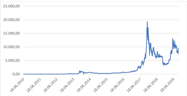
2016 was an important year for cryptocurrencies. We witnessed the Ethereum platform challenging Bitcoin in this year. To facilitate blockchain-based smart contracts and applications, Ether was used. With the help of Ether blockchain there were too many Initial Coin Offerings (ICOs) existed. Many of these blamed to be a scam or Ponzi scheme. As can be seen from Figure 1, next year Bitcoin reach its historical high with almost 20,000$ and currently in 2019 price of a Bitcoin is about 7,500$.
Figure 1. Daily price evolution of Bitcoin
Source: https://coinmarketcap.com/ 0,00 5.000,00 10.000,00 15.000,00 20.000,00 25.000,00
6
CHAPTER 3 LITERATURE REVIEW
In this section of the study, Bitcoin is investigated in three different ways. First of all, we discuss whether Bitcoin can be accepted as a currency. Secondly, we collected reviews on whether Bitcoin meets the efficient market hypothesis as an asset. Lastly, we searched for literature on the use of Bitcoin as a hedging instrument against both its price volatility and other investment instruments. 3.1. Evaluating Bitcoin as a Currency
Money, referred to as currency recognized as a medium of exchange for transaction purposes. It provides a reduction in transaction costs. In order to be useful, a currency should be;
• Fungible • Durable • Portable • Recognizable • Stable
As mentioned above, money’s main function is a medium of exchange. However, it has also secondary functions listed below.
• Unit of Account is one of the most important characteristics of the money. It means something that can be used to value goods and services, record debt and make the calculation. In another word, it is a measurement of value. The unit of account also has three main characteristics. Those are being;
➢ Divisible ➢ Fungible ➢ Countable
• Store of Value is another important characteristic of the money. Simply under no inflation assumption, putting money in a bank or a strongbox, and
7
take it out later, does not change the value. This property is useful for future savings.
• Standard of Deferred Payment, basically it is anytime that people receive something but only pay for it later, and the most common form of this is debt. With the “legal tender” term banks and institutions credit people or other institutions with the determined type of money for a while. For example, for the mortgage, people borrow from banks in any kind of money with a legal obligation, that is they have to repay their debt.
After giving classical properties of the currency, in this part, it is evaluated whether Bitcoin meets those properties will be discussed.
There is an ongoing discussion about whether Bitcoin is primarily an alternative currency or just a speculative asset (European Central Bank, 2012). In order to determine the values of currency, several theoretical models have been established like Interest Rate Arbitrage, Interest Rate Parity, etc. However, Bitcoin price is determined by users who exchange it on different markets. Because of the limited supply of Bitcoin, an increase in the number of Bitcoin participants is related to the price increase.
In order to evaluate the basic properties of the money for Bitcoin, starting with the medium of exchange. Bitcoin has no intrinsic value and worth of money depending on its usefulness for the consumer. Although the increasing number of merchants who accept Bitcoin as a payment method like Overstack.com, the Bitcoin market gap for the daily exchange is not worthy. Lielacher (2019) claims that the total number of Bitcoin wallets is 32 million. Furthermore, 2.3 million people used Bitcoin to make the payment from its first introduction until August 2018. Compared with the world population, which is about 7 billion, the total number of usages for the purchasing product or service appears extraordinarily negligible. In 2014, Bitcoin’s daily usage for the purchasing good and services is like 15,000 (Yermack, 2015) Furthermore, according to Coinbase co-founder Fred Ehrsam which is the most popular and used Bitcoin market, there were 24,000 merchants
8
are registered Coinbase. In brief, the Bitcoin market is a shallow and merchant number who accept Bitcoin as a medium of exchange scarce.
Another drawback for Bitcoin arises from the supply of it. Unless a consumer is a miner of Bitcoin, he or she must get it from an online exchange and then need to store it safely. Except for major exchange, liquidity is insufficient, and many exchange markets do not accept credit cards or other payment methods. Besides, bid-ask spread is also high.
Another obstacle can be said that for many consumers making their transactions with a credit card which allows postponing their repayments with zero cost for one month. Bitcoin-based credit card doesn’t exist yet and this option is not available. Lastly, transferring Bitcoin from one wallet to another requires a verification process, which takes on average 10 to 20 minutes. This delay is caused by the mining process. Many merchants and customers in today's standards vulnerable to wait this time lag.
Another feature of the money is being a unit of account. To measure goods and services in terms of Bitcoin, the price level should be stable in time. However, compared to other currencies Bitcoin price change is too volatile. Retailers who accept Bitcoin as a currency need to re-calculate price levels on a daily base which is costly for them and confusing processes for the consumers.
Bitcoin divided into 100 million Satoshi, and the price level for the merchants and the consumer is not calculated in a traditional way. Prices are in the right digit and the length of the decimal is long tailored. This results in making hard to compute price level of the good for costumer and according to Thomas et al. (2009), many people even well-educated would fail to reach calculation of the prices in terms of Bitcoin
The last property of the currency is the store of value. Throughout history, people tend to store their currency to spend in the near future. In order to protect their currency against theft, people put their money into Bank accounts which guarantee and insure against the theft. For Bitcoin, there are no options like Banks or legal
9
protection. Bitcoin can be stored either in exchange markets’ “digital wallets” or “cold storage”. However, storing in the market exchange wallet might be too risky because in the short history of Bitcoin there have been several failures of the exchange markets like Mt. Gox. Cold storage is another option for storing but costs are high compared to the traditional Bank services. Even if there were an option to store Bitcoin safe and cheap, people face managing volatility risk in the long run. For example, if anyone bought Bitcoin in December 2017, for today, there is at least a 50% percent decline in the price. Because of the exchange rate of the Bitcoin is too volatile and holding Bitcoin is quite risky, this undermines the ability of Bitcoin as a unit of account.
To sum up, being disconnected from the banking and payment system, decentralized structure (not issued by any state), not protected by legal authority, limited supply and high volatility make it hard to accept as a currency in a short time. Moreover, Bitcoin is not accepted as currency in China that announced to prohibit the use of Bitcoin as a currency for financial institutions (Ruwitch and Sweeney, 2013).
3.2. Evaluating Bitcoin for the Efficient Market Hypothesis (EMH)
Before starting our assessment, basic information about the efficient market hypothesis will be given. As the basis for modern portfolio theory, the efficient market theory is the basis of financial decision making. The theory of effective markets, which continued to be accepted in the field of finance, was put forward by the Nobel Prize-winning economist Fama (1960). In the efficient market hypothesis, prices include and reflect all rational expectations and available information. The underlying logic that random walk of the all subsequent prices which reflect random relation of previous prices. Since all available information is immediately reflected in asset pricing, tomorrow's prices are independent of today's prices and will only reflect news and information about tomorrow. Therefore, both novice and expert investors with diversified portfolio products will receive comparable returns regardless of their different levels of expertise.
10
• Weak form: Investors cannot use past information to predict future returns. However, because of the weak form, investor’s returns could be higher than the market return average because the return series follows a random walk. • Semi-strong form: Some information is not readily available to the public. Technical or fundamental analysis is not working to get more return compared with the market average. That is past information is not working for analysis. Yet, investors can pass the market return average.
• Strong from: All the information is reflected in the current price and for the future returns investors cannot go beyond the market return because all the information about the price given.’
With the given information, because Bitcoin is a crawling baby for academic research, some articles are summarized for Bitcoin and EMH.
In order to show whether Bitcoin is a speculative commodity or a currency Urquhart (2016) claims that it should provide efficient market hypothesis rules (FAMA). Even if in many articles’ Bitcoin was initially discussed in terms of safety, ethical and legal aspects, recent literature has examined Bitcoin from an economic viewpoint. For the EMH, future prices should not be foreseeable and price should follow the random walk.
To test this assumption in his work, data which includes daily price of Bitcoin between 2010 and 2016 divided into two parts. Whole data (between 2010 and 2013) divided parts tested with 5 different econometric tests. These tests aimed to determine autocorrelations, unit roots, nonlinearity, and long-range dependence in Bitcoin returns. Results show that Bitcoin returns do not provide EMH rules and the market is inefficient. However, for the second part of the data R/S Hurt statistic indicate Bitcoin returns have a semi-strong form of the EMH. The result compared with the emerging market for showing the maturity effect on asset return and EMH relation. He is claiming that with the time market or asset getting older, assets return tends to behave more efficient.
• Urquhart's (2016) study has influenced many people and it brings a new perspective for Bitcoin and EMH relations. After him, many articles were
11
written by different academicians like Nadarajah and Chu (2016). In their article, they specify EMH as “returns of a financial asset follow a stochastic process memoryless with the given information”. In this article the same data period was chosen to test Urquhart’s results. However, in their work, instead of using Bitcoin daily returns to test EMH efficiency, they used odd integer power of Bitcoin returns. Their claim powering of the returns does not influence any information loss. They extend Urquhart's works with more tests (8 different) and results show that the Bitcoin returns with calculated odd integer power fail to reject for many tests. Their results show that Bitcoin market is not as inefficient as Urquhart claims.
• For now, all research for Bitcoin and EMH tested for Bitcoin’s dollar price. Kristoufek (2018) extend this works with both dollar and yuan markets. Also, in this study, there is a new method namely Efficiency Index (EI) which calculated by Kristoufenk and Vosvrda in order to combine fractional dimension, entropy and long-time dependency. For the two different markets (USD and Yuan) Efficiency Index calculated and results show that distance to the efficient market situation. In this article, after a sharp increase or decrease period in Bitcoin price like the second half of 2016, the Bitcoin market seems efficient according to the efficiency index. This is explained with market volume and price fluctuation. It is claimed that with the regulations and big corporate player entrance and deepening the market volume would change current inefficiency.
• Another article to testing EMH for Bitcoin returns written by Bariviera (2017). In that article, it is claimed that Bitcoin cannot be a hedging instrument because of nonlinearities in the return-volume relationship for predicting returns. Different from Urquhart’s article, in order to test EMH, long memory of the time series tested with Hurst (1951) and extended version of Mandelbrot and Wallis (1968) findings to assess efficiency throughout time. This is also helping to determine the volatility of the daily returns for long-range memory. DFA results show to the necessity to divide data into two subsegments. The results of tests show that the second part of
12
the data can be evaluated compatible with EMH assumptions and the trend goes toward efficiency.
• Bitcoin price efficiency reconsidered in terms of long-range dependence and time variation in Tiwari et al. (2017) study. Efficiency index reconstructed with the long-time dependency and time variation perspective. The article suggests that under the different assumption and for an exceptional time period BTC market is efficient
• In order to investigate the existence of long-term dependence in the Bitcoin market and gap Katsiampa (2017) introduced the time-varying inefficiency of Bitcoin. The study shows long-term memory analyzed with R/S and variance ratio test. With the help of a rolling window approach determining in long term memory in Bitcoin to test dynamic efficiency of it, market return series presents an inefficient. Different from Urquhart’s or other results, dividing data into different samples does not help to make the market efficient.
To sum up, EMH for Bitcoin returns is a new and hot topic for many researchers. Many of them claim in current market prices Bitcoin behave weak or semi-strong efficiency. In addition, with the increasing number of participant and volume, for the recent time period Bitcoin seem more efficient. In the near future, with the help of more individual and corporate participants, accepted as a medium of exchange and widening derivates Bitcoin returns could be more efficient.
3.3. Bitcoin as a Commodity and Hedging Instrument
In order to evaluate an asset for fitting financial property to invest, it should be that we can count, liquidity, correlation with other assets and hedge capability. In recent years, Bitcoin and other cryptocurrencies have been evaluated within asset classes, such as stock and bonds. However, its popularity is mainly due to high volatility and exponentially increasing price and market volume. This dramatic increase in price attracts not only individual investors but also Wall Street banks and high-frequency traders. For example, with the peak level of Bitcoin price at the end of
13
2017, Chicago Board Options Exchange and Chicago Mercantile Exchange started to trading Bitcoin futures.
Bitcoin volatility is quite high, which has been addressed by many research like Bariviera (2017), Blau (2017), Katsiampa (2017), Gkillas and Katsiampa (2018). To eliminate loss caused by volatility, Bitcoin futures are investigated in Sebastiano et al. (2019) research. To show whether Bitcoin futures are a good hedge option or not GARCH model was used in their study. Results show that Bitcoin futures are an effective hedging tool at least a daily horizon.
Furthermore, there are several studies about Bitcoin and different stock markets return correlation. Dyhrberg (2016) indicates that Bitcoin is not uncorrelated with the assets in Financial Times Stock Exchange Index (FTSE) on average. Daily return of Bitcoin is not affected by changes in FTSE assets which creates an opportunity for investors to hedge some of the market risks. Yet, for Zhang et al. (2018) claims Bitcoin price changes are related to the economic fundamentals and market conditions. Vasilis et al. (2017) research supporting this by saying Bitcoin and asset prices are correlated in a shorter span.
Estrada (2017) shows the relation between Bitcoin price volatility and S&P 500. The study extended with realized volatility in Bitcoin and S&P 500 Volatility Index (VIX). Vector autoregressive models used in the study to proof writer assumptions. In order to test the relationship and correlation of the variables, Granger- causality test is used. Writer results show that volatility in Bitcoin Granger-causes S&P 500 series at 5% significance level. For the VIX, granger-causality exists in two directions. That is the reciprocal effect which is both Bitcoin price volatility and VIX changes affect another.
Bouri et al. (2017) extent assumption with testing whether Bitcoin is a hedging instrument for different assets and commodities like stocks, gold, oil and Us dollar index. The main argument in this study to see whether Bitcoin behaves as a diversifier. In this study, the bivariate DCC model is used to test authors' assumptions with daily and weekly time series. Results show that Bitcoin can be a good diversifier for Japanese and Asian Pacific stocks under adverse movement,
14
however, for S&P 500 and other stocks it has no diversifier feature.
To sum up, Bitcoin can be classified as an asset. As much research states that Bitcoin can be hedged with its future, it is a liquid and positive or negative correlation with other commodities or assets.
15 CHAPTER 4
RESEARCH DESIGN AND METHODOLOGY
This chapter of the study focuses on the research methodology. The sample selection and data collection processes are described; variables of the study and their operationalization are introduced, and data analysis methods are explained. 4.1. Data Collection Method
For this research, Google Trends search (GTS) data are used. Data are gathered from https://trends.google.com and it shows the relative popularity for “Bitcoin” keyword. This website does not provide exact search volumes, but it provides scaled trends for a keyword in a specified date range for selected variables.
As Google Trends explained as in “https://ahrefs.com/blog/how-to-use-google-trends-for-keyword-research”, data show the popularity ratio of Bitcoin to all other possible searches and it is scaled on a range of 0 to 100 for each different query. For this study, the daily date obtained for the period from January 2017 to September 2019. In order to overcome Google’s limitation on a query for a long time period, the last 3 years’ data gathered from 4 different windows which have the same time interval. In order to re-scale and obtain daily trend data, the whole sample gathered weekly, and weekly data readjusted and converted into daily data with 4 different time windows. In summary; the following steps are constructed to build daily scaled trends data for 3 years:
1. Weekly Bitcoin trends data are collected from Google Trends.
2. Daily Bitcoin trends data are fetched from Google as 4 parts because of limitations.
3. To use 4 different parts as 1-part, daily coefficients are used to convert weekly trends data to daily data.
Google Trends gives you the freedom to choose keyword search results by country, city, or worldwide. In our study, the data are gathered for worldwide and 20 selected countries. These countries were chosen in accordance with their rank on worldwide search. For the first 15 countries, selection criteria are determined with their rank
16
in worldwide results. Remaining 5 countries selected by their population size. That is to say, except for the first 15 countries, the most populous countries are selected. In order to normalize the scaled data, all values are compressed between 0 and 1 according to maximum and minimum values. By multiplying the compressed results by 100, we have achieved the final Google Trends results worldwide and by country. The whole process for normalization of the data is made in SAS Enterprise Miner and SAS Enterprise Guide. In this part, to normalize our data “PROC STDIZE” procedure is used.
Normalization method used as a given equation;
𝑍
𝑖=
𝑥𝑖−𝑚𝑖𝑛(𝑥)𝑚𝑎𝑥(𝑥)−𝑚𝑖𝑛(𝑥)
(1)
Sample of the data includes daily data of Bitcoin in terms of USD rate (XBTUSD) which provides the price levels that are robust in our research. Data sample time period from January 2017 to September 2019. The time span of the data covers market stress events that exist in Bitcoin prices as can be seen in Figure 2. We obtain
the transaction data via the web-based Bitcoin data
provider https://coinmarketcap.com which provides up-to-the-minute updates for all the market data. Our dataset comprises High, Low and Closed prices as well as exchange volumes in BTC a daily basis. In this study, the daily prices of Bitcoin were determined in accordance with Google Trends dates which started from January 2017 to September 2019.
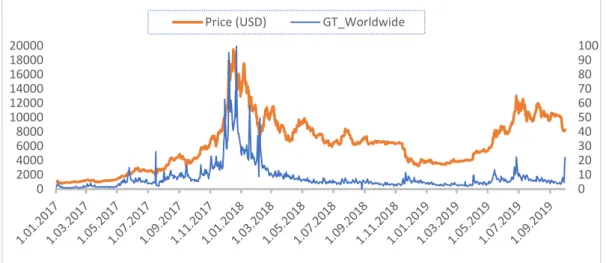
Figure 2. Bitcoin price and scaled Google Trends worldwide result for Bitcoin search between January 2017 to September 2019.
17
Figure 2. Bitcoin price and scaled Google Trends worldwide result for Bitcoin search between January 1𝑠𝑡 2017 to September 30𝑠𝑡 2019
4.2. Descriptive Statistics
Data analysis of this study was made by using SAS Enterprise Miner and SAS Enterprise Guide.
Normalized GTS data and Bitcoin prices were combined to create the final data. Our final data includes 1003-day Google Trends information for worldwide and selected 20 countries as well as Bitcoin closing price, daily lowest and highest level. Firstly, descriptive statistics for Bitcoin prices are listed below:
Table 1. Descriptive Statistics Results
N=1003 Descriptive Statistics Results
Mean 6169.07 Std Dev 3645.62 Minimum 777.76 Maximum 19497.4 Mode 1179.97 Median 6297.57 Range* 18719.64 5th Pctl** 1042.9 95th Pctl** 11941.97
* This is the difference of highest and lowest price ** This is the lowest 5% threshold level
*** This is the highest 95% threshold level
0 10 20 30 40 50 60 70 80 90 100 0 2000 4000 6000 8000 10000 12000 14000 16000 18000 20000
18
Table 1 shows that the average price of Bitcoin is around 6,150$ and standard deviation is around 3600$. Moreover, the table shows the minimum and maximum price of Bitcoin as well as the difference of them namely “Range” which our scaling procedure depends on.
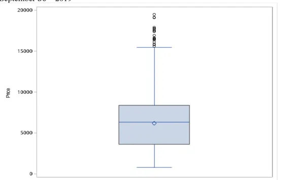
In our data, we don’t have any missing variable problem. However, as can be seen from the table, there is an outlier effect on our data and Bitcoin price is not distributed normally. In order to observe outliers, box plot is drawn which displays the range, interquartile range and mean of a variable. Krzywinski et al.(2014) claim that using box plots in the analysis to observer outliers is too useful because it characterizes a sample using the 25th, 50th and 75th percentiles and the interquartile range, which covers the central 50% of the data.
Like descriptive statistics, Figure 3 represents a Box-and-whiskers plot which shows the interquartile range which is between 3,000$ and 8,000$ and the mean is around 6,000$. However, there are some extreme values for the closing price which is higher than 15,000$. For some studies, extreme variables can be evaluated as outliers and they might be removed from data, yet, these variables were not excluded in our study because they are meant for the study.
Figure 3. Box-and-whiskers Plot for Bitcoin price time between January 1𝑠𝑡 2017 to September 30𝑠𝑡 2019
19
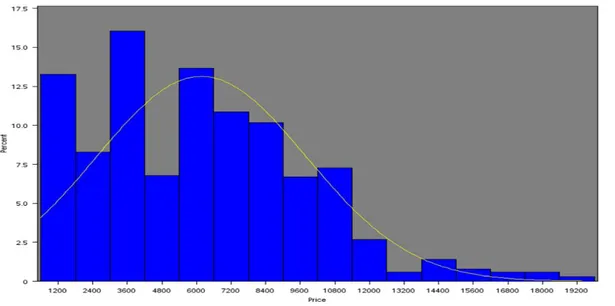
In the next step, the histogram is drawn for Bitcoins’ closing price. Additionally, some statistical results are calculated such as the mean, median, skewness and kurtosis to show that our data are not normally distributed.
As can be seen from Figure 4, the histogram of Bitcoin price is right-skewed which is also called positive-skew distribution. That’s because there is a long tail in the positive direction on the horizontal axis.
Figure 4. Bitcoin Price Histogram
Furthermore, moments results reported in table 2, shows the skewness ratio is between 0.5 and 1 which means that our distribution is moderately skewed. The mean of the Bitcoin price is also at peak at the right side of the graph.
Table 2. Moments Results for Figure 4
In order to standardize the distribution of Bitcoin price, we tried many transformation methods discussed in Hosseinifard et al. (2009), namely lognormal, power, and square root which is often used in both applied and theoretical statistics.
Moments
N 1003 Sum Weights 1003
Mean 616.906.777 Sum Observations 6187574.97 Std Deviation 36.456.178 Variance 13290529.2 Skewness 0.64621303 Kurtosis 0.31960195
20
Yet, for all different standardization methods, our distribution is not standardized. So, we decided to continue with non-normal data in our analysis.
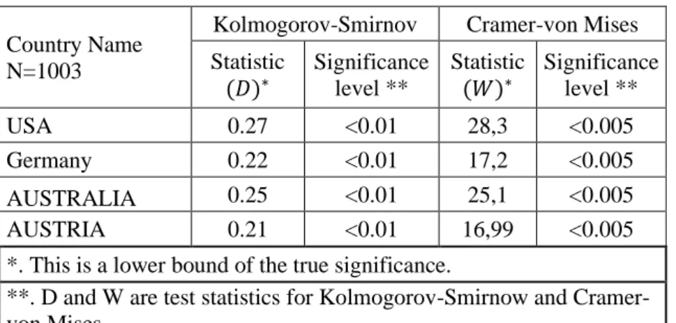
Furthermore, for the selected 20 different countries and worldwide Google Trends search query results tested. As the Bitcoin price, scaled GTS queries for all countries are right-skewed and non-standardized distribution they have. Table 3 shows some selected countries to show the unstandardized distribution of GTS queries.
Table 3. Normality Test Results Sampled Countries Country Name
N=1003
Kolmogorov-Smirnov Cramer-von Mises Statistic (𝐷)∗ Significance level ** Statistic (𝑊)∗ Significance level ** USA 0.27 <0.01 28,3 <0.005 Germany 0.22 <0.01 17,2 <0.005 AUSTRALIA 0.25 <0.01 25,1 <0.005 AUSTRIA 0.21 <0.01 16,99 <0.005
*. This is a lower bound of the true significance.
**. D and W are test statistics for Kolmogorov-Smirnow and Cramer-von Mises
As it is mentioned before, the normalization method is applied for not only Google Trends query results but also Bitcoin price data. Figure 2 shows that the outliers for both Google Trends searches and Bitcoin price points overlap at a similar time period. Since extreme values are observed in the same periods and this match is significant in correlation analysis, we continue with non-standardized data.
4.3. Correlation Analysis of Bitcoin Price and Google Trends Queries
In this part, GTS data and Bitcoin price correlation will be examined. In general, the outlier is expected to disrupt the correlation analysis but, in our data, as can be seen from Figure 2, outliers of both series exist in a similar time period. Furthermore, selected countries’ trend searches are also evaluated. According to the results, as we mentioned before, all countries and worldwide GTS have a right-skewed distribution. Moreover, for all normalized and scaled searches which are between 0 and 100, 99% of data have a lower than “60 scaled value” trend for all countries. This result shows that the outlier effect is similar to the country level.
21
In this step, correlation analyses are conducted for each country search and the worldwide search as well as Bitcoin price. Initially, to check the correlation between price and GTS we used Pearson correlation.
The Pearson product-moment correlation measures both the strength and the direction of a linear relationship. If the first variable is an exact linear function of the second variable, it shows that a relationship exists between these variables. According to the correlation coefficient sign which gives the direction of the correlation, it is decided whether there is a negative or positive correlation between these variables.
The formula for the population Pearson product-moment correlation, denoted 𝜌𝑥𝑦
is;
𝜌
𝑥𝑦=
𝐶𝑂𝑉(𝑥,𝑦) √𝑉(𝑥)𝑉(𝑦)=
𝐸((𝑥−𝐸(𝑥))(𝑦−𝐸(𝑦))
√𝐸(𝑥−𝐸(𝑥))2𝐸(𝑦−𝐸(𝑦))2
(2)
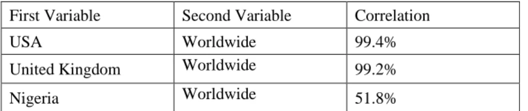
Table 4 given below, shows the correlation between the worldwide and country- level search examples.
Table 4. GTS and Selected Countries Pearson Correlation
First Variable Second Variable Correlation
USA Worldwide 99.4%
United Kingdom Worldwide 99.2%
Nigeria Worldwide 51.8%
It shows that some countries like the USA or the United Kingdom are highly correlated with worldwide, whereas some countries like Nigeria have low correlation. This means that the popularity of Bitcoin for the USA and the United Kingdom appears similar whereas Nigeria GTS behaves differently within the given time period. In our study, we assume that down to %70 correlation, can be enough to accept it as a high correlation. Schober et al. (2018) claim that more than %70 correlation can be classified as a "strong correlation" which supports our threshold level in our study.
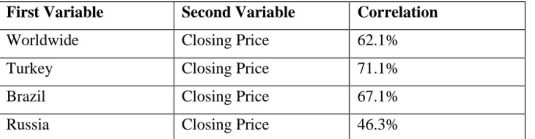
Furthermore, we checked the correlation between GTS and Bitcoin price. Table 5 shows the correlation between the Bitcoin closing price and Google Trends searches
22
of countries on a daily base. The most correlated country in our data is Turkey and the least correlated one is Russia. Therefore, correlation with closing price significantly changes for each country level.
Table 5. GTS and BP Pearson Correlation
First Variable Second Variable Correlation
Worldwide Closing Price 62.1%
Turkey Closing Price 71.1%
Brazil Closing Price 67.1%
Russia Closing Price 46.3%
According to some studies like Myers et al (2006) and Chok (2010) Pearson’s correlation works in data that have a normal distribution. Myers et al. (2006) study it is claimed that for Pearson correlation, data should have the standard normal distribution. If data are not normally distributed, then Spearman’s rank-correlation coefficient should be used in the analysis. As we mentioned before, our Bitcoin price data is not normally distributed. Therefore, we calculate the correlation with Spearman’s rank-correlation in order to calculate the correlation of variables more accurately. Spearman’s rank-correlation is a non - parametric measurement of association that is based on the rank of the data values. The correlation range in Spearman is the same as with the Pearson which is from -1 to 1. Unlike Pearson’s correlation, Spearman correlation is robust to outliers and it does not expect that the data are normal. It applies to the rank and provides a measure of the monotonic relationship between given variables. Spearman’s correlation formula is given below.
θ=
∑ ((𝑹𝒊 𝒊− 𝑹̅)(𝑺𝒊−𝑺̅)) √∑ (𝑹𝒊 𝒊−𝑹̅)𝟐∑ (𝑺𝒊 𝒊−𝑺̅)𝟐(3)
In this formula 𝑹𝒊 is the rank of one variable, 𝑺𝒊 is the rank of another variable, R is the mean of the 𝑹𝒊 values, and S is the mean of the 𝑺𝒊 values.
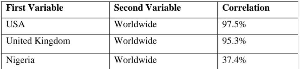
Table 6 represents Spearman’s correlation of sampled country's searches between worldwide searches.
23
Table 6. GTS and Sampled Countries Spearman Correlation
First Variable Second Variable Correlation
USA Worldwide 97.5%
United Kingdom Worldwide 95.3%
Nigeria Worldwide 37.4%
Compared with Pearson’s results, the USA and the United Kingdom are still the highest correlated countries with worldwide, and Nigeria is the lowest one. However, for both correlated and uncorrelated countries, their correlation level is decreased. Nigeria is a good example to show Pearson’s and Spearman’s correlation difference which drops from 52 to 37.
Table 7 represents the Spearman’s correlation of closing price and sampled countries. In this table, different than the countries and worldwide correlation, Spearman’s correlation shows bettering relationship for worldwide and price, whereas Brazil and Russia’s correlation between closing price worsening.
Table 7. GTS and BP Spearman Correlation
First Variable Second Variable Correlation
Worldwide Closing Price 64.7%
Turkey Closing Price 79.7%
Brazil Closing Price 64.3%
Russia Closing Price 34.0%
Japan Closing Price 27.0%
After all, we observe some countries GTS is highly correlated with worldwide GTS some are not. Furthermore, Bitcoin’s daily closing price level correlated with worldwide GTS (around 65%) and some selected countries’ GTS. However, correlation does not imply causality. Since, in some cases, an underlying causal relationship might not exist According to Bianchi (1995), correlation itself can provide misleading inference about the underlying relationship of causality. In order to test the high correlation and causality, the Granger Causality test will be performed in the following parts.
24 4.4. Clustering Countries
In the previous chapter, we explain that most of the countries are highly correlated with worldwide and each other. Therefore, in this part variable clustering method is used to cluster these similar countries.
The variable clustering feature is used for data reduction and it selects the best variables which represent all other variables in the same cluster. In order to select different behaviors for selected countries in our data, we used this methodology and we grouped 20 countries in 5 different clusters. SAS Enterprise Miner “Varibale Cluster Node” is used for grouping the countries in terms of their scaled Google Search time series. This process is summarized below.
Variable Clustering node takes all data as one single cluster. Then it follows the below steps:
1) Clustering Variable Node chooses a cluster for splitting. This cluster might have the smallest variation or have the highest eigen value.
2) Chosen cluster is split into two clusters and 2 principal components are selected as the best variables.
3) It assigns all the other variables into these two clusters according to their higher correlation.
4) Each variable re-assigned to a cluster again to maximize the variables. 5) It stops when each cluster has one eigenvalue which is greater than 1. In our study, correlation is used to cluster 20 countries and worldwide Google Search series together. Additionally, we detected principal components which are the best representation variables for our clusters. The best variable in each cluster is the variable that has the highest R2 Ratio.
The following dendrogram plot shows cluster organization and clusters which are determined with their variance. Figure 5 shows the dendrogram plot, 5 cluster is enough to keep distances sufficiently.
25 Figure 5. Selected Countries Dendrogram
After 5 clusters are chosen, countries Google Trends data is clustered according to their correlation and Figure 6 shows the center and nearness of clusters for each country as below.
26
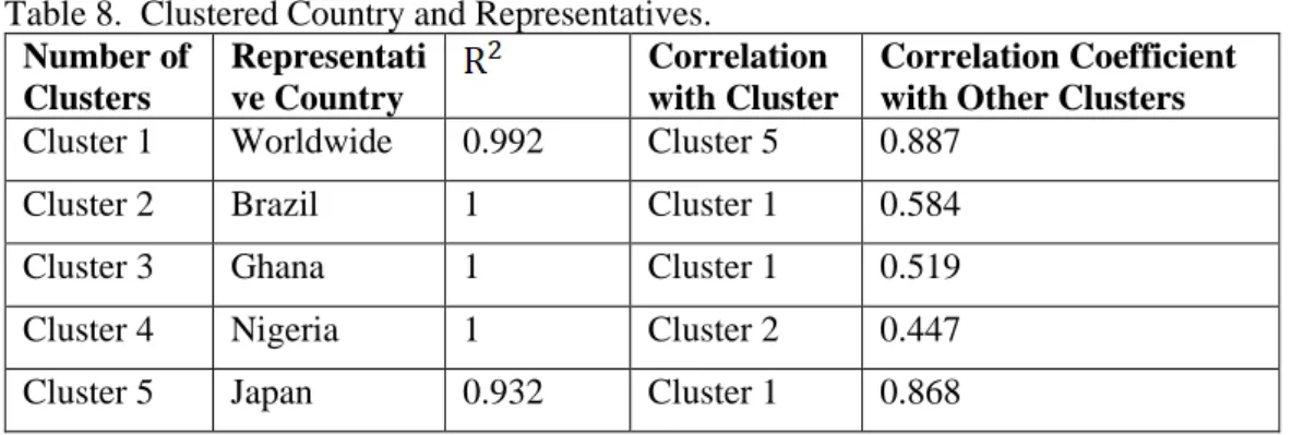
The first cluster contains 15 countries and worldwide, which represents these countries with 0.88 , which is in the center of the first cluster. Brazil, Ghana, and Nigeria are represented in 3 different clusters. This is because the Google Trends searches queries of these countries do not any relation with the data from other countries.
For the last cluster, it contains 3 countries which are Japan, China and South Korea. Japan is the representative country for this cluster.
The table shows the representative countries for each cluster and their representative power in those clusters.
Table 8. Clustered Country and Representatives. Number of Clusters Representati ve Country Correlation with Cluster Correlation Coefficient with Other Clusters Cluster 1 Worldwide 0.992 Cluster 5 0.887
Cluster 2 Brazil 1 Cluster 1 0.584
Cluster 3 Ghana 1 Cluster 1 0.519
Cluster 4 Nigeria 1 Cluster 2 0.447
Cluster 5 Japan 0.932 Cluster 1 0.868 4.5. Defining Break Point
As can be seen from Figure 2, the correlation between GTS queries for worldwide and Bitcoin price corrupt somewhere. In order to determine the breaking point, the following analysis is made.
In this analysis scaled closed price and scaled worldwide trend data is used. The goal is to find the farthest point between closing prices and the Google search data. For each day in our data, the difference between these 2 variables was calculated as in the following formula.
Diff=abs(Closing_Price – Worldwide) (4)
Then the maximum point was selected as the breakpoint. Figure 7 shows the differences between the closing price and worldwide searches.
27 Figure 7. The Difference between GTS and BP
Since, the maximum difference appears on the 6th of January 2018, this point is
selected as the breaking point. After deciding on the break point, the whole working data is divided into two parts. The data before 6 January 2018 are determined as 1st part and the data after this date are determined as 2nd part. Subsequent analysis was performed with these parts instead of all data.
4.6. Crating New Variables
In this section, in order to test Granger-causality in the following section, we are creating new variables with gathered data from https://coinmarketcap.com. Data includes “daily low” and “daily high” variables, which are the lowest and highest price levels in a day. With the help of these variables, two new variables were calculated.
These are:
• Daily Volatility: It shows the percentage of the difference between daily high and low price.
28 Volatility= 𝐷𝑎𝑖𝑙𝑦_𝐻𝑖𝑔ℎ – 𝐷𝑎𝑖𝑙𝑦_𝐿𝑜𝑤
𝐷𝑎𝑖𝑙𝑦_𝐿𝑜𝑤 *100 (5)
• Daily Change in Price: It shows the daily change in the closing price in terms of the previous day.
Δ Price=𝑃𝑟𝑖𝑐𝑒𝑡 – 𝑃𝑟𝑖𝑐𝑒𝑡−1
𝑃𝑟𝑖𝑐𝑒𝑡−1 *100 (6)
Firstly, worldwide GTS queries and these two new created variables’ correlation have been calculated for the whole time period. Spearman correlation method is used for these analyses and the correlation coefficient for volatility and change in price are 0.64 and 0.006 respectively. These correlation ratios show that worldwide searches and daily volatility has a statistically significant relationship because their correlation is around %64. However, for daily change in price (Δ Price) correlation coefficient is close to “0” which means there is no significant relationship between worldwide searches and Δ Price. For the following test, the daily change in price variable is not used anymore. However, 64% correlation is meaningful to test our hypothesis for the following sections.
Daily volatility, for each part of our study data which divided into 2 parts at the previous section, is subjected to correlation analysis. In addition, correlation coefficients were calculated for 4 representative countries and worldwide because in the previous section, 20 countries clustered together in 5 different groups with the clustering method.
For the first part which is between 01 January 2017 and 06 January 2018 results listed below.
Table 9. First Part Spearman Correlation Spearman Correlation Coefficients, N = 371
Variables Name Worldwide Brazil Ghana Nigeria Japan
Closing Price 0.93185 0.86243 0.69514 0.2376 0.8253
Daily Volatility 0.58245 0.5361 0.38933 0.27522 0.57184
When the results compared with the whole data correlation coefficient, the daily volatility coefficient has decreased from 64% to 58% for the first part of the data.
29
Therefore, it is expected that this variable has a stronger relationship in the second part.
Table 9 shows 5 different clusters of Google Trends series and their correlation between daily volatility and closing price. The highest correlated cluster is worldwide and the lowest one is Nigeria and their correlation coefficients are 58% and 27% respectively.
Table 10 shows the correlation results for the second part of the data which includes all the variables between the January 6, 2018, and September 30, 2019 time interval.
Table 10 Second Part Spearman Correlation Spearman Correlation Coefficients, N = 371
Variables Name Worldwide Brazil Ghana Nigeria Japan
Closing Price 0.77807 0.52432 0.27593 0.33846 0.56464
Daily Volatility 0.67049 0.64942 0.36818 0.53136 0.39846 It is clear that for the second part of the data, daily volatility and worldwide search correlation coefficient jump to 78%. On the other hand, closing price and worldwide search correlation have decreased from 93% to 67% which means a strong correlation between the closing price and worldwide search is rejected in this part.
Moreover, when the correlation coefficients of 5 different clusters are examined for each part, the following results are obtained.
➢ We have stated that the clusters created by Brazil, Ghana, and Nigeria contain only these countries’ data. When these 3 different clusters are compared with the first cluster which contains 15 different countries and represented by the worldwide, very different behaviors are observed in terms of correlation analysis. For example, in all analyzes, it was found that the correlation coefficients of these clusters for all variables were much lower than the first clusters, and sometimes they had a meaningless relationship for the variables.
30
➢ As we said before, for the second part the data Google Trend search scaled variables are more correlated with daily volatility, instead of the closing price. However, this can be said only for the first cluster represented by worldwide. For the rest of the clusters which consist of only 5 countries, this situation is working in the opposite direction. That is, for the remaining four clusters, Google Trend search variable is somehow uncorrelated with the closing price and daily volatility or correlated just for the closing price. These differences can be observed not only for the whole data but also in 2 different parts where the data is divided.
4.7. Prediction Analysis
In this part, we wanted to test whether daily fluctuations in Bitcoin price and Google Trend searches are in the same direction. In order to test this assumption, we created two new binary variables. These are:
Change in Price (CP): Difference between the current price and the previous day price. If the result is negative then the flag is 0, and if vice versa then the flag is 1. CP=Pricet – Pricet−1
Code used in SAS Enterprise Miner: if CP > 0 then 1 else 0
Change in Search (CS): Difference between Google Trend search and previous day Google Trend search. If the result is negative then the flag is 0, and if vice versa then the flag is 1.
CS=Searcht – Searcht−1
Code used in SAS Enterprise Miner: if CS > 0 then 1 else 0
These flags assigned to both Bitcoin price and each countries’ Google Trends search queries variable for all dates. After that, these flags have been summed up for each country and confusion matrix is created.
Confusion matrix which is also known as error matrix shows precision, accuracy and misclassification rates. This is supervised learning and it is used to measure the performance.
31
In order to understand the calculation method easily, the sample table for flags and accuracy and misclassification calculation methods are summarized below.
Table 11 Confusion Matrix Explanation
Δ CP Flag Δ Change in Search flag Explanation
0 0 False Positives (FP) 0 1 False Negatives (PN) 1 0 True Negatives (TN) 1 1 True Positives (TP) Accuracy: (TP + TN) / (TP+TN+FP+FN) Misclassification: (FP + FN) / (TP+TN+FP+FN)
Furthermore, in order to interpret the confusion matrix, Matthews correlation coefficient (MCC) is used. MCC is simply a correlation coefficient between observed and predicted binary variable and it returns between -1 and +1. 1 means perfect prediction and -1 means total disagreement. MCC formula is given below.
𝑀𝐶𝐶 =
(𝑇𝑃𝑥𝑇𝑁)−(𝐹𝑃𝑥𝐹𝑁)√(𝑇𝑃+𝐹𝑃)(𝑇𝑃+𝐹𝑁)(𝑇𝑁+𝐹𝑃)(𝑇𝑁+𝐹𝑁) (7)
Confusion matrix and MCC are calculated for 5 different clusters for whole data. Table 12 indicates the accuracy and the MCC ratios.
The table shows that the accuracy rates and misclassification rates are similar for 5 cluster countries. It means that these dummy variables which can be evaluated as flags did not provide differentiation between clusters. Furthermore, MCC values for all clusters are too close to 0 which means Bitcoin price change cannot be predicted by daily change in Google Trend search variable. This study shows that the prediction of the Bitcoin price with the help of GTS without any
32 Table 12 Confusion Matrix and MCC Results
Clusters Δ CP flag
Δ CS
flag Count 1002 Accuracy MCC
Misclassification Rate Brazil 0 0 221 22% 48% 0.113 52% 0 1 222 22% 1 0 303 30% 1 1 256 26% Ghana 0 0 232 23% 51% 0.116 49% 0 1 211 21% 1 0 282 28% 1 1 277 28% Japan 0 0 213 21% 48% 0.115 52% 0 1 230 23% 1 0 294 29% 1 1 265 26% Nigeria 0 0 217 22% 47% 0.112 53% 0 1 226 23% 1 0 310 31% 1 1 249 25% Worldwide 0 0 271 27% 47% 0.106 53% 0 1 172 17% 1 0 355 35% 1 1 204 20%
The table shows that the accuracy rates and misclassification rates are similar for 5 cluster countries. It means that these dummy variables which can be evaluated as flags did not provide differentiation between clusters. Furthermore, MCC values for all clusters are too close to 0 which means Bitcoin price change cannot be predicted by daily change in Google Trend search variable. This study shows that the prediction of the Bitcoin price with the help of GTS without any transformation or lagged variable will not give meaningful results.
33 4.8. Stationary Tests of Variables
In the previous sections, it was detected that closing price and daily volatility is correlated with Google trend searches at first & second parts. However, this result does not guarantee that this variable can help forecasting Bitcoin price change by using Google searches. In this section, we tried to explain the causality of the results.
In order to determine the causality relationship and the direction of it, the Granger causality test can be used. As a prerequisite, working data must be stationary to apply the Granger-causality test because it is very sensitive to the choice of lag length and to the methods employed in dealing with any non-stationarity of the time series. The stationarity test is used to determine whether differencing is necessary. Most of the time series are non-stationary because of seasonality effects. Before applying Autoregressive Moving Average (ARMA) models to time series data must be transformed into stationary. Therefore, firstly stationary test was applied to identify whether data has seasonality or not. If the data is nonstationary, it requires differencing.
The Augmented Dickey-Fuller (ADF) test can be used to test three types of data generation models for stationary. These are;
• Zero-mean stationary (zero mean), • Nonzero-mean stationary (single mean), • Linear time trend stationary (trend).
When there is a unit root (that is, the series is nonstationary), the sum of the autoregressive parameters is 1 and hence beta=0. The ADF tests build on beta. There are three kinds of tests under the ADF tests: rho (p) test, tau (t) test, and F test. The rho test is the regression coefficient test, which is also called the normalized bias test. The tau test is the studentized test. The F test is a joint test for unit root. Table 13 presents the null hypotheses and decision rules for the three test statistics under the three different model types.
34 Table 13 Stationary Test Steps
Rho Test Tau Test F- TEST
Types 𝐻0 p-value 𝐻0 p-value 𝐻0 p-value
Zero mean δ =0 Stationary if
low δ=0
Stationary if
low N/A N/A
Single mean δ =0 Stationary if
low δ=0 Stationary if low δ =α0=0 Stationary if low Trend δ =0 Stationary if low δ=0 Stationary if low δ=ϒ=0 Stationary if low
In this table 𝛼0 is the vector intercept in the test regression fort the single-mean model,
∇𝑦𝑡=α0+ δ𝑦𝑡−1+𝜃1∇𝑦𝑡−1+… + 𝜃𝑝∇𝑦𝑡−𝑝+𝑒𝑡 (8)
And ϒ is the parameter of 𝑡 in the test regression fort the trend model, ∇𝑦𝑡=α0+ ϒ𝑡 + δ𝑦𝑡−1+𝜃1∇𝑦𝑡−1+… + 𝜃𝑝∇𝑦𝑡−𝑝+𝑒𝑡 (9)
As shown in the regression for the single-mean model, when δ=0 (that is there is a unit root), the intercept α0 = δµ=0. The F test with a joint hypothesis of zero intercepts and zero slopes can be used as a unit root test fort the single-mean model. The F test for the trend model follows a similar logic. When δ=0, ϒ = −δβ = 0 the F statistic for the trend model, therefore, tests the joint null hypothesis: δ= ϒ=0. When testing for unit root, the tau test is more powerful than F-test.
In order to do the stationary tests of the variable SAS Enterprise Miner ARIMA method is used.
Firstly, observation and correlation graphs were created by SAS Enterprise Miner before applying the augmented Dickey-Fuller (ADF) test. This is because we tried to understand whether our sample is stationary or not. While doing ADF tests that is necessary if the time series is non-stationary, it is essential to detect how many differences will be used and which model will be used. (zero mean, single mean, or trend).
35
The results of the graphical series correlation analysis taken from SAS Enterprise Miner are shown in Figure 8. It shows trend and correlation results for the first part which includes data for the time between 01 January 2017 and 06 January 2018. Before we started to, some explanations are listed below to give a brief description of the figure divided into 4 windows.
There are four graphs of the closing price. These graphs are: • The time series plot of the series
• The sample autocorrelation function plot (ACF)
• The sample inverse autocorrelation function plot (IACF) • The sample partial autocorrelation function plot (PACF)
These autocorrelation graph (ACF) shows the degree of correlation with historic variables that is called lag variables which is24 by default in SAS Enterprise Guide. Figure 8. Stationary Test Results Taken for First Part
It is obvious that the closing price of Bitcoin has time - trend mean is not closed to zero. As mentioned before it is a trend data, “Trend” type will be the most important
36
test for this part. In table 14, the row for “Lags” columns is zero means that AR(1) model was used for this test. Tau test statistics are mostly used to decide whether to reject the null hypothesis. P-values for Tau statistics are greater than 0.01, and the null hypothesis (the series is nonstationary; that is, there is a unit root) cannot be rejected at the 1% level.
For the first part of our data, Dickey-Fuller Unit Root (ADF) is applied with one lag results is shown in Table 14.
Table 14 ADF Test Result for First Part Dickey-Fuller Unit Root Tests
Type Lags Rho Pr <
Rho Tau Pr < Tau F Pr > F Zero Mean 0 3.4263 0.9995 2.54 0.9975 Single Mean 0 2.8975 0.9996 1.53 0.9994 3.3 0.2252 Trend 0 -1.4503 0.9816 -0.45 0.9855 2.53 0.6712 ADF Test Hypothesis
𝐻0: Stationary
𝐻𝑎: Non-Stationary
Based on the p-values of all tests, the null hypothesis is rejected at the 1% level. It is necessary to convert this data from non-stationary to stationary level. Therefore, difference (first- order integration) was calculated as Price(t) – Price(t-1) for first part of data. All process was done again with new transposed data. As can be seen in Figure 9 partial autocorrelation functions (PACFs) decreases dramatically after first- order integration and PACF plot and ACF do not increase as much as the lag increases in ACF plot. As a result, for the first part of our data, to make our series stationary, we checked Augmented Dickey-Fuller Unit Root (ADF) again and the result is shown in Table 15. This is because even if the first plot seems that there is no trend and the mean is around zero, so at first, for the Dickey-Fuller test, we need to check the zero mean. Furthermore, the graph does not give us information about single mean. To check stationary of Bitcoin price at first order integration as we said we do the second test.
37
Figure 9. Stationary Test After First-order Integration
Table 15 ADF Test with I(I) Results for First Part Dickey-Fuller Unit Root Tests
Type Lags Rho Pr < Rho Tau Pr < Tau F Pr > F
Zero Mean 0 -317.27 0.0001 -16.66 <.0001
Single Mean 0 -320.905 0.0001 -16.8 <.0001 141.18 0.001 Based on the p-values of both tests, the null hypothesis is rejected at the 1% level, indicating that the differenced time series for the first part of the data is being stationary.
All calculations are repeated for the second part of data which is between 06 January 2018 and 30 September 2019 in Figure 10.
It seems that the second part of the data has no time trend, but the mean of the Bitcoin price is not close to zero. Using first-order (I(1)) integration will be enough for the stationary because partial autocorrelation functions (PACFs) decreases dramatically after the first lag. Moreover, as can be seen in Figure 10, ACF does not increase when the lag increases in ACF plot. Therefore, first order integration is selected for the single mean stationary test. First order one lagged stationary test result listed below.