C om mun.Fac.Sci.U niv.A nk.Series A 1 Volum e 67, N umb er 1, Pages 198–210 (2018) D O I: 10.1501/C om mua1_ 0000000842 ISSN 1303–5991
http://com munications.science.ankara.edu.tr/index.php?series= A 1
STOCHASTIC STABILITY IN TERMS OF AN ASSOCIATED TRANSFER FUNCTION MATRIX FOR SOME HYBRID
SYSTEMS WITH MARKOVIAN SWITCHING
CHAFAI IMZEGOUAN
Abstract. This work is devoted to stability for a dynamical system with Markovian switched controller and a …nite number of linear di¤erential sub-systems. We suppose su¢ cient conditions on a state space representation of an associated transfer function matrix which guarantees stochastic stability. The given examples are detailed to illustrate the main result.
1. Introduction
Much attention has been drown by switched dynamical systems due to their extensive applications in many …elds such as economic systems, …nancial markets, communication networks..., (For more information see [4]). The important problem is to ensure stability because the typical problem of switched systems is as follow: it can be that all sub-systems of the jump system are stable but the switched system can be unstable [20].
We refer the reader to the book by Sun and Ge ([17]) for examples, and a recent systematic manner presentation of the stability theory of general switched systems under di¤erent switching mechanisms. The other new stability issues, concepts and methods for Markovian switching systems, were introduced by Benaîm et al. in [2] where the same system was studied supposing also that the matrices of the subsystems are Hurwitz (all eigenvalues with negative real parts) without supposing that the subsystems are in companion form. The authors have dealt with the stability problem, but only for planar randomly switched systems and they have proved that under some conditions on the Hurwitz matrices, the norm of the continuous component may go to zero or to in…nity depending on the existence of few or many jumps.
Received by the editors: December 05, 2016; Accepted: May 15, 2017. 2010 Mathematics Subject Classi…cation. 93E15, 60J27, 37M05.
Key words and phrases. Hybrid switching system, transfer matrix, Markov jump, companion form, stochastic stability, Lyapunov function, stationary distribution.
c 2 0 1 8 A n ka ra U n ive rsity C o m m u n ic a tio n s d e la Fa c u lté d e s S c ie n c e s d e l’U n ive rs ité d ’A n ka ra . S é rie s A 1 . M a th e m a t ic s a n d S t a tis t ic s .
Zhu et al. ([23]) have studied stability of random switching systems of di¤eren-tial equations. They have presented su¢ cient conditions in terms of a Lyapunov function and they also established veri…able conditions for stability and instability of systems arising in approximation. They have used a logarithm transformation to derive necessary and su¢ cient conditions for systems that are linear in the continu-ous state component. They have concluded their paper with several examples, and have noticed a somewhat di¤erent behavior from the well-known Hartman-Grobman theorem. A deterministic counterpart in R2 was detailed by Balde et al.[1] in the case of arbitrary switching. Also, an implemented method of simulation as Scilab and Matlab toolboxes was presented in [5] and [6] for the deterministic switching case.
In this paper, we consider a hybrid system modulated by a random-switching process which is equivalent to …nite number of ordinary di¤erential equations cou-pled by a switching or jump component. The hybrid system with Markovian switched controller is supposed associated with a transfer matrix G(s) with s a complex number. The motivation behind this quite new formulation is well de-scribed in the articles by Kouhi and al. ([11] and [12]). The main contribution in this paper consists on the use of the stochastic machinery in order to obtain some quite new stochastic stability results under veri…able conditions on the para-meters and dynamics of the considered Markovian switched controller systems, and to give the suitable form to make the system switch to a …nite number of states in a stochastic approach rather than two states in [11] and [12]. The justi…cation of existence of a Lyapunov function is based on the Kalman-Yakubovic-Popov lemma. This paper is organized as follows: We start by de…ning the Markovian switching system. Then, we give the conditions under which the system is considered in companion form. Next, the two di¤erent stochastic stability are recalled. After that, we establish under some conditions on state space realization of the transfer matrix G that the random-switched system is asymptotically almost surely stable. Finally, the examples are displayed to demonstrate the applicability and e¤ectiveness of the theoretical result.
2. Problem Statement
Consider the closed loop system with state realization (A; B; C; D) associated with the transfer matrix G(s) = C(sI A) 1B + D
(
_x(t) = Ax(t) + Bu(t)
y(t) = Cx(t) + Du(t); (1)
with state feedback of the form ur(t) = N1(1 r(t))Kx(t), where r(t) = f1; 2; :::; Ng and K = D 1C. Then, System (1) becomes
_x(t) = Ax(t) + 1
N(1 r(t))BD
We can rewrite (2) in the following form
_x(t) = Ar(t)x(t); (3)
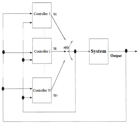
with Ar(t)= A +N1(1 r(t))BD 1C and random signal r(t) 2 M = f1; 2; :::; Ng. This system is represented schematically as
Figure 1. Dynamical system with Markovian switched controller.
We start a stochastic counterpart of the results obtained in [11] and [12] by considering a N states Markovian switched controller of the system in order to be able to perform some useful simulations, and prove stochastic stability under a Markovian transition rule rather than an arbitrary switching. Which means that we deal with the weaker notion of stability than the guaranteed one considered in [11].
3. Formulation
Throughout this paper, we denote n dimensional identity matrix by In or just I. R and C denote the …eld of real and complex numbers respectively. The space
of n n matrices with real entries is denoted by Rn n. We denote a state space representation of the m m transfer function matrix G(s) = C(sI A) 1B + D by (A; B; C; D), where we always assume that A 2 Rn n, B 2 Rn m has full column rank, C 2 Rm n has full row rank, and 0 < D = DT 2 Rm m for some integers
n m.
We also use jyj to denote the Euclidean norm for a row or column vector y, vT is the transpose of v 2 Rn1 n2 with n
i 1. For Z 2 Rn n being a square symmetric matrix, we use max(Z) and min(Z) to denote the maximum and minimum eigen-value of Z respectively.
Let us consider a dynamical linear system with random switching in a probability space ( ; F; P r), and assume that its state equation is described by the following di¤erential equation
_x(t) = Ar(t)x(t); x(0); r(0) = (x0; r0) 2 Rn M; (4) where x(t) is the continuous state, Ar(t)= A+N1(1 r(t))BD
1
C, and fr(t); t 0g is a Markovian jump process with values in a …nite state space M = f1; 2; :::; Ng. r(t) describes the switching between the N modes. Its evolution is governed by the following probability transition
P r(r(t + t) = j=r(t) = i) = (
qij t + o( t) if i 6= j; 1 + qii t + o( t) otherwise,
(5) where qij is the transition rate from mode i to j such that i; j 2 M with qij 0 when i 6= j, and qii=
2 P j=1;j6=i
qij and o( t) is such that lim t!0
o( t) t = 0.
The jump process r(t) has a constant generator Q = (qij) and the process (x(t); r(t)) de…ned by (4) and (5), is associated with an in…nitesimal operator L de…ned as follows:
For each i 2 M and any g(:; i) 2 C1(Rn)
Lg(x; i) = hAix; rg(x; i)i + Qg(x; :)(i);
where h:; :i is the usual inner product in Rn, rg(x; i) denote the gradient (with respect to the variable x) of g(x; i) and Qg(x; :)(i) = P
j2M
qijg(x; j).
Assume that the Markov chain r(t) is irreducible in the sense that the system of equations
( Q = 0
1= 1 (6)
has a unique positive solution, where 1 is a column vector with all component being 1. The positive solution is termed a stationary distribution.
It is known that if P is a transition matrix of a irreducible Markov chain, then, lim n!1P n= 0 B B B B @ 1 2 : : : N : : : : : : : : : 1 2 : : : N 1 C C C C A; where = ( 1; 2; :::; N) is a stationary distribution satisfying
P = :
In the sequel, we will be interested by determining a Lyapunov function for the class of random switching Systems (4), with Ar(t) is a Hurwitz matrix valued function taking values Ai; i 2 f1; 2; :::; Ng which are related through a transfer function matrix.
We recall that it is known that the theoretical justi…cation of stability for this kind of random switching systems can be assured only through the existence of a suitable Lyapunov function.
De…nition 3.1. [12] An m m rational transfer function matrix G(s) is said to be strictly positive real (SPR) if there exists a real scalar > 0 such that G(s) is analytic for Re(s) , and
G(j! ) + GT( j! ) 0; 8! 2 R:
Now, we give a lemma which relates the property of G(s) is SPR and the state space realization (A; B; C; D) when G is a symmetric transfer matrix.
Lemma 3.1. [12] Given a Hurwitz matrix A, the symmetric transfer function matrix G(s) = C(sI A) 1B + D with D = DT > 0 is SPR if and only if A(A BD 1C) has no real negative eigenvalue.
Furthermore, if (A; B; C; D) is a minimal realization of G(s), then the su¢ cient condition is also necessary.
Lemma 3.2. [8] The pair (A; B) is controllable if and only if rank B; AB; :::; An 1B = n: The pair (A; C) is observable if and only if
rank CT; ATCT; :::; (AT)n 1CT = n:
Let us now recall respectively the de…nitions of stochastically ( mean square ) stability and ( asymptotic ) almost surely stability.
(1) stochastically (mean square) stable if for any initial state x0 and initial distribution , we have
Z +1 0
E fjx(t; x0; r0)j2gdt < +1:
(2) (asymptotically) almost surely stable if for any initial state x0 and initial distribution , we have
P rf limt
!+1jx(t; x0; r0)j = 0g = 1:
Lemma 3.3 ([22] page 81). Any mean square stable jump linear system is almost surely stable.
Before displaying the main result, let us given a basic result in systems theory by Kalman-Yakubovic-Popov (KYP). It gives algebraic conditions for the existence of a certain type of Lyapunov function for …rst state.
Lemma 3.4 (KYP). [12] Let A be Hurwitz, (A; B) be controllable, and (A; C) be observable. Then, G(s) = C(sI A) 1B + D is SPR if and only if there exist matrices P = PT > 0, L, W , and a number > 0 satisfying
ATP + P A + P = LTL BTP + WTL = C
D + DT = WTW .
4. Main result
In this section, we present our main result in this paper concerning stochastic stability (Asymptotic almost surely stability) for System (4) by using Lyapunov function. We give su¢ cient conditions which guarantee stochastic stability under some conditions on the transfer matrix G(s).
Theorem 4.1. Assume that the transfer function matrix G(s) is SPR, with (A; B) controllable and (A; C) observable. Then the dynamical random switching System (4) is asymptotically almost surely stable.
Proof. Let us consider the arbitrary square matrices of order n, Piand Pjsatisfying Pi = Pj = P = PT > 0 for i 6= j on M. We de…ne a Lyapunov function by the following expression
At time t, let x(t) = x and r(t) = i 2 M: The in…nitesimal operator acting on V (:; :) and emanating from the point (x; i) at time t is given by
LV (x; i) = hAix; rV (x; i)i + QV (x; :)(i) = xTATi @ @xV (x; i) + X j2M qijV (x; j) = xT ATiPi+ PiAi x + xT X j2M qijPjx = xT (A + 1 N(1 i)BD 1C)TP i+ Pi(A + 1 N(1 i)BD 1C) x; with P j2M
qijPj = 0, because Pi = Pj; 8i; j 2 M and P j2M
qij = 0. Now, we show that for any i 2 M, LV (x; i) 0:The matrix G(s) is SPR, (A; B) and (A; C) are controllable and observable respectively, then, by Lemma 3.4, there exist P = PT > 0, L, W and > 0 such that
ATP + P A = P LTL (7) BTP + WTL = C (8) D + DT = WTW: (9) We …rst take i = 1. By (7), we have LV (x; 1) = xT(A + 1 N(1 1)BD 1C)TP 1+ P1(A + 1 N(1 1)BD 1C)x = xT(ATP + P A)x = xT( P + LTL)x < 0: For i = 2, we get LV (x; 2) = xT (A + 1 N(1 2)BD 1C)TP 2+ P2(A + 1 N(1 2)BD 1C) x = xT (AT 1 N(BD 1C)T)P + P (A 1 N(BD 1C)) x = xT ATP 1 NC TD 1BTP + P A 1 NP BD 1C x: By (7), (8) and (9), we infer LV (x; 2) = xT P LTL 1 NC TD 1(C WTL) 1 N(C W TL)TD 1C x = xT P LTL 1 NC TD 1C + 1 NC TD 1WTL 1 NC TD 1C + 1 NL TW D 1C x
xT P 1 NL TL 1 NC TD 1C + 1 NC TD 1WTL 1 NC TD 1C + 1 NL TW D 1C x xT P 1 NL T(L W D 1C) + 1 NC TD 1WTL 1 NC TD 1WTW D 1C x xT P 1 NL T(L W D 1C) + 1 NC TD 1WT(L W D 1C) x xT P 1 N(L W D 1C)T(L W D 1C) x xT P + 1 N(L W D 1C)T(L W D 1C) x 0: For i = 3, we have LV (x; 3) = xT (A + 1 N(1 3)BD 1C)TP 3+ P3(A + 1 N(1 3)BD 1C) x = xT (AT 2 NBD 1C)TP + P (A 2 NBD 1C) x = xT ATP 2 NC TD 1BTP + P A 2 NP BD 1C x: By (7), (8) and (9), we infer LV (x; 3) = xT P LTL 2 NC TD 1(C WTL) 2 N(C W TL)TD 1C x = xT P LTL 2 NC TD 1C + 2 NC TD 1WTL 2 NC TD 1C + 2 NL TW D 1C x xT P 2 NL TL 2 NC TD 1C + 2 NC TD 1WTL 2 NC TD 1C + 2 NL TW D 1C x xT P 2 NL T(L W D 1C) + 2 NC TD 1WTL 2 NC TD 1WTW D 1C x
xT P 2 NL T(L W D 1C) + 2 NC TD 1WT(L W D 1C) x xT P 2 N(L W D 1C)T(L W D 1C) x xT P + 2 N(L W D 1C)T(L W D 1C) x 0:
By the same argument as steps above, we can show that for any i 2 M = f2; :::; Ng LV (x; i) xT P +i 1 N (L W D 1C)T(L W D 1C) x 0: Let Mi= ( P + LTL for i = 1 P +i 1 N (L W D 1C)T(L W D 1C) for i 2; then, for any i 2 M = f1; 2; :::; Ng, we have
LV (x; i) xTMix; where Mi is positive de…ned. That is
LV (x; i) min
i2M min Mi x Tx: By Dynkin’s formula, we get
E V (x; i) V (x0; r0) = E Z t 0 LV x(s); r(s) ds min i2M min Mi E Z t 0 xT(s)x(s)ds=(x0; r0) ; then min i2M min Mi E Z t 0 xT(s)x(s)ds=(x0; r0) V (x0; r0) E V (x(t); i) V x0; r0 :
This yields that E Z t 0 xT(s)x(s)ds=(x0; r0) V x0; r0 mini2M min Mi : Letting t ! 1, then E Z +1 0 jx(s)j 2ds=(x 0; r0) C(x0; r0); where C(x0; r0) = V (x0;r0) min i2M min Mi
. This means that the trivial solution of System (4) is stochastically (mean square) stable. By Lemma 3.3, System (4) is (asymp-totically) almost surely stable. The proof of the theorem is complete.
Remark 4.1. We remark that if System (4) is 1-dimensional, then, G(s) is a transfer function value, and the pairs (A; B) and (A; C) are always controllable and observable respectively. So, we have the following corollary basing on Lemma 3.1 Corollary 4.2. Let the continuous state x(t) of System (4) be 1-dimensional and A be a Hurwitz matrix, then, the equilibrium point x = 0 is asymptotically almost surely stable if
A(A BD 1C) 0:
Now, we display two examples to demonstrate the applicability and e¤ectiveness of our theoretical result.
5. Examples
In this section, we give two examples to illustrate our result.
Example 5.1. In this example, we consider G(s) symmetric in order to verify easily that it is SPR.
Consider System (4) associated to the symmetric transfer matrix G(s) = C(sI A) 1B + D, with A = 0 @ 2 1 1 0 1 A ; B = 0 @2 1 1 1 1 A ; C = 0 @ 1 2 0:3 0:3 1 A and D = 0 @1 0 0 2 1 A : The Markov jump process r(t) takes values in M = f1; 2; :::; 5g with generator
Q = 0 B B B B @ 4 0 1 1 2 1 2 0 1 0 6 1 8 0 1 0 1 1 3 1 2 1 1 1 5 1 C C C C A: The stationary distribution of irreducible Markov process r(t) is
= (0:27; 0:24; 0:09; 0:23; 0:17), which is obtained by solving Equation (6). Note that the …ve Hurwitz matrices associated to System (4) are given by
Ai= A + (1 i) 5 BD 1C; for i 2 f1; 2; :::; 5g: Then, we have A1= 0 @ 2:0000 1:0000 1:0000 0:0000 1 A ; A2= 0 @ 2:2350 1:6310 0:8330 0:3650 1 A ; A3= 0 @ 2:4700 2:2620 0:6660 0:7300 1 A ; A4= 0 @ 2:7050 2:8930 0:4990 1:0950 1 A
and A5= 0 @ 2:9400 3:5240 0:3320 1:4600 1 A :
The hybrid System (4) becomes a switching system associated with …ve ordinary di¤ erential equations
_x(t) = 8 > > > > > > < > > > > > > : A1x(t) : : : A5x(t); (10)
switching back and forth from one to another according to the movement of the jump process r(t). Note that (A; B) and (A; C) are controllable and observable re-spectively; rank([B; AB]) = 2 and rank([CT; ATCT]) = 2 . The transfer function G(s) = C(sI A) 1B + D is symmetric G(s) = 1 (s2+ 2:9s + 2:425) 0 @s 2+ 6:9s + 9:535 s 1 s 1 2s2+ 5:8s + 4:7 1 A
and A(A BD 1C) has no real negative eigenvalue, that means that G(s) is SPR. Then, by Theorem 4.1 the hybrid System (10) is asymptotically almost surely stable.
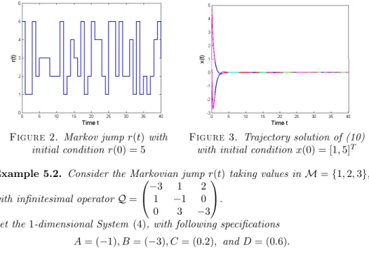
Figure 2. Markov jump r(t) with initial condition r(0) = 5
Figure 3. Trajectory solution of (10) with initial condition x(0) = [1; 5]T Example 5.2. Consider the Markovian jump r(t) taking values in M = f1; 2; 3g, with in…nitesimal operator Q =
0
@ 13 11 20
0 3 3
1 A.
Let the 1-dimensional System (4), with following speci…cations A = ( 1); B = ( 3); C = (0:2); and D = (0:6):
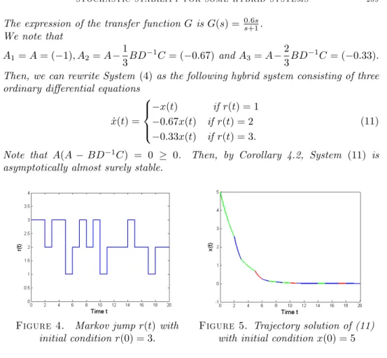
The expression of the transfer function G is G(s) = 0:6s s+1. We note that A1= A = ( 1); A2= A 1 3BD 1C = ( 0:67) and A 3= A 2 3BD 1C = ( 0:33): Then, we can rewrite System (4) as the following hybrid system consisting of three ordinary di¤ erential equations
_x(t) = 8 > < > : x(t) if r(t) = 1 0:67x(t) if r(t) = 2 0:33x(t) if r(t) = 3: (11)
Note that A(A BD 1C) = 0 0. Then, by Corollary 4.2, System (11) is asymptotically almost surely stable.
Figure 4. Markov jump r(t) with initial condition r(0) = 3:
Figure 5. Trajectory solution of (11) with initial condition x(0) = 5 Acknowledgments
The author would like to thank B. Benaid, H. Bouzahir, F. El Guezar and M. Aatabe for extensive helpful discussions.
References
[1] M. Balde, U. Boscain and P. Mason, A note on stability conditions for planar switched systems, Internat. J. Control 82, no. 10, (2009) pp. 1882-1888.
[2] M. Benaîm, S. Le Borgne, F. Malrieu and P. A. Zitt, On the stability of planar randomly switched systems, Annals of Applied Probability, Institute of Mathematical Statistics (IMS), 24 (1), (2014) pp. 292-311.
[3] H. Bouzahir and X. Fu, Controllability of neutral functional di¤erential equations with in…nite delay, Acta Mechanica Sinica, 31(1), (2011) pp. 73-80.
[4] O. L. V. Costa, M. D. Fragoso and M. G. Todorov, continuous-time Markov jump linear systems, Springer-Verlag Berlin Heidelberg 2013.
[5] F. El Guezar, H. Bouzahir and D. Fournier-Prunaret, Event detection occurrence for planar piece-wise a¢ ne hybrid systems, Nonlinear Anal. Hybrid Syst. 5 no. 4 (2011), pp. 626-638.
[6] F. El Guezar and H. Bouzahir, Simulation of piecewise hybrid dynamical systems in Matlab, In "MATLAB, A Fundamental Tool for Scienti…c Computing and Engineering Applications, Volume ", InTech, 2012.
[7] C. Imzegouan, H. Bouzahir, B. Benaid and F. El Guezar, A note on exponential sto-chastic stability of Markovian switching Systems, International Journal of Evolution Equations, Vol 10, Issue 2, (2016), pp. 189-198.
[8] Z. H. Guan, T. H. Qian and X. Yu, On controllability and observability for a class of impulsive systems, Systems Control Lett. 47 (2002) pp. 247-257.
[9] R. A. Horn, and C. R. Johnson, Matrix analysis, Cambridge university Press, 1990.
[10] T. Kailath, Linear systems, Englewood Cli¤s, NJ: Prentice Hall. (1980).
[11] Y. Kouhi, N. Bajcinca, J. Raisch and R. Shorten, A new stability result for switched linear systems, Proceedings of the European control conference, (2013) pp. 2152-2156.
[12] Y. Kouhi, N. Bajcinca, J. Raisch and R. Shorten, On the quadratic stability of switched linear systems associated with symmetric transfer function matrices, Au-tomatica J. IFAC 50, no. 11, (2014) pp. 2872-2879.
[13] L. Knockaert, F. Ferranti and T. Dhaene, Generalized eigenvalue passivity assessment of descriptor systems with applications to symmetric and singular systems, Interna-tional Journal of Numerical Modeling: Electronic Networks, Devices and Fields, 26 (1), (2013) pp. 1-14.
[14] X. Mao, Stability of stochastic di¤erential equations with Markovian switching, Sto-chastic Process. Appl. 79, no. 1 (1999) pp. 45-67.
[15] L. Perko, Di¤erential equations and dynamical systems, Springer, 3rd Ed., New York, (2001).
[16] A. Rantzer, On the Kalman-Yakubovich-Popov lemma, Systems and Control Letters 28 (1996) pp. 7-10.
[17] Z. Sun and S. S. Ge, Stability theory of switched dynamical systems, Springer-Verlag London Limited, 2011.
[18] R. N. Shorten and K. S. Narendra, On common quadratic Lyapunov functions for pairs of stable LTI systems whose system matrices are in companion form, IEEE Transactions on Automatic Control, 48(4) (2003) pp. 618-621.
[19] G. Yin and C. Zhu, On the notion of weak stability and related issues of hybrid di¤usion systems, Nonlinear Anal.: Hybrid Sys. 1, no. 2 (2007) pp. 173-187.
[20] G. Yin, G. Zhao and F. Wu, Regularization and stabilization of randomly switching dynamic systems, SIAM J. Appl. Math. Vol. 72, no. 5 (2012) pp. 1361-1382
[21] C. Yuan and X. Mao, Asymptotic stability in distribution of stochastic di¤erential equations with Markovian switching, Stochastic Process. Appl. 103, no. 2 (2003) pp. 277-291.
[22] S. Zhendong and S. G. Shuzhi, Stability theory of switched dynamical systems, Com-munications and Control Engineering Series. Springer, London, 2011.
[23] C. Zhu, G. Yin and Q. S. Song, Stability of random-switching systems of di¤erential equations, Quart. Appl. Math. 67, no. 2 (2009) pp. 201-220.
Current address : ISTI Lab, ENSA PO Box 1136 Agadir, MOROCCO E-mail address : [email protected]