Optical fractional spherical magnetic flux flows with Heisenberg spherical Landau Lifshitz model

(1)

Available online 24 March 2021

Original research article

Optical fractional spherical magnetic flux flows with Heisenberg

spherical Landau Lifshitz model

Talat K¨orpinar

a,

_{*, Zeliha K¨orpinar}

b

a_{Mus¸ Alparslan University, Department of Mathematics, 49250, Mus¸, Turkey} b_{Mus¸ Alparslan University, Department of Administration, 49250, Mus¸, Turkey}

A R T I C L E I N F O Keywords:

Sα-magnetic particle

Heisenberg spherical Landau Lifshitz model Geometric magnetic flux density PACS:

04.20.− q 03.50.De 02.40.− k

A B S T R A C T

In this paper, we first offer the approach of spherical magnetic Lorentz flux of spherical Sα-magnetic particle flows by the spherical frame in spherical Heisenberg space S2ℍ. Eventually, we obtain some optical conditions of spherical Sα-magnetic Lorentz flux by using directional spherical fields. Moreover, we determine spherical magnetic Lorentz flux for spherical vector fields. Also, we give new construction for spherical curvatures of spherical Sα-magnetic particle flows by considering Heisenberg spherical Landau Lifshitz model. Finally, magnetic flux surface is demonstrated in a static and uniform magnetic surface by using the analytical and numerical results with Heisenberg spherical Landau Lifshitz model.

1. Introduction

Differential geometric tools such as surfaces and curves have been appeared in many disciplines of theoretical and practical areas of science ranging from thermodynamics [1] to high energy strings [2], and from general relativity [3] to solitons [4], or even in plasma physics [5] and liquid crystals [6]. The motion of curves and the concept of the Frenet–Serret frame are the main common ingredient in all these applications.

These tools have also been considered in the research of magnetic structures significantly. Recently, many authors have focused on the subject of magnetic curves and investigate many important results. In these studies, one common approach has been used extensively. According to this approach, it is generally assumed that magnetic curves are trajectories of the time-independent moving charged particle on geometric manifolds or physical spacetime structures. This motion of the particle is specifically determined by the Lorentz force equation. Once the Lorentz force equation is managed to solve successfully, then many interesting characterizations have been developed from the geometric and physical points of view [7–15].

These structures implemented by many authors to define magnetic flux-tubes in the case of inflexional configuration and inflec-tional disequilibrium. In the presence of a magnetic field, the magnetic flux-tube is defined by the cylindrical thin tube of circular cross- section having a positive radius. The cases of twisted magnetic flux-tube and straight flux-tube are investigated separately in various studies. The geometric formulation of these tubes is derived by the Lorentz force equation and used to determine generic charac-terizations associated with the several useful applications to astrophysical flows, solar corona loops, etc. Nested toroidal flux surface is described due to the motion curves in magnetohydrostatic. It can be considered as a generalization of the magnetic flux-tube. All these results have been obtained through the Riemannian and non-Riemannian geometric data and facts [16–20].

* Corresponding author.

E-mail address: talatkorpinar@gmail.com (T. K¨orpinar).

Contents lists available at ScienceDirect

Optik

journal homepage: www.elsevier.com/locate/ijleo

https://doi.org/10.1016/j.ijleo.2021.166634

(2)

In recent times there have been diverse developments in the operation of geometric flux flows from computer perspective, which has both analytical and functional significance. Some researchers have desired to derive flux flows that take into account the optical surfaces of fields enclosed by flows magnetic particles [21–26].

The geometric phase investigation along the optical fiber investigation is mostly conducted by observing the action of electro-magnetic particles and their features. Some nonlinear evolution structures are frequently encountered particularly in genuine-state physics, chemical physics, plasma physics, optical physics, fluid mechanics, etc. Even though these equations have been heavily used in many structures, it requires very hard work to obtain the explicit solutions of approximate systems. Thus, there exists no global or unified approach to demonstrate the exact solutions of all nonlinear transformation systems [27–37].

The aim of the present paper is to study the effect of the geometric interpretation of the notion of the Heisenberg spherical ferromagnetic spin for spherical flows of magnetic particles with the spherical-frame in spherical Heisenberg space S2_{ℍ. Eventually, we} obtain some optical conditions of spherical Sα− magnetic Lorentz flux by using spherical fields. Moreover, we determine spherical magnetic Lorentz flux for spherical fields. Also, we give new conditions for spherical potentials of spherical Sα− magnetic flows by considering Heisenberg spherical Landau Lifshitz model. Finally, the magnetic flux surface is demonstrated in a static and uniform magnetic surface by using the analytical and numerical results with Heisenberg spherical Landau Lifshitz model.

2. Backround on the spherical frame in S2 ℍ Heisenberg metric g is given via

g = dx2₊_dy2_{+ (dz − xdy)}2_.

Basis for Lie algebra of Heisenberg group is given by e1= ∂ ∂x, e2= ∂ ∂y+x ∂ ∂z, e = ∂ ∂z.

Let α: I→ S2ℍ be unit speed smooth particle. Spherical frame system is defined by spherical frame ⎡ ⎣∇_∇σ_σα_t ∇σs ⎤ ⎦ = ⎡ ⎣₋0₁ 1₀ 0_ε 0 − ε 0 ⎤ ⎦ ⎡ ⎣α_t s ⎤ ⎦, where ε=det(α,t,∇σt).

Also, the particle satisfying this spherical frame equations is defined Lorentzian spherical particle. The vector products of spherical fields are given by

α=t × s, t = s ×α, s =α×t.

3. Flows of Sα-magnetic particles in spherical Heisenberg space S2ℍ

In this section, it is first described magnetic surfaces with the time evolution of the spherical Sα-magnetic particle in spherical Heisenberg space S2_{ℍ. The time evolution is assumed to be a new design embedded in the spherical space. Thus, the fundamental} geometric construction of the flows as surfaces can naturally be induced by moving spherical orthonormal fields.

♠ Let α be smooth particle with magnetic field ℬ in the spherical Heisenberg space S2ℍ.We call particle α as a spherical Sα-magnetic particle if the spherical tangent field with the following equation:

∇σα=ϕ(α) = ℬ ×α.

♠ Lorentz force ϕ for spherical Sα-magnetic particle is given ϕ(α) = π2ϖe1− π1ϖe2+cosφe3,

ϕ(t) = − (π1+sin3φ)e1+ (− π2+ωπ4)e2− (π3+sin3φ)e3, ϕ(s) = − ωπ2ϖe1+ωπ1ϖe2− ωcosφe3,

where ω=g(ϕ(t), s) is a sufficiently smooth function. Also, magnetic field ℬ is given by ℬ = (π1ω− 1 ϖsin 3_φ)e 1+ (π2ω+χ4)e2+ (π3ω− 1 ϖsin 3_φ)e 3, where

(3)

π1 = − 1 ϖsinφcos[ϖσ+ϖ1], π2 = 1 ϖsinφsin[ϖσ+ϖ1], π3 = (cosφ − 1 ϖsin 2_φ)_σ₋ 1 4ϖ2sin 2_φsin2[ϖ_σ₊_ϖ 1], π4 = ( 1 ϖsin 2_φcos[ϖ_σ₊_ϖ 1]cosφ + sinφsin[ϖσ+ϖ1]χ3), ϖ = ( ̅̅̅̅̅̅̅̅̅̅̅̅̅ 1 +ε2 √ sinφ − cosφ).

Let α(σ,t) be the motion of regular spherical Sα-magnetic particle in spherical Heisenberg space S2ℍ. The flow of spherical Sα-magnetic particle is given by

∇tα=χ1t +χ2s,

where χ₁,χ₂are potentials of particle. ♠Time derivatives of spherical frame

∇tα = (χ1π2ϖ − χ2 ϖsin 3_φ)e 1− (χ1π1ϖ − χ2π4)e2 +(χ1cosφ − χ2 ϖsin 3_φ)e 3, ∇tt = − (χ1π1+ 1 ϖ(χ1ε+ ∂χ2 ∂σ)sin 3_φ)e 1+ (π4(χ1ε +∂χ2 ∂σ) − χ1π2)e2− (χ1π3+ 1 ϖ(χ1ε+ ∂χ2 ∂σ)sin 3_φ)e 3, ∇ts = − (χ2π1+π2ϖ(χ1ε+ ∂χ2 ∂σ))e1+ (π1ϖ(χ1ε+ ∂χ2 ∂σ) − χ2π2)e2− (χ2π3+cosφ(χ1ε+ ∂χ2 ∂σ))e3.

♠Flows of ϕ(α),ϕ(t), ϕ(s) forces of the spherical frame are presented by ∇tϕ(α) = − (χ1π1+ 1 ϖ(χ1ε+ ∂χ2 ∂σ)sin 3_φ)e 1− (χ1π2− π4(χ1ε +∂χ2 ∂σ))e2− (χ1π3+ 1 ϖ(χ1ε+ ∂χ2 ∂σ)sin 3_φ)e 3, ∇tϕ(t) = − ((ω(χ1ε+ ∂χ2 ∂σ) +χ1)π2ϖ +ωχ2π1+ 1 ϖ( ∂ω ∂t− χ2)sin3φ)e1 +((ω(χ1ε+ ∂χ2 ∂σ) +χ1)π1ϖ − ωχ2π2+π4(∂ω ∂t − χ2))e2 − ((ω(χ1ε+ ∂χ2 ∂σ) +χ1)cosφ +ωχ2π3+ 1 ϖ( ∂ω ∂t − χ2)sin3φ)e3, ∇tϕ(s) = ( ω ϖ(χ1ε+ ∂χ2 ∂σ)sin 3_{φ −} _π 2ϖ ∂ω ∂t +ωχ1π1)e1+ (π1ϖ ∂ω ∂t +ωχ1π2 − π4ω(χ1ε+ ∂χ2 ∂σ))e2+ ( ω ϖ(χ1ε+ ∂χ2 ∂σ)sin 3_{φ +}_ωχ 1π3− cosφ∂ω ∂t)e3. 4. Spherical magnetic Lorentz flux surfaces

The magnetic flux equation theory or the theory of flux systems has had an enormous impact on applied physical and mathematical studies. This framework combines some subtle techniques in nonlinear flux optics, field designs and sigma models, fluid dynamics, relativity, electromagnetic wave theory. In this section, we obtain spherical magnetic ϕ(α),ϕ(t), ϕ(s) flux conditions by using the Heisenberg spherical Landau Lifshitz model.

Case 1. Spherical magnetic ϕ(α)flux with Heisenberg spherical Landau Lifshitz model Theorem 4.1. The spherical Heisenberg magnetic ϕ(α)fluxmℱℒℒϕ(α)is given by

(4)

m_ℱℒℒ ϕ(α) = ∫ ℱ (− π1ϖε(π2ω+χ4) ∂ε ∂σ+π2ϖε(π1ω − 1 ϖsin 3_φ)∂ε ∂σ+cosφε(π3ω− 1 ϖsin 3_φ)∂ε ∂σ)dv. Proof. From definition of spherical Heisenberg magnetic ϕ(α)flux

m_ℱ ϕ(α)=

∫ ℱ

ℬ⋅ ∇sϕ(α) × ∇tϕ(α)dv.

By short calculations, we have ∇σϕ(α) × ∇tϕ(α) =π2ϖ ∂χ2 ∂σe1− π1ϖ ∂χ2 ∂σe2+cosφ ∂χ2 ∂σe3. Magnetic flux density of ϕ(tq)is given by

m_ℒ ϕ(α)=π2ϖ(π1ω− 1 ϖsin 3_φ)∂χ2 ∂σ− π1ϖ(π2ω+χ4) ∂χ2 ∂σ+cosφ(π3ω− 1 ϖsin 3_φ).

Moreover, ϕ(α)flux is obtained in the following way

m_ℱ ϕ(α)= ∫ ℱ (− π1ϖ(π2ω+χ4) ∂χ2 ∂σ+π2ϖ(π1ω− 1 ϖsin 3_φ)∂χ2 ∂σ+cosφ(π3ω− 1 ϖsin 3_φ))dv.

From Landau Lifshitz model, flux density is given by

m_ℒℒℒ ϕ(α)= ℬ⋅ ∇sϕ(α) ×ϕ(α) × ∇2sϕ(α). Also, we get ϕ(α) × ∇2σϕ(α) =π1 ∂ε ∂σe1+π2 ∂ε ∂σe2+π3 ∂ε ∂σe3. Similarly, we can obtain that

∇σϕ(α) ×ϕ(α) × ∇2σϕ(α) =π2ϖε ∂ε ∂σe1− π1ϖε ∂ε ∂σe2+cosφε ∂ε ∂σe3. Spherical Landau Lifshitz magnetic ϕ(α)flux is given by

m_ℒℒℒ ϕ(α)=π2ϖε(π1ω− 1 ϖsin 3_φ)∂ε ∂σ− π1ϖε(π2ω+χ4) ∂ε ∂σ+cosφε(π3ω− 1 ϖsin 3_φ)∂ε ∂σ. From above equation, we have

m_ℱℒℒ ϕ(α)= ∫ ℱ (− π1ϖε(π2ω+χ4) ∂ε ∂σ+π2ϖε(π1ω− 1 ϖsin 3_φ)∂ε ∂σ+cosφε(π3ω− 1 ϖsin 3_φ)∂ε ∂σ)dv. This proves the theorem.

In the light of Theorem 3.1, we express the following important results. •The Heisenberg magnetic ϕ(α)flux surface condition is given by

π2ϖ(π1ω− 1 ϖsin 3_φ)∂χ2 ∂σ− π1ϖ(π2ω+χ4) ∂χ2 ∂σ+cosφ(π3ω− 1 ϖsin 3_{φ) = 0.}

•The Heisenberg magnetic ϕ(α)Landau Lifshitz flux surface is presented by π2ϖε(π1ω− 1 ϖsin 3_φ)∂ε ∂σ− π1ϖε(π2ω+χ4) ∂ε ∂σ+cosφε(π3ω− 1 ϖsin 3_φ)∂ε ∂σ=0. Therefore, we have the following corollary.

Corollary 1. Gauss’s law of the ϕ(α)Landau Lifshitz flux closed surface is presented by ∮ S (− π1ϖε(π2ω+χ4) ∂ε ∂σ+π2ϖε(π1ω− 1 ϖsin 3_φ)∂ε ∂σ+cosφε(π3ω− 1 ϖsin 3_φ)∂ε ∂σ)dv = 0.

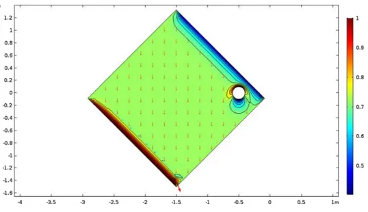
For numerical work, the above systems are often used spherical magnetic flux density. Spherical magnetic ϕ(α)Landau Lifshitz flux is usually derived using the properties of the divergence-free nature of the magnetic field along with the definition of the spherical magnetic flux density in spherical Heisenberg space S2_{ℍ. To obtain the visualization of the evolved systems of the magnetic ϕ(}_α₎_flux

m_ℱ

(5)

results of the magnetic ϕ(α)flux mℱϕ(α)on the spherical magnetic flux density and magnetic field of an ideal conductor at minimum density are illustrated in Fig. 1.

Case 2. Spherical Magnetic ϕ(t) flux with Heisenberg spherical Landau Lifshitz model Theorem 4.2. The spherical Heisenberg magnetic ϕ(t) Landau Lifshitz flux m_ℱℒℒ

ϕ(t)is given by m_ℱℒℒ ϕ(t)= ∫ ℱ ((π2ω+χ4)(π4ω(ωε+1)(ω∂ε ∂σ+2 ∂ω ∂σε) − π1ϖω ∂ω ∂σ(ω ∂ ∂σε +2∂ω ∂σε) − η2π2) + (π1ω− 1 ϖsin 3_φ)(_π 2ϖω ∂ω ∂σ(ω ∂ ∂σε+2 ∂ω ∂σε) − η2π1 − 1 ϖω(ωε+1)(ω ∂ε ∂σ+2 ∂ω ∂σε)sin 3_{φ) + (}_π 3ω− 1 ϖsin 3_φ)(cosφ_ω∂ω ∂σ(ω ∂ ∂σε +2∂ω ∂σε) − 1 ϖω(ωε+1)(ω ∂ε ∂σ+2 ∂ω ∂σε)sin 3_{φ −} _η 2π3))dv.

Proof. From Lorentz force equation, we have ∇σϕ(t) × ∇tϕ(t) = ( 1 ϖ(ωε+1)ωχ2sin3φ +η1π1− π2ϖωχ2 ∂ω ∂σ)e1 +(π1ϖωχ2 ∂ω ∂σ− π4(ωε+1)ωχ2+η1π2)e2 +(1 ϖ(ωε+1)ωχ2sin3φ +η1π3− cosφωχ2 ∂ω ∂σ)e3, where η1= ∂ω ∂σ(ω(χ1ε+ ∂χ2 ∂σ) +χ1) − (ωε+1)( ∂ω ∂t− χ2). m_ℒ ϕ(t) = ( 1 ϖ(ωε+1)ωχ2sin3φ +η1π1− π2ϖωχ2 ∂ω ∂σ)(π1ω− 1 ϖsin 3_φ) +(π2ω+χ4)(π1ϖωχ2 ∂ω ∂σ− π4(ωε+1)ωχ2+η1π2) +(1 ϖ(ωε+1)ωχ2sin3φ +η1π3− cosφωχ2 ∂ω ∂σ)(π3ω− 1 ϖsin 3_φ). Then, m_ℱ ϕ(t)is given by

(6)

m_ℱ ϕ(t) = ∫ ℱ ((π1ϖωχ2 ∂ω ∂σ− π4(ωε+1)ωχ2+η1π2)(π2ω+χ4) +(π1ω− 1 ϖsin 3_φ)(1 ϖ(ωε+1)ωχ2sin3φ +η1π1− π2ϖωχ2 ∂ω ∂σ) +(1 ϖ(ωε+1)ωχ2sin3φ +η1π3− cosφωχ2 ∂ω ∂σ)(π3ω− 1 ϖsin 3_φ))dv.

In a similar way, we get

∇σϕ(t) × ϕ(t) × ∇2σϕ(t) = (π2ϖω ∂ω ∂σ(ω ∂ ∂σε+2 ∂ω ∂σε) − η2π1− 1 ϖω(ωε+1)(ω ∂ε ∂σ +2∂ω ∂σε)sin 3_φ)e 1+ (π4ω(ωε+1)(ω∂ε ∂σ+2 ∂ω ∂σε) − π1ϖω ∂ω ∂σ(ω ∂ ∂σε+2 ∂ω ∂σε) − η2π2)e2+ (cosφω ∂ω ∂σ(ω ∂ ∂σε+2 ∂ω ∂σε) − 1 ϖω(ωε+1)(ω ∂ε ∂σ+2 ∂ω ∂σε)sin 3_{φ −} _η 2π3)e3, where η2= ((ω ∂ε ∂σ+2 ∂ω ∂σε)(ωε+1)− ∂ω ∂σ( ∂2_ω ∂σ2+(ωε+1)(ω− ε))). From above equations, we get

m_ℒℒℒ ϕ(t)= (π1ω− 1 ϖsin 3_φ)(_π 2ϖω∂ω ∂σ(ω ∂ ∂σε+2 ∂ω ∂σε) − η2π1− 1 ϖω(ωε +1)(ω∂ε ∂σ+2 ∂ω ∂σε)sin 3_{φ) + (}_π 2ω+χ4)(π4ω(ωε+1)(ω∂ε ∂σ+2 ∂ω ∂σε) − π1ϖω∂ω ∂σ(ω ∂ ∂σε+2 ∂ω ∂σε) − η2π2) + (π3ω− 1 ϖsin 3_φ)(cosφ_ω∂ω ∂σ(ω ∂ ∂σε +2∂ω ∂σε) − 1 ϖω(ωε+1)(ω ∂ε ∂σ+2 ∂ω ∂σε)sin 3_{φ −} _η 2π3). Similarly, magnetic ϕ(t) Landau Lifshitz flux is given by

m_ℱℒℒ ϕ(t)= ∫ ℱ ((π2ω+χ4)(π4ω(ωε+1)(ω ∂ε ∂σ+2 ∂ω ∂σε) − π1ϖω ∂ω ∂σ(ω ∂ ∂σε +2∂ω ∂σε) − η2π2) + (π1ω− 1 ϖsin 3_φ)(_π 2ϖω ∂ω ∂σ(ω ∂ ∂σε+2 ∂ω ∂σε) − η2π1 − 1 ϖω(ωε+1)(ω ∂ε ∂σ+2 ∂ω ∂σε)sin 3_{φ) + (}_π 3ω− 1 ϖsin 3_φ)(cosφ_ω∂ω ∂σ(ω ∂ ∂σε +2∂ω ∂σε) − 1 ϖω(ωε+1)(ω ∂ε ∂σ+2 ∂ω ∂σε)sin 3_{φ −} _η 2π3))dv, which completes the proof of the theorem.

In the light of Theorem 3.2, we express the following important results. •The Heisenberg magnetic ϕ(t) flux surface condition is given by

(1 ϖ(ωε+1)ωχ2sin3φ +η1π1− π2ϖωχ2 ∂ω ∂σ)(π1ω− 1 ϖsin 3_φ) +(π2ω+χ4)(π1ϖωχ2 ∂ω ∂σ− π4(ωε+1)ωχ2+η1π2) +(1 ϖ(ωε+1)ωχ2sin3φ +η1π3− cosφωχ2 ∂ω ∂σ)(π3ω− 1 ϖsin 3_{φ) = 0.}

(7)

(π1ω− 1 ϖsin 3_φ)(_π 2ϖω∂ω ∂σ(ω ∂ ∂σε+2 ∂ω ∂σε) − η2π1− 1 ϖω(ωε +1)(ω∂ε ∂σ+2 ∂ω ∂σε)sin 3_{φ) + (}_π 2ω+χ4)(π4ω(ωε+1)(ω ∂ε ∂σ+2 ∂ω ∂σε) − π1ϖω∂ω ∂σ(ω ∂ ∂σε+2 ∂ω ∂σε) − η2π2) + (π3ω− 1 ϖsin 3_φ)(cosφ_ω∂ω ∂σ(ω ∂ ∂σε +2∂ω ∂σε) − 1 ϖω(ωε+1)(ω ∂ε ∂σ+2 ∂ω ∂σε)sin 3_{φ −} _η 2π3) =0. Therefore, we have the following corollary.

Corollary 2. Gauss’s law of the ϕ(t) Landau Lifshitz flux closed surface is presented by ∮ S ((π2ω+χ4)(π4ω(ωε+1)(ω∂ε ∂σ+2 ∂ω ∂σε) − π1ϖω ∂ω ∂σ(ω ∂ ∂σε +2∂ω ∂σε) − η2π2) + (π1ω− 1 ϖsin 3_φ)(_π 2ϖω∂ω ∂σ(ω ∂ ∂σε+2 ∂ω ∂σε) − η2π1 − 1 ϖω(ωε+1)(ω ∂ε ∂σ+2 ∂ω ∂σε)sin 3_{φ) + (}_π 3ω− 1 ϖsin 3_φ)(cosφ_ω∂ω ∂σ(ω ∂ ∂σε +2∂ω ∂σε) − 1 ϖω(ωε+1)(ω ∂ε ∂σ+2 ∂ω ∂σε)sin 3_{φ −} _η 2π3))dv.

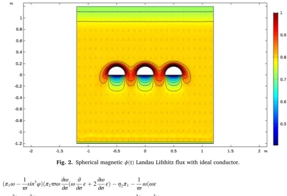
For numerical work, the above systems are often used spherical magnetic flux density. Spherical magnetic ϕ(t) Landau Lifshitz flux is usually derived using the properties of the divergence-free nature of the magnetic field along with the definition of the spherical magnetic flux density. To obtain the visualization of the evolved systems of the magnetic ϕ(t) flux m_ℱ

ϕ(t)we use the basic numerical

algorithms to solve the above equations at Matlab and Comsol software. This approach presents the results of the magnetic ϕ(t) flux

m_ℱ

ϕ(t)on the spherical magnetic flux density and magnetic field of an ideal conductor at minimum density are illustrated in Fig. 2.

Case 3. Spherical magnetic ϕ(s) flux with Heisenberg spherical Landau Lifshitz model Theorem 4.3. The spherical Heisenberg magnetic ϕ(s) Landau Lifshitz flux m_ℱℒℒ

ϕ(s)is given by m_ℱℒℒ ϕ(s)= ∫ ℱ ((π2ω+χ4)(π1ϖ(εω2(ω ∂ε ∂σ+2 ∂ω ∂σε) +2ω 2∂ω ∂σ) − 2ω( ∂ω ∂σ) 2_π 2 +π4ω∂ω ∂σ(ω ∂ε ∂σ+2 ∂ω ∂σε)) − (π1ω− 1 ϖsin 3_φ)(_π 2ϖ(εω2(ω∂ε ∂σ+2 ∂ω ∂σε) +2ω 2∂ω ∂σ) +2ω(∂ω ∂σ) 2 π1+ω ϖ ∂ω ∂σ(ω ∂ε ∂σ+2 ∂ω ∂σε)sin 3_{φ) − (}_π 3ω− 1 ϖsin 3_φ)((_εω2₍_ω∂ε ∂σ +2∂ωε 2ω2∂ω_{cosφ +}ω∂ω_ω∂ε ₂∂ω_ε_sin3_{φ + 2}_ω∂ω2 π3))dv.

(8)

Proof. By some calculations, we have ∇σϕ(s) × ∇tϕ(s) = (π1( ∂ω ∂σω(χ1ε+ ∂χ2 ∂σ) − ωε ∂ω ∂t) +π2ϖ(ω 2₍_χ 1ε+ ∂χ2 ∂σ) − εω 2_χ 1) − 1 ϖ( ∂ω ∂σωχ1− ω ∂ω ∂t)sin 3_φ)e 1+ (π2( ∂ω ∂σω(χ1ε+ ∂χ2 ∂σ) − ωε ∂ω ∂t) − π1ϖ(ω 2₍_χ 1ε +∂χ2 ∂σ) − εω 2_χ 1) +π4( ∂ω ∂σωχ1− ω ∂ω ∂t))(π2ω+χ4) + (π3( ∂ω ∂σω(χ1ε+ ∂χ2 ∂σ) − ωε∂ω ∂t) +cosφ(ω 2₍_χ 1ε+ ∂χ2 ∂σ) − εω 2_χ 1) − 1 ϖ( ∂ω ∂σωχ1− ω ∂ω ∂t)sin 3_φ)e 3. Flux density of ϕ(s) is given by

m_ℒ ϕ(s)= (π1(∂ω ∂σω(χ1ε+ ∂χ2 ∂σ) − ωε ∂ω ∂t) +π2ϖ(ω 2₍_χ 1ε+ ∂χ2 ∂σ) − εω 2_χ 1) − 1 ϖ( ∂ω ∂σωχ1 − ω∂ω ∂t)sin 3_φ)(_π 1ω− 1 ϖsin 3_{φ) + (}_π 2( ∂ω ∂σω(χ1ε+ ∂χ2 ∂σ) − ωε ∂ω ∂t) − π1ϖ(ω 2₍_χ 1ε +∂χ2 ∂σ) − εω 2_χ 1) +π4( ∂ω ∂σωχ1− ω ∂ω ∂t))e2+ (π3( ∂ω ∂σω(χ1ε+ ∂χ2 ∂σ) − ωε ∂ω ∂t) +cosφ(ω2₍_χ 1ε+ ∂χ2 ∂σ) − εω 2_χ 1) − 1 ϖ( ∂ω ∂σωχ1− ω ∂ω ∂t)sin 3_φ)(_π 3ω− 1 ϖsin 3_φ).

Using above equation in phase, we obtain that

m_ℱ ϕ(s)= ∫ ℱ ((π2( ∂ω ∂σω(χ1ε+ ∂χ2 ∂σ) − ωε ∂ω ∂t) − π1ϖ(ω 2₍_χ 1ε+ ∂χ2 ∂σ) − εω 2_χ 1) +π4( ∂ω ∂σωχ1− ω ∂ω ∂t))(π2ω+χ4) + (π1( ∂ω ∂σω(χ1ε+ ∂χ2 ∂σ) − ωε ∂ω ∂t) +π2ϖ(ω 2₍_χ 1ε+ ∂χ2 ∂σ) − εω2_χ 1) − 1 ϖ( ∂ω ∂σωχ1− ω ∂ω ∂t)sin 3_φ)(_π 1ω− 1 ϖsin 3_{φ) + (}_π₃₍∂ω ∂σω(χ1ε+ ∂χ2 ∂σ) − ωε ∂ω ∂t) +cosφ(ω2₍_χ 1ε+ ∂χ2 ∂σ) − εω 2_χ 1) − 1 ϖ( ∂ω ∂σωχ1− ω ∂ω ∂t)sin 3_φ)(_π 3ω− 1 ϖsin 3_φ))dv.

Also, Landau Lifshitz model for ϕ(s), we get that

m_ℒℒℒ

ϕ(s)= ℬ⋅ ∇sϕ(s) × ϕ(s) × ∇2sϕ(s).

By using the relations of Lorentz force, we get ϕ(s) × ∇2 σϕ(s) = (π1ω(ω∂ε ∂σ+2 ∂ω ∂σε) − 2ω ϖ ∂ω ∂σsin 3_φ)e 1+ (π2ω(ω∂ε ∂σ +2∂ω ∂σε) +2ωπ4 ∂ω ∂σ)e2+ (π3ω(ω ∂ε ∂σ+2 ∂ω ∂σε) − 2ω ϖ ∂ω ∂σsin 3_φ)e 3. On the other hand, cross product are

∇σϕ(s) × ϕ(s) × ∇2σϕ(s) = − (π2ϖ(εω2(ω ∂ε ∂σ+2 ∂ω ∂σε) +2ω 2∂ω ∂σ) +2ω( ∂ω ∂σ) 2_π 1 +ω ϖ ∂ω ∂σ(ω ∂ε ∂σ+2 ∂ω ∂σε)sin 3_φ)e 1+ (π1ϖ(εω2(ω ∂ε ∂σ+2 ∂ω ∂σε) +2ω 2∂ω ∂σ) − 2ω(∂ω ∂σ) 2_π 2+π4ω ∂ω ∂σ(ω ∂ε ∂σ+2 ∂ω ∂σε))e2− ((εω 2₍_ω∂ε ∂σ+2 ∂ω ∂σε) +2ω2∂ω ∂σ)cosφ + ω ϖ ∂ω ∂σ(ω ∂ε ∂σ+2 ∂ω ∂σε)sin 3_{φ + 2}_ω₍∂ω ∂σ) 2_π 3)e3. Also, we find that

(9)

m_ℒℒℒ ϕ(s)= − (π1ω− 1 ϖsin 3_φ)(_π 2ϖ(εω2(ω∂ε ∂σ+2 ∂ω ∂σε) +2ω 2∂ω ∂σ) +2ω( ∂ω ∂σ) 2_π 1 +ω ϖ ∂ω ∂σ(ω ∂ε ∂σ+2 ∂ω ∂σε)sin 3_{φ) + (}_π 2ω+χ4)(π1ϖ(εω2(ω∂ε ∂σ+2 ∂ω ∂σε) +2ω 2∂ω ∂σ) − 2ω(∂ω ∂σ) 2_π 2+π4ω∂ω ∂σ(ω ∂ε ∂σ+2 ∂ω ∂σε)) − (π3ω− 1 ϖsin 3_φ)((_εω2₍_ω∂ε ∂σ +2∂ω ∂σε) +2ω 2∂ω ∂σ)cosφ + ω ϖ ∂ω ∂σ(ω ∂ε ∂σ+2 ∂ω ∂σε)sin 3_{φ + 2}_ω₍∂ω ∂σ) 2_π_3).

Thus, we immediately obtain that

m_ℱℒℒ ϕ(s)= ∫ ℱ ((π2ω+χ4)(π1ϖ(εω2(ω ∂ε ∂σ+2 ∂ω ∂σε) +2ω 2∂ω ∂σ) − 2ω( ∂ω ∂σ) 2_π 2 +π4ω∂ω ∂σ(ω ∂ε ∂σ+2 ∂ω ∂σε)) − (π1ω− 1 ϖsin 3_φ)(_π 2ϖ(εω2(ω∂ε ∂σ+2 ∂ω ∂σε) +2ω 2∂ω ∂σ) +2ω(∂ω ∂σ) 2_π 1+ω ϖ ∂ω ∂σ(ω ∂ε ∂σ+2 ∂ω ∂σε)sin 3_{φ) − (}_π 3ω− 1 ϖsin 3_φ)((_εω2₍_ω∂ε ∂σ +2∂ω ∂σε) +2ω 2∂ω ∂σ)cosφ + ω ϖ ∂ω ∂σ(ω ∂ε ∂σ+2 ∂ω ∂σε)sin 3_{φ + 2}_ω₍∂ω ∂σ) 2 π3))dv. This proves the theorem.

In the light of Theorem 3.3, we express the following important results. •The Heisenberg magnetic ϕ(s) flux surface condition is given by

(π1(∂ω ∂σω(χ1ε+ ∂χ2 ∂σ) − ωε ∂ω ∂t) +π2ϖ(ω 2₍_χ 1ε+ ∂χ2 ∂σ) − εω 2_χ 1) − 1 ϖ( ∂ω ∂σωχ1 − ω∂ω ∂t)sin 3_φ)(_π 1ω− 1 ϖsin 3_{φ) + (}_π₂₍∂ω ∂σω(χ1ε+ ∂χ2 ∂σ) − ωε ∂ω ∂t) − π1ϖ(ω 2₍_χ 1ε +∂χ2 ∂σ) − εω 2_χ 1) +π4( ∂ω ∂σωχ1− ω ∂ω ∂t))e2+ (π3( ∂ω ∂σω(χ1ε+ ∂χ2 ∂σ) − ωε ∂ω ∂t) +cosφ(ω2₍_χ 1ε+ ∂χ2 ∂σ) − εω 2_χ 1) − 1 ϖ( ∂ω ∂σωχ1− ω ∂ω ∂t)sin 3_φ)(_π 3ω− 1 ϖsin 3_{φ) = 0.}

•The Heisenberg magnetic ϕ(s) Landau Lifshitz flux surface condition is given by

(10)

− (π1ω− 1 ϖsin 3_φ)(_π 2ϖ(εω2(ω ∂ε ∂σ+2 ∂ω ∂σε) +2ω 2∂ω ∂σ) +2ω( ∂ω ∂σ) 2_π 1 +ω ϖ ∂ω ∂σ(ω ∂ε ∂σ+2 ∂ω ∂σε)sin 3_{φ) + (}_π 2ω+χ4)(π1ϖ(εω2(ω ∂ε ∂σ+2 ∂ω ∂σε) +2ω 2∂ω ∂σ) − 2ω(∂ω ∂σ) 2_π 2+π4ω∂ω ∂σ(ω ∂ε ∂σ+2 ∂ω ∂σε)) − (π3ω− 1 ϖsin 3_φ)((_εω2₍_ω∂ε ∂σ +2∂ω ∂σε) +2ω 2∂ω ∂σ)cosφ + ω ϖ ∂ω ∂σ(ω ∂ε ∂σ+2 ∂ω ∂σε)sin 3_{φ + 2}_ω₍∂ω ∂σ) 2_π 3)=0. Finally, we have the following corollary.

Corollary 3. Gauss’s law of the ϕ(s) Landau Lifshitz flux closed surface is presented by ∮ S ((π2ω+χ4)(π1ϖ(εω2(ω ∂ε ∂σ+2 ∂ω ∂σε) +2ω 2∂ω ∂σ) − 2ω( ∂ω ∂σ) 2_π 2 +π4ω ∂ω ∂σ(ω ∂ε ∂σ+2 ∂ω ∂σε)) − (π1ω− 1 ϖsin 3_φ)(_π 2ϖ(εω2(ω ∂ε ∂σ+2 ∂ω ∂σε) +2ω 2∂ω ∂σ) +2ω(∂ω ∂σ) 2_π 1+ ω ϖ ∂ω ∂σ(ω ∂ε ∂σ+2 ∂ω ∂σε)sin 3_{φ) − (}_π 3ω− 1 ϖsin 3_φ)((_εω2₍_ω∂ε ∂σ +2∂ω ∂σε) +2ω 2∂ω ∂σ)cosφ + ω ϖ ∂ω ∂σ(ω ∂ε ∂σ+2 ∂ω ∂σε)sin 3_{φ + 2}_ω₍∂ω ∂σ) 2_π_{3))dv = 0.}

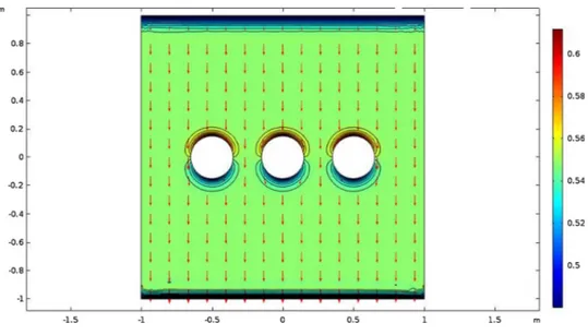
For numerical work, the above systems are often used spherical magnetic flux density. Spherical magnetic ϕ(s) Landau Lifshitz flux is usually derived using the properties of the divergence-free nature of the magnetic field along with the definition of the spherical magnetic flux density. To obtain the visualization of the evolved systems of the magnetic ϕ(s) flux m_ℱ

ϕ(s)we use the basic numerical

algorithms to solve the above equations at Matlab and Comsol software. This approach presents the results of the magnetic ϕ(s) flux

m_ℱ

ϕ(s)on the spherical magnetic flux density and magnetic field of an ideal conductor at minimum density are illustrated in Fig. 3. 5. Application to fractional calculus

In this section, the connection between the Laplacian-like non-linear equation the celebrated Heisenberg Landau Lifshitz model flow is investigated in the spherical magnetic flux density and spherical flow lines. For magnetic ϕ(α)flux surface, we have already induced solitonic equations that are associated with curves of geometric quantities. If one considers the appropriate limiting and scaling process then a basic geometric derivation admits the following reciprocal transformation

∂θ_ε₍_σ_,_t) ∂tθ − ω ∂2_ε₍_σ_,_t) ∂σ2 +ε(σ,t) 2 χ=0, (1) where ∂θ

∂tθ is the conformable derivative operator; ω and χ are real valued constants. In [38]; scientists studied conformable type of

fractional derivative in 2014 as a new definition of local fractional operator. It’s very easier to work with this fractional derivative. Recently, several studies have been done relatedto conformable type of fractional calculations [39,40].

The definition of conformable fractional derivative of order θ ∈ (0, 1) defined as the following expression [38],

tDθf (t) = lim ε→0

f (t +εt1− θ_{) −} _{f (t)}

ε , f : (0, ∞) → ℝ. (2)

Some of the features of conformable fractional derivative as follows [38]. a)tDθtα=αtα−θ, ∀θ ∈ ℝ, b)tDθ(fg) = ftDθg + gtDθf , c)tDθ(fog) = t1− θg ′ (t)f′(g(t)), d)tDθ( f g) = gtDθf − ftDθg g2 .

•Suppose the traveling wave variable: ε(σ,t) = u(ϕ), ϕ =σ− vt

θ

θ. (3)

Then, from Eq. (5.3), Eq. (5.1) is turn to an ordinary differential equation for ωu′′₍_{ϕ) + vu}′

(11)

Consider the solutions of Eq. (5.4) can write as a series expansion solution as follows,

u(ϕ) = A0+A1G(ϕ) + A2G−1(ϕ) + B1G(ϕ)2+B2G−2(ϕ), (5) where A0,A₁,A₂,B₁,B₂are functions to be determined later and G(ϕ) satisfies the fractional Riccati equation as follows:

G′(ϕ) = ξ + G2₍_ϕ), ₍₆₎

where ξ is an arbitrary constants.

•N is obtained with the aid of balance between the highest order derivatives and the nonlinear terms in Eq.(5.4). A few special solutions of Eq. (5.5) are given by;

1) When ξ < 0, G1(ϕ) = − √̅̅̅̅̅̅− ξtanh(√̅̅̅̅̅̅− ξϕ), (7) G2(ϕ) = − ̅̅̅̅̅̅ − ξ √ coth(√̅̅̅̅̅̅− ξϕ), 2) When ξ > 0, G3(ϕ) = √̅̅̅ξtan(√̅̅̅ξϕ), (8) G4(ϕ) = ̅̅̅ ξ √ cot(√̅̅̅ξϕ), 3) When ξ = 0,ρ =const., G5(ϕ) = − 1 ϕ +ρ. (9)

Now, replacing (5.5) and (5.6) into (5.4), by equating the all coefficients of G(ϕ), we can solve equations. Then we obtain the following some functions:

A0= − v2 50ωχ+ 4ωσ χ ,A1= 6v 5χ,A2= v3₊_100v_ω2_σ 250ω2_χ , (10) B1= 6ω χ,B2= − 7v4₊₂₀₀₀_ω4_σ2 5000ω3_χ .

Then by using ξ = 1, G(ϕ) =√ tan( ̅̅̅ξ̅̅̅ξ √ϕ),we obtain u(ϕ) = − v 2 50ωχ+ 4ωσ χ + 6v 5χ ̅̅̅ ξ √ tan(√̅̅̅ξϕ) +v 3₊_100v_ω2_σ 250ω2_χ ( ̅̅̅ ξ √ tan(√̅̅̅ξϕ))−1 +6ω χ ( ̅̅̅ ξ √ tan(√̅̅̅ξϕ))2− 7v 4₊₂₀₀₀_ω4_σ2 5000ω3_χ ( ̅̅̅ ξ √ tan(√̅̅̅ξϕ))−2. From here, ε(σ,t) = − v 2 50ωχ+ 4ωσ χ + 6v 5χ ̅̅̅ ξ √ tan(√̅̅̅ξ(σ− vt θ θ)) + v3₊_100v_ω2_σ 250ω2_χ ( ̅̅̅ ξ √ tan(σ− vt θ θ)) −1 ₍₁₁₎ +6ω(√̅̅̅ξtan(√̅̅̅ξ(σ− vt θ )))2− 7v 4₊₂₀₀₀_ω4_σ2 (√̅̅̅ξtan(√̅̅̅ξ(σ− vt θ )))−2_.

(12)

By using ξ = − 1, G(ϕ) = − √̅̅̅̅̅̅− ξtanh(√̅̅̅̅̅̅− ξϕ),we obtain u(ϕ) = − v 2 50ωχ+ 4ωσ χ + 6v 5χ(− ̅̅̅̅̅̅ − ξ √ tanh(√̅̅̅̅̅̅− ξϕ)) +v 3₊_100v_ω2_σ 250ω2_χ (− ̅̅̅̅̅̅ − ξ √ tanh(√̅̅̅̅̅̅− ξϕ))−1 +6ω χ (− ̅̅̅̅̅̅ − ξ √ tanh(√̅̅̅̅̅̅− ξϕ))2− 7v 4₊₂₀₀₀_ω4_σ2 5000ω3_χ (− ̅̅̅̅̅̅ − ξ √ tanh(√̅̅̅̅̅̅− ξϕ))−2, From here, ε(σ,t) = − v 2 50ωχ+ 4ωσ χ + 6v 5χ(− ̅̅̅̅̅̅ − ξ √ tanh(√̅̅̅̅̅̅− ξ(σ− vt θ θ))) + v3₊_100v_ω2_σ 250ω2_χ (− ̅̅̅̅̅̅ − ξ √ tanh(√̅̅̅̅̅̅− ξ(σ− vt θ θ))) −1 +6ω χ(− ̅̅̅̅̅̅ − ξ √ tanh(√̅̅̅̅̅̅− ξ(σ− vt θ θ))) 2₋ 7v4+2000ω4σ2 5000ω3_χ (− ̅̅̅̅̅̅ − ξ √ tanh(√̅̅̅̅̅̅− ξ(σ− vt θ θ))) −2_. ₍₁₂₎ Figs. 4–6 6. Conclusion

Flows theory an important part of geometric optic, optical physics, and magnetic motion, [41–51]. In our paper, we obtain some optical conditions of spherical Sα-magnetic Lorentz flux by using directional spherical fields. Moreover, we determine spherical magnetic Lorentz flux for spherical vector fields. Also, we give new construction for spherical curvatures of spherical Sα-magnetic particle flows by considering Heisenberg spherical Landau Lifshitz model. Finally, magnetic flux surface is demonstrated in a static and uniform magnetic surface by using the analytical and numerical results with Heisenberg spherical Landau Lifshitz model.

In our future work beneath this kind of idea, we offer to review spherical magnetic Lorentz flux of St-magnetic particles in de Sitter space. Another purpose of the future studies will be explore the unified formulations of the systems composed of arbitrary dyons, magnetic and electric charges of manifolds with magnetic flux lines.

Declaration of Competing Interest

The authors report no declarations of interest.

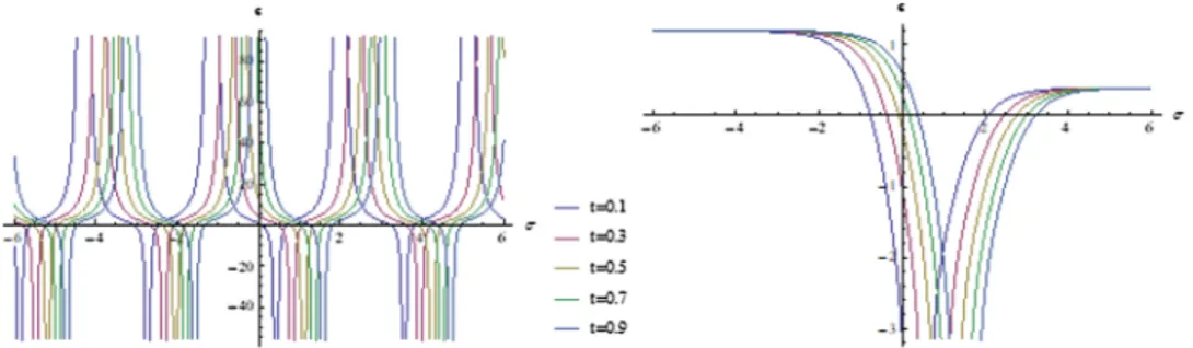
Fig. 5. The 2D graphic for ε(σ,t) analytical solutions of Eq. (5.1) for different value of t. (ω=1,χ=2,v = 1,θ = 0.6). (a) for solution (5.11), (b) for

solution (5.12).

Fig. 6. The 2D graphic for ε(σ,t) analytical solutions of the Eq. (5.1) for different value of θ. (ω=1,χ=2,v = 1,σ =2). (a) for solution (5.11), (b)

(13)

References

[1] R. Gilmore, Length and curvature in the geometry of thermodynamics, Phys. Rev. A 30 (4) (1984) 1994. [2] B.M. Barbashov, V. Nesterenko, Introduction to the Relativistic String Theory, World Scientific, 1990. [3] V. De Sabbata, C. Sivaram, Spin and Torsion in Gravitation, World Scientific, 1994.

[4] W.K. Schief, C. Rogers, The Da Rios system under a geometric constraint: the Gilbarg problem, J. Geometry Phys. 54 (3) (2005) 286–300. [5] R.G. Littlejohn, Variational principles of guiding centre motion, J. Plasma Phys. 29 (1) (1983) 111–125.

[6] M. Kleman, Developable domains in hexagonal liquid crystals, J. Physique 41 (7) (1980) 737–745.

[7] T. K¨orpinar, R.C. Demırkol, Electromagnetic curves of the linearly polarized light wave along an optical fiber in a 3D Riemannian manifold with Bishop equations, Optik 200 (2020) 163334.

[8] T. Korpinar, R.C. Demirkol, Frictional magnetic curves in 3D Riemannian manifolds, Int. J. Geometr. Methods Modern Phys. 15 (02) (2018) 1850020. [9] T. K¨orpınar, R.C. Demirkol, Gravitational magnetic curves on 3D Riemannian manifolds, Int. J. Geometr. Methods Modern Phys. 15 (11) (2018) 1850184. [10]A. Kazan, H.B. Karadag, Magnetic pseudo null and magnetic null curves in Minkowski 3-space, Int. Math. Forum 123 (2017) 119–132.

[11]S¸. Güvenç, C. ¨Ozgür, On slant magnetic curves in S-manifolds, J. Nonlin. Math. Phys. 26 (4) (2019) 536–554. [12]J.L. Cabrerizo, Magnetic fields in 2D and 3D sphere, J. Nonlin. Math. Phys. 20 (3) (2013) 440–450.

[13]J. Sun, Singularity properties of killing magnetic curves in Minkowski 3-space, Int. J. Geometr. Methods Modern Phys. 16 (08) (2019) 1950123.

[14]T. K¨orpınar, R.C. Demirkol, Z. K¨orpınar, V. Asil, Maxwellian evolution equations along the uniform optical fiber in Minkowski space, Revista Mexicana de Física 66 (4) (2020) 431–439.

[15]T. K¨orpınar, R.C. Demirkol, Z. K¨orpınar, V. Asil, Maxwellian evolution equations along the uniform optical fiber in Minkowski space, Optik 217 (2020) 164561. [16] R.L. Ricca, 2005. Inflexional disequilibrium of magnetic flux-tubes, Fluid Dynamics Research 36(4-6), 319.

[17]R.L. Ricca, Evolution and inflexional instability of twisted magnetic flux tubes, Solar Phys. 172 (1-2) (1997) 241–248. [18]L.C. Garcia de Andrade, Non-Riemannian geometry of twisted flux tubes, Brazil. J. Phys. 36 (4A) (2006) 1290–1295.

[19]L.C. Garcia de Andrade, Riemannian geometry of twisted magnetic flux tubes in almost helical plasma flows, Phys. Plasmas 13 (2) (2006), 022309-022309. [20]L.C. Garcia de Andrade, Vortex filaments in MHD, Phys. Scr. 73 (5) (2006) 484.

[21]M. Yenero˘glu, T. K¨orpinar, A new construction of Fermi–Walker derivative by focal curves according to modified frame, J. Adv. Phys. 7 (2) (2018) 292–294. [22]T. K¨orpinar, R.C. Demirkol, V. Asil, The motion of a relativistic charged particle in a homogeneous electromagnetic field in De-Sitter space, Revista Mexicana de

Fisica 64 (2018) 176–180.

[23]Y. Ünlütürk, T. K¨orpınar, M. Çimdiker, On k-type pseudo null slant helices due to the Bishop frame in Minkowski 3-space E3

1, AIMS Math. 5 (1) (2020) 286–299.

[24]T. K¨orpınar, Y. Ünlütürk, An approach to energy and elastic for curves with extended Darboux frame in Minkowski space, AIMS Math. 5 (2) (2020) 1025–1034. [25]M. Yenero˘glu, On new characterization of inextensible flows of space-like curves in de Sitter space, Open Math. 14 (2016) 946–954.

[26]T. K¨orpinar, A new optical Heisenberg ferromagnetic model for optical directional velocity magnetic flows with geometric phase, Indian J. Phys. 94 (9) (2020) 1409–1421.

[27]R. Balakrishnan, A.R. Bishop, R. Dandoloff, Anholonomy of a moving space curve and applications to classical magnetic chains, Phys. Rev. B 47 (6) (1993) 3108. [28]M. Barros, A. Ferr´andez, P. Lucas, M. Merono, Hopf cylinders, B-scrolls and solitons of the Betchov-Da Rios equation in the 3-dimensional anti-De Sitter space,

CR Acad. Sci. Paris, S´erie I 321 (1995) 505–509.

[29]M. Barros, A. Ferr´andez, P. Lucas, M.A. Mero no, Solutions of the Betchov-Da Rios soliton equation: a Lorentzian approach, J. Geometry Phys. 31 (2-3) (1999) 217–228.

[30] Arroyo, J., Garay, Ó. J., Pámpano, Á. 2017. Binormal motion of curves with constant torsion in 3-spaces, Advances in Mathematical Physics 2017. [31]T. Körpınar, R.C. Demirkol, Z. Körpınar, Soliton propagation of electromagnetic field vectors of polarized light ray traveling along with coiled optical fiber on

the unit 2-sphere S2_{, Rev. Mex. Fis. 65 (6) (2019) 626–633}_.

[32]T. K¨orpınar, R.C. Demirkol, Z. K¨orpınar, Soliton propagation of electromagnetic field vectors of polarized light ray traveling in a coiled optical fiber in Minkowski space with Bishop equations, Eur. Phys. J. D 73 (9) (2019) 203.

[33]T. K¨orpınar, R.C. Demirkol, Z. K¨orpınar, Soliton propagation of electromagnetic field vectors of polarized light ray traveling in a coiled optical fiber in the ordinary space, Int. J. Geometric Methods Modern Phys. 16 (8) (2019) 1950117.

[34]R. Balakrishnan, A.R. Bishop, R. Dandoloff, Geometric phase in the classical continuous antiferromagnetic Heisenberg spin chain, Phys. Rev. Lett. 64 (18) (1990) 2107.

[35]K.Y. Bliokh, Geometrodynamics of polarized light: Berry phase and spin Hall effect in a gradient-index medium, J. Opt. A: Pure Appl. Opt. 11 (9) (2009) 094009. [36]K.Y. Bliokh, A. Niv, V. Kleiner, E. Hasman, Geometrodynamics of spinning light, Nat. Photon. 2 (12) (2008) 748.

[37]F. Wassmann, A. Ankiewicz, Berry’s phase analysis of polarization rotation in helicoidal fibers, Appl. Opt. 37 (18) (1998) 3902–3911. [38]R. Khalil, M. Al Horani, A. Yousef, M. Sababheh, A new definition of fractional derivative, J. Comput. Appl. Math. 264 (2014) 65.

[39]Z. Korpinar, Some analytical solutions by mapping methods for nonlinear conformable time-fractional Phi-4 equation, Thermal Sci. 23 (6) (2019) 1815. [40]Z. Korpinar, F. Tchier, M. Inc, L. Ragoub, M. Bayram, New solutions of the fractional Boussinesq-like equations by means of conformable derivatives, Results

Phys. 13 (2019) 1023392.

[41]Z. K¨orpınar, M. ˙Inç, On the Biswas–Milovic model with power law nonlinearity, J. Adv. Phys. 7 (2) (2018) 239.

[42]T. K¨orpinar, S. Bas¸, A new approach for inextensible flows of binormal spherical indicatrices of magnetic curves, Int. J. Geom. Methods Mod. Phys. 16 (2) (2019) 1950020.

[43]G.U. Kaymanli, M. Dede, C. Ekici, Directional spherical indicatrices of timelike space curve, Int. J. Geometr. Methods Modern Phys. 17 (11) (2020) 2030004. [44]T. K¨orpinar, Tangent bimagnetic curves in terms of inextensible flows in space, Int. J. Geom. Methods Mod. Phys. 16 (2) (2019) 1950018.

[45]T. K¨orpinar, Optical directional binormal magnetic flows with geometric phase: Heisenberg ferromagnetic model, Optik 219 (2020) 165134.

[46]T. K¨orpınar, R.C. Demirkol, Electromagnetic curves of the linearly polarized light wave along an optical fiber in a 3D semi-Riemannian manifold, J. Modern Opt. 66 (8) (2019) 857–867.

[47]T. K¨orpinar, A new version of energy for involute of slant helix with bending energy in the Lie groups, Acta Sci. Technol. 41 (e36569) (2019) 1–8. [48]T. K¨orpinar, A new version of normal magnetic force particles in 3D Heisenberg Space, Adv. Appl. Clifford Algebras 28 (2018) 83.

[49]T. Körpinar, On T-magnetic biharmonic particles with energy and angle in the three dimensional Heisenberg Group H, Adv. Appl. Clifford Algebras (2018) 28. [50] T. Körpınar, R.C. Demirkol, Z. Körpınar, 2021. Binormal Schrodinger System of Wave Propagation Field of Light Radiate in the Normal Direction with q-HATM

Approach, Optik - International Journal for Light and Electron Optics https://doi.org/10.1016/j.ijleo.2021.166444.

[51]T. K¨orpınar, R.C. Demirkol, Curvature and torsion dependent energy of elastica and nonelastica for a lightlike curve in the Minkowski Space, Ukrainian Math. J. 72 (2021) 1267–1279.