Computer Information Sciences
Finding Best Performing Solution Algorithm for the QAP
Master Thesis
Burcu Müzeyyen Kıyıcığı
200791001
Advisor
Assoc. Prof. Ekrem Duman
June 2010
Istanbul
I would like to thank my advisor Assoc. Prof. Ekrem Duman for his direction and
guidance. Assoc. Prof. Ekrem Duman’s and Assist. Prof. Dr. Ali Fuat Alkaya’s
recommendations and suggestions have been invaluable for my master thesis. Also I would
like to thank TUBITAK for supporting my master thesis through the project 108M198.
Istanbul, June 2010 Burcu Müzeyyen KIYICIĞI
The quadratic assignment problem (QAP) o f NP-Hard problems class is known as one of
the hardest combinatorial optimization problems. In this thesis, a search is performed on
the metaheuristics that have recently found widespread application in order to identify a
heuristic procedure that performs well with the QAP. Algorithms which reflect
implementations o f Simulated Annealing, Genetic Algorithm, Scatter Search and Grasp -
type metaheuristics are tested and using real test problems these algorithms are compared.
Same set o f algorithms are tested on general QAP problems and observation to identify
successful algorithms is made. To conclude the best performing heuristic is not easy to
name due to the fact that the performance of a heuristic depends on the context of the
problem, which determines the structure and relationships o f problem parameters.
Karesel atama problemi (KAP), NP-Zor sınıfına ait olup en zor kombinasyonel
optimizasyon problemlerinden birisi olarak bilinir. Bu tez çalışmasında, KAP ile
kullanılabilen en uygun sezgisel yöntemi tanımlayabilmek için yaygınca kullanılan meta
sezgisel uygulamalar incelenmiş ayrıca Benzetimli tavlama, Genetik algoritma, Dağınık
arama ve Açgözlü rassallaştırılmış uyarlamalı arama yordamı algoritmaları ile test edilmiş
ve gerçek test problemleri ile karşılaştırılmıştır. Bunların dışında, aynı algoritmalar genel
KAP problemlerinde test edilmiş ve hangi algoritmaların başarılı olduğu gözlemlenmiştir.
Bu gözlemlere dayanarak özetlemek gerekirse, sezgisel algoritmaların performansı
problemin içeriğine bağlı olduğu için ve bu da problemin yapısı ve parametreleri ile ilişkili
olduğundan en iyi sezgisel algoritmayı tespit etmek oldukça güçtür.
Page ACKNOWLEDGMENTS ...i A B ST R A C T ... ii ÖZET ... iii TABLE OF C O N T E N T S... iv LIST OF FIGURES ... vi
LIST OF TA BLES... vii
SYMBOLS... viii
1. INTRODUCTION ... 1
1.1. The Quadratic Assignment Problem (Q A P )... 1
1.2. Algorithms for the Q A P... 3
1.3. M ethodology...6
1.4. Outline o f Study... 6
2. ALGORITHMS IM PLEM ENTED... 7
2.1. Simulated Annealing...7
2.1.1. Parameters T u n e d ... 9
2.2. Genetic A lgorithm ... 10
2.2.1. Parameters T u n e d ... 16
2.3. Scatter Search Algorithm ... 17
2.3.1. Parameters T u n e d ... 22
2.4. Grasp A lgorithm ... 23
2.4.1. Parameters T u n e d ... 25
3. EXPERIMENTAL R E S U L T S ... 27
3.1. Simulated Annealing - Test R esults... 28
3.2. Genetic Algorithm - Test Results...30
3.3. Scatter Search - Test R esults... 32
3.4. Grasp - Test R esu lts... 34
4. COMPARISON OF ALGORITHM S... 36
4.1. Summary... 38
5. REFEREN CES...40
Figure-2.2.1: Pseudocode - G A ... 15
Figure-2.3.1: Pseudocode - SS Algorithm - S P R ... 20
Figure-2.3.2: Pseudocode - SS Algorithm - SL C ... 21
Figure-2.4.1: Pseudocode - G X ...24
Table 2.2.1 : GA- parameters used ...14
Table 2.2.1.1 : Parameter settings o f G A ... 17
Table 2.3.1 : Parameter settings o f S S ... 23
Table 2.4.1 : Parameter settings o f G X ...26
Table 3.1 : The number o f components in each problem s...27
Table 3.2 : The context o f test problem (PS11AK08-9)... 27
Table 3.1.1 : SA - best average and best solution of problems...28
Table 3.1.2 : SA - test results and parameters u se d ... 29
Table 3.2.1 : GA- best average and best solution of problems (G 1-G 12)... 30
Table 3.2.2 : GA- test results and parameters u s e d ...31
Table 3.3.1 : SS - best average and best solution o f problems (S1 - S14)... 32
Table 3.3.2 : SS- test results and parameters u sed ...33
Table 3.4.1 : GX - best average and best solution o f problems (R1-R10)... 34
Table 3.4.2 : GX- test results and parameters u s e d ... 35
Table 4.1.1 : Best average of algorithm s... 36
Table 4.1.2 : Best solution of algorithms... 37
Table 4.2.1 : Best average of each problem in algorithm s... 37
Table 4.2.2 : Best solution of each problem in algorithm s... 38
Table 6.1 : Simulated Annealing - full test results... 44
Table 6.2 : Genetic Algorithm - full test results... 46
Table 6.3 : Scatter Search - full test results... 48
Table 6.4 : Grasp - full test results...51
KAP - Karesel Atama Problemi SA - Simulated Annealing GA - Genetic Algorithm SS - Scatter Search GX - Grasp viii
1. IN T R O D U C TIO N
The quadratic assignment problem (QAP), which is one o f the hardest combinatorial
optimization problems, is in the class o f NP-Hard problems (Duman and Or, 2007). Many
applications in several areas such as operational research, parallel and distributed
computing, and combinatorial data analysis can be modelled by the QAP. Moreover, the
QAP can be used to formulate other combinatorial optimization problems such as maximal
clique, the travelling salesman problem, graph partitioning and isomorphism. The efficient
heuristic methods known as Simulated Annealing, Genetic Algorithm, Scatter Search and
Grasp can find a solution for the QAP. The goal o f the thesis is to do a comparison of these methods from a QAP perspective.
1.1. The Q u a d ratic A ssignm ent P roblem (QAP)
Matching n facilities with n locations causes a cost because o f the interactions between the
facilities. The main purpose o f the quadratic assignment problem (QAP) is to minimize the
total weighted cost. The following is a representation o f the QAP.
n n n n min I I Z Z c A V , (1.1.1) i =1 j =1 k= 1 1=1 n
IX =1’
k = \ , . . . , n i =1 nI X =1>
i = \ — ,n k =1 x ik e Gjl , j i,kEquation 1.1.1: QAP formulation. (Koopmans and Beckmann, 1957)
Where xik = 1 means that k is assigned to i, dkl is a matrix o f flow o f items to be
transported between facilities and also cij is a matrix containing the distances or costs of
transporting a single item between any two locations and also finding an assignment vector
which minimizes the total transportation costs given by the sum o f the product o f the flow
The QAP was first conceived as a mathematical model by Koopmans and Beckmann
(1957) for economic activities, but it has been used in many different areas. It was applied
in minimizing the total amount o f connections between components in a backboard wiring
by Steinberg (1961), in economic problems by Heffley (1972, 1980), in scheduling
problems by Geoffrion and Graves (1976), in defining the best design for typewriter
keyboards and control panels by Pollatschek et al (1976), in archeology by Krarup and
Pruzan (1978), in parallel and distributed computing by Bokhari (1987), in statistical
analysis by Hubert (1987), in the analysis o f reaction chemistry by Forsberg et al (1994), in
numerical analysis by Brusco and Stahl (2000). However, the most regarded application
where QAP is used is the facilities layout problem. Dickey and Hopkins (1972) modelled
the assignment o f buildings in a University campus with QAP. Elshafei (1977) carried out
a hospital planning and Bos (1993) used the QAP for similar reasons in planning o f forest parks. A formulation o f the facility layout design problem was done by Benjaafar (2002) to
minimize work-in-process (WIP).
In spite o f the fact that the QAP has been regarded as a popular model for facility layout
problem, it is used in a wide range o f area including chemistry, transportation, information
retrieval, scheduling, statistical data analysis, parallel and distributed computing. As all the
incoming and departing flights at an airport need to be directed to gates, assigning flights to gates can be modelled with QAP (Haghani and Chen, 1998). Allocation is an important
logistic application o f the QAP. Assigning rooms to persons by caring the undesirable
neighbourhood constraints was formulated as a QAP by Ciriani, Pisanti, and Bernasconi
(2004). To minimize the container rehandling operations at a shipyard, a generalization of
the QAP was applied (Cordeau et al., 2005). Another location analysis problem which can
be formulated as QAP is the parallel computing and networking (Gutjahr, Hitz, and
Mueck, 1997; Siu and Chang, 2002). We consult Cela (1998) and Loiola et al (2007) to
have in detailed knowledge about these and other applications o f the QAP. Numerous other
well-known combinatorial optimization problems such as the travelling salesman problem,
the bin-packing problem, the maximum clique problem, the linear ordering problem and
the graph-partitioning problem can be formulated as the QAP. It is easy to see that QAP
has a variety of usage in many fields including transportation, manufacturing, logistics,
The QAP is known as a very complex problem since there is no algorithm to solve QAP
instances with medium or large number of inputs. (Anstreicher et al., 2002) is one of the
most successful approaches for the QAP implemented on a large grid which obtains
optimal solutions for problems o f size 30.
Many approaches have been implemented to QAP to overcome its solution difficulty.
1.2. A lgorithm s fo r the QAP
Seven of basic categories o f approaches o f QAP investigated in our research are Simulated
annealing, Genetic algorithm, Scatter search, Grasp, Ant colony optimization, Tabu search
and Variable neighbourhood search.
First algorithm we investigate is Simulated annealing which is an algorithm that feats the
analogy which is made by solutions of combinatorial optimization problem to states o f the
physical system and cost related solutions to these states energies between optimization
algorithms and statistical mechanics (Kirkpatrick et al., 1983).
Let Ei and Ei+1 be energy states to two neighbour solutions.
AE = Ei+1 - Ei. (1.2.1)
Equation 1.2.1: Deterioration formula (Duman and Or, 2007).
These are the possible states which can occur: If AE is less than zero, continually energy
reduction occurs which means problem cost function is reduced and the new allocation
may be accepted. If AE is equal to zero, there is no change in the energy state and also
problem cost function is not changed. If AE is more than zero, problem cost function is
increased as well as the energy; to avoid poor local minima to come together the values
One o f the first applications o f Simulated Annealing is proposed by Burkard and Rendl
(1984) which is followed by Wilhelm and Ward (1987) adding new equilibrium
components, other approach introduced by Abreu et al (1999), number o f inversions o f the
problem solution and cost were reduced. Other approaches for simulated annealing applied
to QAP are as follows: Bos (1993), Yip and Pao (1994), Burkard et al (1995), Peng et al
(1996), Tian et al (1996, 1999), Mavridou and Pardalos (1997), Chiang and Chiang (1998),
Misevicius (2000, 2003), Tsuchiya et al (2001), Siu and Chang (2002), Baykasoglu (2004),
Duman and Or (2007).
Natural selection and adaptation are simulated by using Genetic Algorithms which
generates a new solution by applying genetic operations on populations o f initial solutions,
cost is worked out and best solutions should be selected. More information about genetic
algorithms can be found in: Brown et al (1989), Bui and Moon (1994), Tate and Smith
(1995), Mavridou and Pardalos (1997), Kochhar et al (1998), Gong et al (1999). Other
approaches for the genetic algorithms applied to QAP are Drezner and Marcoulides (2003),
El-Baz (2004) and W ang and Okazaki (2005).
Glover (1977) introduced a Scatter Search method based on a study on linear programming
problems. Therefore, method would take linear combinations o f solution and generate new solution vectors in successive generations. Furthermore, metaheuristic is combination of
initial phase where group of good solutions is referenced and evolutionary phase where
new solutions are generated by using those references. Once the best generated solution is
selected, it would be moved to reference set and then it will continue until a stop criterion
is satisfied. Scatter search applications to the QAP can be found in Cung et al (1997). The
publications o f Scatter search are much less than other algorithms (Loiola et al., 2007).
Several researchers as follows applied the technique called (GRASP) which obtains
approximate solution for the problem Li et al (1994), Feo and Resende (1995), Resende et
al (1996), Fleurent and Glover (1999), Ahuja et al (2000), Pitsoulis et al (2001), Rangel et
al (2000) and Oliveira et al (2004) built a GRASP using the path-relinking strategy, which
Ant colony optimization (ACO) is a class o f distributed algorithms which hold the
definitions o f properties o f agents called ants. It is based on the idea how ants are able to
make their way from colony to a food source. Ants work together in an ordinary activity to
solve the problem. The main property o f this method is these agents generate a synergetic
effect since they work together and interact each other and the quality o f solutions found
increases. Numerical results for the QAP are presented in Maniezzo and Colorni (1995,
1999), Colorni et al (1996), Dorigo et al (1996) and Gambardella et al (1999) indicate that
ant colony method generate few good solutions mainly close to each other therefore it is
stated as a competitive metaheuristic.
Glover (1989) introduced a local search algorithm called Tabu Search to overcome integer
programming problems with quality solutions where search process has list of best
solutions with a priority value or an aspiration criterion, history o f search process. Tabu list
information and their priorities were used for new allocations in the neighbourhood to be
accepted or rejected this way neighbourhood diversification and intensification was
provided. Adaptations o f this mechanism to QAP can be found in Skorin (1990, 1994),
Taillard (1991), Bland and Dawson (1991), Rogger et al (1992), Chakrapani and Skorin-
QAPov (1993), Misevicius (2003, 2005) and Drezner (2005). This mechanism was
dependent on tabu list and how it is managed but it was shown that very good performance
for QAP Taillard (1991) and Battiti and Tecchiolli (1994). Genetic algorithm and tabu
search were compared by Taillard (1995) when they are applied to QAP.
Variable neighbourhood search (VNS) was proposed by Mladenovic and Hansen (1997).
This search is systematic movement between set of neighbourhoods where there are a
number o f change rules defined that are used when there is no better solution in the current
neighbourhood. VNS was applied to large combinatorial problems in Taillard and
Gambardella (1999), three VNS strategies are introduced for the QAP.
There are other combined algorithms for the QAP. A combination o f simulated annealing
and genetic algorithm is presented by Bolte and Thonemann (1996). A combination o f tabu
Dawson (1994), Chiang and Chiang (1998) and Misevicius (2001, 2004). Tabu search with
a neural network was used by Talbi et al (1998) and Hasegawa et al (2002). And also tabu
search and simulated annealing with fuzzy logic was used by Youssef et al (2003). A
combination o f genetic algorithm and tabu search with some hybrid algorithms is presented
by Fleurent and Ferland (1994), Drezner (2003).
1.3. M ethodology
In this research, a search is performed among those meta heuristic that have recently
discovered widespread application which identifies a heuristic procedure that fits well with
QAP. Specific algorithms reflecting implementations o f Simulated Annealing, Genetic
Algorithm, Scatter Search and Grasp - type meta heuristic were tested and compared using
real data. The same set o f algorithms is tested on common QAP problems as well. A
sample Java application using Eclipse programming platform is made in order to compare
the performance o f meta-heuristics algorithms. There are eleven problems defined in
(Duman and Or, 2007) eight o f which we could obtain. This is the reason why only eight
problems are tested. Deciding the best performing heuristic algorithm is complicated due
to the fact that performance o f a heuristic algorithm depends on the context o f the problem
which is determined by the structure and relationship o f problem parameters.
1.4. O utline of Study
In the second part, we describe the formulation o f the QAP and give information about
algorithms o f the QAP. In the third part, Simulated annealing, Genetic algorithm, Scatter
search and Grasp are described with their parameters. In the fourth part, these algorithms’
test results are presented. In the fifth part, find the best performing heuristic is tried to be
2. A L G O R IT H M S IM PL E M E N T E D
This work is an experimental one. A sample Java application using Eclipse programming
platform is made in order to compare the performance o f meta-heuristics algorithms. These
methods are Simulated annealing, Genetic algorithm, Scatter search and Grasp. (Duman
and Or, 2007)’s literature problems are used for testing the methods. W e present the best
solution obtained by each method.
2.1. Sim ulated A nnealing
In order to avoid local minima Simulated Annealing is used, it is one o f the first algorithms
which had a clear strategy that allowed worse quality solutions than the current solution to
move, first an initial solution should be created randomly or heuristically, temperature
parameter T should be initialized then N(s) is generated using solution s’ at each value and
current solution is accepted to be dependent on f(s), f(s’) and T. Also s’ replaces s if f(s’) <
f(s) or, in case f(s’) > f(s), with a probability which is a function o f T and f(s’)-f(s).
Boltzmann distribution shows the probability as follows / O / c
T
e (Blum and Roli, 2003).
Having T in high values at the beginning and exchanges in pairs helps to avoid a local
optimum to be trapped. T approaches zero and iterations are less than maximum iteration
number (Noi) when pair wise exchanges keep happening. Simulated annealing
A lgorithm BT 0. bs = cs.random() 1. while(T>0&&totalR<Noi){ 2. for(j=0;j<R;j++){ 3. ns=cs.neighbour(); 4. delta=ns.getCost()-bs.getCost(); 5. if(ns.getCost()<cs.getCost()){cs=ns;} 6. else if(Math.random()<Math.exp(-Math.abs(delta)/T)){cs=ns;} 7. if(ns.getCost()<bs.getCost()){bs=ns;} } 8. T/=a; 9. R*=b; 10. totalR+=R; }______________________________________________ Figure-2.1.1: Pseudocode SA
The variables in simulated annealing implementations are: initial temperature (T),
temperature decrease ratio (a), number of iterations at each temperature setting (R), increase ratio in iteration number at each setting (b), maximum iteration number (Noi),
current solution (cs), neighbour solution (ns) and best solution (bs). The acceptance
probability is set to e(-A/T), where A is the deterioration level. Neighbour solution is
achieved by pair wise exchange in the current solution.
In Figure-2.1.1, until T is bigger than zero or total R is less than maximum iteration
number (Noi), the process continues in line (1-10). Until ‘j ’ is less than ‘R ’, the process
continues in line (2-7). In the first line (0), current solution (cs) is chosen randomly and
‘cs’ is assigned to ‘bs’. The random neighbour (ns) is chosen by current solution (cs) in
line (3). AEns and AEbs are two energy successive states, corresponding to two neighbour
solutions and calculate AE to the difference between AEns and AEbs in line (4). If the cost
function of neighbour solution (ns) is less than the cost function of current solution (cs),
‘ns’ is assigned to ‘cs’ in line (5). Otherwise, If random(0, 1) is less than exp(AE /T), ‘ns’
is assigned to ‘cs’ in line (6). If the cost function of neighbour solution (ns) is less than the
cost function of best solution (bs), ‘ns’ is assigned to ‘bs’ in line (7). T is decreased by T/a
2.1.1. P aram eters T uned
There are some parameters as follows:
i. Initial temperature (T) is set to either 100 (accepting 10 percent worse solutions has
a probability o f 0.05) or 1000 (accepting 10 percent worse solutions has a
probability o f 0.75) (Duman and Or, 2007).
ii. Temperature decrease ratio (a) is set to either 1.1 or 1.5 (Duman and Or, 2007).
iii. Number o f iterations at each temperature setting (R) is set to either 5 or 25 (Duman
and Or, 2007).
iv. Increase ratio in iteration number at each setting (b) is set to either 1.1 or 1.5
(Duman and Or, 2007).
3 3
v. Iteration number (Noi) is set to either N3 or N3/ 3 (Duman and Or, 2007).
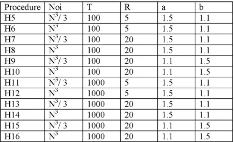
Depending on different combinations o f parameters 12 different simulated annealing
heuristics are established (Table 2.1.1).
Table 2.1.1 Parameter settings o f SA.
Procedure Noi T R a b H5 N 3/ 3 100 5 1.5 1.1 H6 N 3 100 5 1.5 1.1 H7 N 3/ 3 100 20 1.5 1.1 H8 N 3 100 20 1.5 1.1 H9 N 3/ 3 100 20 1.1 1.5 H10 N 3 100 20 1.1 1.5 H11 N 3/ 3 1000 5 1.5 1.1 H12 N 3 1000 5 1.5 1.1 H13 N 3/ 3 1000 20 1.5 1.1 H14 N 3 1000 20 1.5 1.1 H15 N 3/ 3 1000 20 1.1 1.5 H16 N 3 1000 20 1.1 1.5
Parameters used are the same as (Duman and Or, 2007). 12 heuristic algorithms were
tested on eight test problems. The results are given in (3.1).
2.2. G enetic A lgorithm
Genetic algorithms are based on natural evolution principles (Holland, 1990) and search
number o f solutions which are generated randomly or heuristically. To produce offspring
(new individuals o f the next generation). The population is developed by genetic operators
like mutation which provides random modifications o f the chromosome and diversity and
crossover which creates new offspring by combining two parents. The parents (individuals
from the current generation) are chosen depending on their survival, the offspring is
become o f the values which survived more. (Beasley et al., 1993).
The fitness function which shows the quality o f an individual should determine the value
o f an invidual’s performance in the current population. The fitness value which is
dependent on the objective value is changed by the normalization. The equation is as
follows:
fitnessi = (fi - fm in ) \ (fm ax - fm in ) (2.2.1) Equation 2.2.1: Fitness function (Omatu and Yuan, 2000).
Where
f : The objective value o f individual i.
fm in : The minimum objective value o f current population. fm ax : The maximum objective value o f current population.
While selection chooses chromosomes in the population depending on their relative fitness,
selection function decides for the parents o f the next generation based on their fitness. The
As we observed, two types o f selection methods are used in genetic algorithms: Roulette
wheel selection and Tournament selection.
Roulette wheel selection is simple selection method where offspring strings are allocated
using a roulette wheel; members are selected based on their fitness. Although these
members are chosen proportionally, it does not mean that the fittest member always goes to the next generation (Mahdavi et al., 2009).
Tournament selection is a method where n individuals are chosen randomly where the best
fitness cost goes to next generation. The process stops when maximum number of
generations is reached (Dikos et al.,1997).
It is stated that Roulette wheel selection is better than Tournament selection (Dikos et al.,
1997).
Crossover genetic operator combines two or more parents where data and the genes are
swapped between chromosomes, where programming o f chromosomes changes this way
from one generation to the next.
As we observed, six types o f crossover operator PBX, PMX, OX, CX, ULX and MPX are
as follows:
PBX (Position Based Crossover): A set positions are selected randomly from one parent
and copying the genes on these positions to the child, a child is produced the genes
selected before can be deleted. As a result sequence of cities obtains the cities the child
needs. Chromosomes can be placed into an unfixed position of the child from left to right
in the order to create an offspring (Misevicius et al., 2005).
PMX (Partially Matched Crossover): Two crossing sites o f two chromosomes are chosen
interchange to take place, and alleles are placed to their new positions in the offspring
(Misevicius et al., 2005).
OX (Order Crossover): Two chromosomes and two crossing sites are selected randomly
and also matching selection is used to position-by-position exchange to happen apart from
genes, when genes are repeated they will not be placed in chromosomes where genes are assigned from left to right (Misevicius et al., 2005).
CX (Cycle Crossover): First gene in the first chromosomes is assigned to new
chromosomes, (1 point), gene in the second chromosomes which is selected using opposite
part o f first gene o f the first chromosomes is assigned in new chromosomes (2 point) the
same method should be applied to all other genes (Mawdeslev et al., 2003).
ULX (Uniform Like Crossover): Two parents are chosen randomly where same two
positions are assigned to this position in the new chromosome. The method applies to the
rest of the genes (Mahdavi et al., 2009).
M PX (Multiple Parent Crossover): This time more than two parents are chosen randomly,
gene will be assigned in the chromosomes only if the same position same gene value and
gene’s value number is more. This method is used by the other positions as well (Misevicius et al., 2005).
M PX is considered as the best cross over if the new algorithm is combination o f tabu
search and genetic algorithms (Misevicius et al., 2005).
PMX is stated as suitable for QAP and TSP problems in (Chan et al., 2006). Also PM X is
better when it uses Roulette wheel selection than when it uses Tournament selection
(Dikos et al.,1997).
PBX, OX and ULX are stated as the worst for QAP problems (Mahdavi et al., 2009;
Mutation is a genetic operator which combines one parent to reproduce a new child where
information and genes are swapped in the chromosomes which helps programming o f a
chromosome to change between generations. Three types o f mutation operator are used by
genetic algorithms are: Change by near, Swap and Insert.
Change by near: Randomly choosing number (B) and then B ’s position is assigned in [1,n]
and change (B+1)’s position (Ramkumar et al., 2009).
Example - 2.2.1: Change by Near
According to Example 2.2.1, choosing number (1), and then change (B+1)’s position by
means that change number (1) and (3).
Swap: Randomly choosing numbers (B1, B2) and then B 1’s position and B 2’s position is
assigned in [1,n] and change (B1 and B2) (Ramkumar et al., 2009).
B(2 1 3 4) = 4 1 3 2 (2.2.2)
Example - 2.2.2: Swap
According to Example 2.2.2, choosing number (2, 4), these positions are assigned and
change (2, 4).
Insert: Randomly choosing numbers (B1, B2), B 1’s position and then B 2 ’s position are
assigned in [1,n] and then B 2’s value is inserted in B 1 ’s position and others change +1
position to right side (Tiwari et al., 2000; Ramkumar et al., 2009).
B(2 1 3 4 ) = 2 3 1 4 (2.2.1)
B(2 1 3 4) = 2 4 1 3 (2.2.3)
According to Example 2.2.3, choosing number (1, 4), these positions are assigned and
insert (4) into 1’s position, and other change + 1 position to right side.
Insert mutation is stated as better than mutation operators (Ramkumar et al., 2009;
Ravindra et al., 2000). Change by near mutation method is considered as not suitable for
QAP problems (Chan et al., 2006).
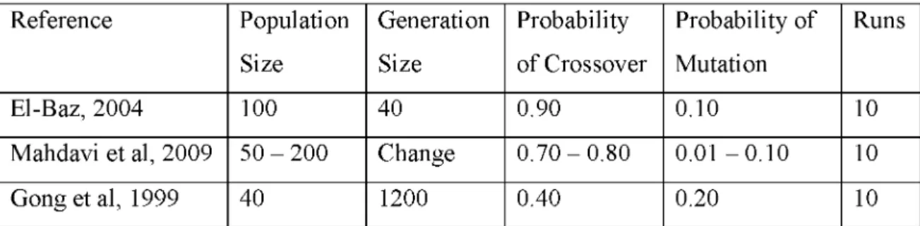
Table 2.2.1 GA- parameters used
Reference Population Size Generation Size Probability of Crossover Probability of Mutation Runs El-Baz, 2004 100 40 0.90 0.10 10
Mahdavi et al, 2009 50 - 200 Change 0.70 - 0.80 0.01 - 0.10 10
Gong et al, 1999 40 1200 0.40 0.20 10
In Table 2.2.1, the following observations can be made: the maximum size of population is
200, generation size is changeable and also the probability o f crossover is between 0.70
and 0.80 and the probability o f mutation is between 0.01 and 0.10.
Stop Rule: There are two points where the experiment can be stopped. One is when
maximum number o f generations is reached (El-Baz, 2004). The other is best value
becomes stable (Mantawy et al., 1999).
Two genetic algorithm codes written with different selection methods being used, the
selection methods used are SF and SS for producing new generation. SF is a fitness
function where best number o f solutions individual from all solutions is chosen where as
SS function is a survival function where calculating the total change by taking minimum
fitness value away from fitness o f each individual and summing up all. This way worst
A lgorithm GA
1. Population (pop) = create.random() 2. bs pop.Min().getCost() 3. W hile ( gs != G || bs != newbs) { 4. newbs bs 5. x = pop.selectbyRouletteWheel() 6. y = pop.selectbyRouletteWheel() 7. PM X (x,y) -> c, n 8. c = MutatebyInsert(c) n = MutatebyInsert(n) 9. pop = pop + (c , n)
10. 10.a newpop = SF (pop) Or 10.b. newpop = SS (pop) 11. pop.clear()
12. pop = newpop
13. bs pop.Min().getCost() 14. }
10.a SF { for (int k=0; k < P ; k++) { z = pop.Min().getFitness() } newpop.add(z) } 10.b SS { for (int k=0; k < P ; k++) { z = pop.selectbyRouletteWheel() } newpop.add(z) } Figure-2.2.1: Pseudocode GA
The variables in genetic algorithm implementations are: population (pop), new population
(newpop), individuals (x, y and z), children (c and n), old best solution (bs), new best
solution (newbs), number o f generation (gs), fitness function (SF), survival function (SS),
maximum number of generation (G), number of solution (P), probability of crossover
(CXP) and probability o f mutation (MP).
In Figure 2.2.1, until number o f solution (P) is reached, initial solutions are randomly
cost o f population (pop) and this solution is assigned to old best solution (bs) in line (2).
Until stopping rule (maximum number o f generations is reached or best solution becomes
stable) is met, the process continues in line (3-14). ‘b s’ is assigned to ‘newbs’ in line (4).
A solution (x) is selected by Roulette Wheel method in line (5). A solution (y) is selected
by Roulette Wheel method in line (6). Two children (c and n) are created by making PMX
crossover with x and y in line (7). These solutions (c and n) are mutated by Insert in line
(8) and ‘c’ and ‘n ’ are added to population (pop) in line (9). Two genetic algorithm codes
written with different selection methods being used, the selection methods used are SF
(line 10.a) and SS (line 10.b) for producing new generation. In line (10.a), until number of
solution (P) is reached, new generations are selected by using fitness function (SF). New
generations are added to ‘newpop’. In line (10.b), until number o f solution (P) is reached,
new generations are selected by using survival function (SS). New generations are added to
‘newpop’. In line (11), ‘pop’ is deleted. ‘newpop’ is assigned to ‘pop’ in line (12). One solution had the lowest cost o f population (pop) and this solution is assigned to old best
solution (bs) in line (13).
2.2.1. P aram eters T uned
There are some parameters as follows:
i. Selection (S) is set to either (1. genetic code : SF - fitness function or
2. genetic code : SS - survival function).
ii. Mutation probability (MP) is set to 0.05.
iii. Crossover probability (CXP) is set to 0.75.
iv. Maximum Generation (G) is set to either 40 or 400.
v. Number o f Solutions (P) is set to either 50,100 or 200.
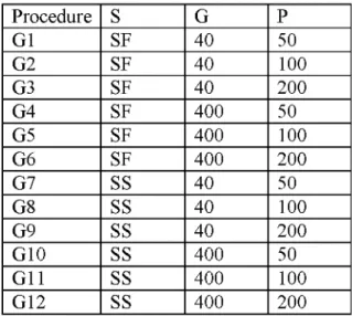
Depending on different combinations o f parameters 12 different genetic algorithm
Table 2.2.1.1 Parameter settings o f GA. Procedure S G P G1 SF 40 50 G2 SF 40 100 G3 SF 40 200 G4 SF 400 50 G5 SF 400 100 G6 SF 400 200 G7 SS 40 50 G8 SS 40 100 G9 SS 40 200 G10 SS 400 50 G11 SS 400 100 G12 SS 400 200
12 heuristic algorithms were tested on eight test problems. The results are given in (3.2).
2.3. S catter Search A lgorithm
Scatter search is an algorithm which does not allow same solutions and it is developed by
Glover in 1997. Due to duplicate solutions not being allowed in scatter search,
diversification should be considered very important. Applications o f scatter search
algorithms are investigated in Cung et al (1997).
Scatter search method starts with generating initial population. The fundamental idea is not
to allow duplicate solutions in Reference set (RefSet). Because o f this, diversification method is used in the population. Generation method is used to in the reference set where
Refset has b1 (better solution of population) and b2 (high diverse solution of population).
The reference set (RefSet) is developed by mutation operator. When there is no new
solution in RefSet, the experiment should be stopped.
Scatter search consists of six methods: diversification method, improvement method,
Generation method is used in the reference set where Refset has b1 (better solution) and
b2 (high diverse solution), reference set can be updated when a new solution which
satistifles the conditions as follows: new solution should have better cost function than the
solution with worst function in b1, also should be high divert to the reference set than the
solution with the worst divert in b2 which classifies b1 solutions as high quality and b2
solutions as high diversity (Marti et al., 2006).
High Diverse Solution: The more distance between two solutions, the solutions will have
the high diversity. The distance is defined as shown in Equation 2.3.1.
d(p,q) = En-1i=1 distance between pi+1 and pi in q (2.3.1)
Equation 2.3.1: Distance equation (Yuan et.al, 2007).
According to Equation 2.3.1, calculating distance between pi+1 and pi in q.
Diversification Method: As stated earlier diversification method is important since scatter
search does not allow duplications in the reference set, this is the reason why tabu list is
being used. The tabu list helps to reduce the computational effort to check duplication
solutions by every solution to be checked while they are in the tabu list, if the solution is
not a member of tabu list then it should be added to the list, if not the solution should be
discarded (Cung et al., 1997 ; Marti et al., 2006).
Improvement Method: Two improvement methods called Swap and Insert are used in this research; Swap and Insert mutation operator are defined as (2.1).
Selection Method: Roulette wheel selection and lexicographical order selection methods
are used in this research from selection methods. Roulette wheel selection is defined as in
(2.1). Lexicographical order selection is a simple sort method; the name o f the method
indicates the strings are compared in alphabetical order / numerical order, from left to right
Crossover Method: Two crossover methods are used PM X (Partially Matched Crossover)
and Combine method. PM X (Partially Matched Crossover) is defined in (2.1). Combine
Method is a crossover operator which produces new solutions from pairs o f reference
solutions where at least one new solution exists in the pair. The combine method has three
steps starting with choosing a start node then move left part o f the solutions “p1” and “p2”
to the right end position. Then, first node o f the parents is selected as combine solution “c” .
Second step is to compare the distance last selected node in “c” to the next node of “p1 ”
and “p2”, then short ones node should be chosen for the new rotation to “p1” and “p2” .
Third step which is repeating step 2 happens until combine solution “c” is finished (Yuan,
et al., 2007).
Reference Set Update M ethod is a method where Refset and new solutions are placed in
the tabu list, then b1 (better solution) and b2 (high diverse solution) are selected, then
Refset should be updated with b1 (better solution) and b2 (high diverse solution) (Marti et
al., 2006).
Stop Rule: The experiment should be stopped when there is no new solution in RefSet
(Marti et al., 2006).
Two scatter search algorithm codes provided in this research are (SPR and SLC), SPR
algorithm code uses roulette wheel selection method, pmx crossover method and insert
mutation method where as SLC consists of the following methods: lexicographical order
selection method, combine crossover method and swap mutation method. Scatter search
A lgorithm SS - SPR
1. Population (p) = create.random() 2. Diversification.method (p) 3. p =MutatebySwap(p) 4. CheckedbyTabuList (p)
5. RefSet = TabuList (b1) + TabuList (b2) 6. While (New Solution isn’t in the RefSet) 7. I 8. TabuList.clear() 9. x= SelectedByRouletteWheel() 10. y= SelectedByRouletteWheel() 11. PM X (x,y) ^ z, t 12. z = MutateByInsert (z) 13. t = M utateByInsert (t) 14. TabuList = RefSet
15. if (z.getCost() < t.getCost() && z 0 TabuList) 16. I TabuList = TabuList + z }
17. if (z.getCost() > t.getCost() && t 0 TabuList) 18. I TabuList = TabuList + t }
19. RefSet.update (b1 + b2) 20. }
Figure-2.3.1: Pseudocode SS (SPR)
The variables in scatter search SPR implementations are: population (p), individual
solutions (x and y), solutions (z and t), tabu list size (Tsize), number o f better solutions
(b1) and number o f high diverse solutions (b2).
In Figure 2.3.1, there is no solution in the tabu list. Until Tsize is reached, initial solutions
are randomly created and these solutions are assigned to ‘p ’ in line (1). Each solution is
checked by using diversification method that if a solution isn’t an element o f tabu list, a
solution adds to tabu list, otherwise discard this solution in line (2). Each solution is
mutated by Swap in line (3). Each solution is checked by using diversification method that
if a solution isn’t an element o f tabu list, it adds to tabu list, otherwise discard this solution
in line (4). Therefore, there are no duplicate solutions in tabu list. The reference set
(RefSet) has b1 (better solutions o f tabu list) and b2 (high diverse solutions o f tabu list) in
line (5). This process continues until there is no new solution in RefSet in line (6). Tabu
(9- 10) and solutions (z and t) are created by using PM X crossover with pairs (x and y) in
line (11). These solutions (z, t) are mutated by Insert in line (12 - 13). RefSet adds to
TabuList in line (14). If the fitness cost o f z is less than the fitness cost o f t and z isn’t an
element o f Tabu List, z will add to Tabu List in line (15 - 16). If the fitness cost o f z is
higher than the fitness cost o f t and t isn’t an element o f Tabu List, t will add to Tabu List
in line (17 - 18). Tabu List consists o f (z or t) and RefSet. Therefore, there is no duplicate
solution in Tabu List. RefSet is updated by consisting o f b1 (better solutions o f tabu list)
and b2 (high diverse solutions of tabu list) in line (19).
A lgorithm SS - SLC
1. Population (p) = create.random() 2. Diversification.method (p) 3. p =MutatebySwap(p) 4. CheckedbyTabuList (p)
5. RefSet = TabuList (b1) + TabuList (b2) 6. While (New Solution isn’t in the RefSet) 7. { 8. TabuList.clear() 9. x= SelectedByLexi cographicalorder() 10. y= S el ectedByLexicographicalorder() 11. Combine (x, y) -> z 12. z = MutatBySwap (z) 13. TabuList = RefSet 14. if (z 0 TabuList) { 15. TabuList = TabuList + z } 16. RefSet.update (b1 + b2) 17. } Figure-2.3.2: Pseudocode SS (SLC)
The variables in scatter search SLC implementations are: population (p), individual
solutions (x and y), solution (z), tabu list size (Tsize), number o f better solutions (b1) and
number o f high diverse solutions (b2).
In Figure 2.3.2, there is no solution in the tabu list. Until Tsize is reached, initial solutions
are randomly created and these solutions are assigned to ‘p ’ in line (1). Each solution is
solution adds to tabu list, otherwise discard this solution in line (2). Each solution is
mutated by Swap in line (3). Each solution is checked by using diversification method that
if a solution isn’t an element o f tabu list, it adds to tabu list, otherwise discard this solution
in line (4). Therefore, there are no duplicate solutions in tabu list. The reference set
(RefSet) has b1 (better solutions o f tabu list) and b2 (high diverse solutions o f tabu list) in
line (5). This process continues until there is no new solution in RefSet in line (6). Tabu
List is cleared in line (8). The pairs (x, y) are selected by lexicographical order in line (9
10) and solution (z) is created by using Combine crossover with pairs (x and y) in line (11).
This solution (z) is mutated by Insert in line (12). RefSet adds to TabuList in line (13). If z
isn’t an element o f Tabu List, z will add to Tabu List in line (15). Tabu List consists o f (z)
and RefSet. Therefore, there is no duplicate solution in Tabu List. RefSet is updated by
consisting of b1 (better solutions of tabu list) and b2 (high diverse solutions of tabu list) in line (16).
2.3.1. S catter Search A lgorithm - P aram eters
There are some parameters as follows:
i. Tabu List Size (Tsize) is set to either 30, 50 or 100. The tabu list is used to reduce
the computational effort of checking for duplicated solutions and also tabu list
doesn’t allow duplicate solutions. Therefore, Tsize is nearly bigger than sum o f b1
and b2 (Dai, 2008).
ii. Number o f high quality solutions (b1) is set to either 10 or 20. b1 has been taken
more than 20 (Dai, 2008).
iii. Number o f high diverse solutions (b2) is set to either 10 or 20. b2 has been taken
more than 20 (Dai, 2008).
iv. Mutation probability (MP) is set to 0.05.
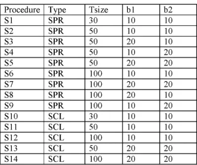
Depending on different combinations of parameters 14 different scatter search heuristics
are established. (Table 2.3.1).
Table 2.3.1 Parameter settings of SS
Procedure Type Tsize b1 b2
S1 SPR 30 10 10 S2 SPR 50 10 10 S3 SPR 50 20 10 S4 SPR 50 10 20 S5 SPR 50 20 20 S6 SPR 100 10 10 S7 SPR 100 20 20 S8 SPR 100 20 10 S9 SPR 100 10 20 S10 SCL 30 10 10 S11 SCL 50 10 10 S12 SCL 100 10 10 S13 SCL 50 20 20 S14 SCL 100 20 20
14 heuristic algorithms were tested on eight test problems. The results are given in (3.3).
2.4. G rasp A lgorithm
Greedy randomized adaptive search procedure (GRASP) is a method where at each step an
approximate solution is provided and best solution is generated from all solutions Grasp
starts with generating an initial population and initial solutions are created randomly until
the number of solutions is reached. The fundamental idea is to create restricted candidate
list (RCL) because of selecting the partial solutions which are developed by mutation
operators like Insert and Swap (Nehi and Gelareh, 2007). Grasp algorithm is shown in Figure-2.4.1.
Selection Method: roulette wheel selection method is used and defined in (2.1).
Improvement Method: swap and insert mutate operators are used and defined in (2.1). RCL
consists o f partial solutions (Nehi and Gelareh, 2007).
A lgorithm GX 1. Create_initial_population(pop) 2. oldv pop.getMin().getCost() 3. for ( i < maxi ) 4. { 5. Create_RCL ( 6. for(int i=0;i<population.size()/2;i++) 7. {s1 = selectByRouletteWheel(); 8. RCL.add(s1); 9. pop.remove(s1); } 10. ) 11. Update_Solution (
12. for(int k=0;k<RCL.size();k++) {uprs.add()}
13. upra = uprs;
14. uprm = uprs;
15. uprs.mutateBy Swap (mp); 16. uprm.mutateBylnsertion(mp);
17. if(uprs.getCost() < uprm.getCost() ) {gbest uprs
18. else gbest ^-uprm }
19. if (gbest < upra.getCost() ) { gbest gbest
20. else gbest upra, pop.add(upra) } 21. if (gbest == uprs.getCost() ) { pop.add (uprs) }
22. if (gbest == uprm.getCost()) { pop.add (uprm) } 23. return bestv pop.Min().getCost()
24. )
25. if (oldv < bestv) {bestv oldv, else bestv bestv } 26. }
Figure-2.4.1: Pseudocode GX
The variables in grasp implementations are: population (pop), solutions (s1, uprs, upra and uprm), restricted candidate list (RCL), iteration (i), maximum iteration (maxi), old best
solution (oldv), best solution (bestv), temp best solution (gbestv) and number of solution
(seed).
In Figure 2.4.1, initial solutions are created randomly and these solutions add to population
assigned to ‘oldv’ in line (2). Until the maximum iteration (maxi) is reached, the process
continues in line (3 - 26). RCL list is created in line (5- 10). Until population size is equal
to half (population/2), these solutions are selected by roulette wheel method in line (7) and
these solutions add to RCL list in line (8) and these solutions delete in the population (pop)
in line (9). Solutions are updated in line (11 - 24). Until RCL list size is reached, the
solutions o f RCL list add to ‘uprs’ in line (12). The solution (uprs) is assigned to ‘upra’ in
line (13). The solution (uprs) is assigned to ‘uprm ’ in line (14). The solution (uprs) is
mutated by Swap in line (15). The solution (uprm) is mutated by Insert in line (16). If
(uprs)’s cost is less than (uprm)’s cost, ‘uprs’ is assigned to ‘gbest’ , otherwise ‘uprm ’ is
assigned to ‘gbest’ in step (17 - 18). If ‘gbest’ is less than (upra)’s cost, return gbest,
otherwise ‘upra’ is assigned to ‘gbest’ and ‘upra’ adds to population (pop) in line (19 -
20). If ‘gbest’ is equal to uprs’s cost, ‘uprs’ adds to population (pop) in line (21). If ‘gbest’
is equal to uprm ’s cost, ‘uprm ’ adds to population (pop) in line (22). One solution which
has the lowest cost o f the population (pop), is set to ‘bestv’ in line (23). If ‘oldv’ is less than ‘bestv, return oldv else return bestv in line (25). When maximum iteration is reached,
the experiment should be stopped.
2.4.1. G rasp A lgorithm - P aram eters
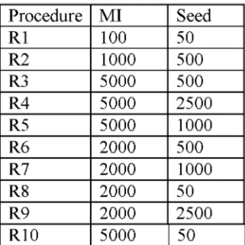
There are some parameters as follows:
i. Maximum iteration (MI) is set to 100, 1000, 2000 and 5000.
ii. Number o f solutions (seed) is set to 50, 500, 1000 and 2500.
iii. Mutation probability (MP) is set to 0.05.
Depending on different combinations of parameters 10 different grasp heuristics are
Table 2.4.1 Parameter settings o f GX Procedure MI Seed R1 100 50 R2 1000 500 R3 5000 500 R4 5000 2500 R5 5000 1000 R6 2000 500 R7 2000 1000 R8 2000 50 R9 2000 2500 R10 5000 50
3. EX PE R IM E N T A L RESU LTS
There are eleven problems defined in (Duman and Or, 2007)’s literature eight o f which we
have obtained. Due to this, only eight problems are tested in Laboratory o f Dogus
University.
Characteristics o f these tables are shown in Table 3.1.
Table 3.1: The number of components in each problem.
Problems # PS11AK08-9 146 PS11AK1011 159 PS11AK12-7 152 PS11AK15-4 170 PS11AK16-3 261 PS11AK16-4 262 PS11AK16-5 280 PS11AK17N3 185
Table 3.1 shows number o f components in departments.
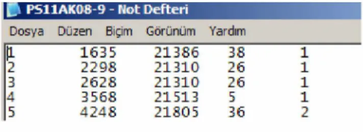
Table 3.2: The context o f test problem (PS11AK08-9).
PS11AK0S-9 - Not Defteri
Dosya Düzen Biçim Görünüm Yardım
|L 1635 21386 38 2 2298 21310 26 3 2628 21310 26 4 3566 21513 5
5 4248 2180 5 36
According to Table 3.2, PS11AK08-9 test has 5 different columns. First column contains
row number and increases by 1. Second is x-coordinate, third is y-coordinate, fourth is the
cell (department) where it is put and last is the type. It is the same for the rest o f the test
Detecting the best performing heuristic algorithm is complicated due to the fact that the
performance of a heuristic is dependent on the problem type which is determined by the
structure and relationship of problem parameters.
3.1. Sim ulated A nnealing - Test Results
12 heuristic procedures on eight test problems have been run ten times in order to get
detailed results. (See [Table 6.1] for a full tabulation in see Appendix). Out o f eight test
problems, the best average and the best solutions are displayed in (Table 3.1.1). Each test
problem is run for 10 times and there are total 120 ( 12 x 10) results for each test problem.
From 120 results the best solutions are indicated. (Table 3.1.1- Best solution) from each
procedure for each test case (10 times) the average solutions are calculated (Table 3.1.1 -
Average solution).
H8, H9, H15 and H 16’s results are worse than rest o f the results. Therefore, the
performance o f (Noi = N , R=20 and T=1000) parameters are better than the performance
o f (Noi = N 3/ 3, R=5 and T=100) parameters.
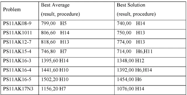
Table 3.1.1 SA - best average and best solution of problems
Problem Best Average (result, procedure) Best Solution (result, procedure) PS11AK08-9 799,00 H5 740,00 H14 PS11AK1011 806,60 H14 750,00 H13 PS11AK12-7 818,60 H13 774,00 H13 PS11AK15-4 746,80 H7 714,00 H6,H11 PS11AK16-3 1395,60 H14 1348,00 H12 PS11AK16-4 1441,60 H10 1392,00 H6,H14 PS11AK16-5 1502,20 H10 1454,00 H6 PS11AK17N3 1156,20 H7 1076,00 H14
Parameters of each procedure and successful results for testing are proposed in (Table
3.1.2). This table is supported by (Table 3.1.1). For instance out o f eight problems there is
only one best average and none o f the best solutions in H5 is in (Table 3.1.1). Looking at
H5, best average is 1 and best solution is 0 (Table 3.1.2). This value is used to compare the
performance of procedures.
We have come up with the idea that the highest number o f “best solution” is the best
heuristic procedure. This is the reason why time is not a concern on this research, each
procedure only works 10 times, and if run time is critical, the highest number o f “best
average” is the best heuristic procedure.
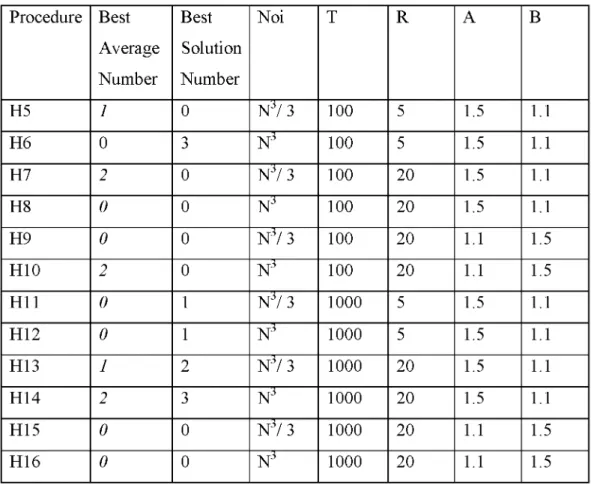
Table 3.1.2 SA - test results and parameters used
Procedure Best Average Number Best Solution Number Noi T R A B H5 1 0 N 3/ 3 100 5 1.5 1.1 H6 0 3 N 3 100 5 1.5 1.1 H7 2 0 N 3/ 3 100 20 1.5 1.1 H8 0 0 N 3 100 20 1.5 1.1 H9 0 0 N 3/ 3 100 20 1.1 1.5 H10 2 0 N 3 100 20 1.1 1.5 H11 0 1 N 3/ 3 1000 5 1.5 1.1 H12 0 1 N 3 1000 5 1.5 1.1 H13 1 2 N 3/ 3 1000 20 1.5 1.1 H14 2 3 N 3 1000 20 1.5 1.1 H15 0 0 N 3/ 3 1000 20 1.1 1.5 H16 0 0 N 3 1000 20 1.1 1.5
Looking at Table 3.1.2, H14 has 2 o f best average and 3 o f best solutions, whereas H14 is
and T=1000) parameters are the best. It is observed that using higher initial temperature
and higher number of iterations have positive effect on the performance o f the algorithm.
3 3
A numerical comparison shows that N iterations are better than N / 3 with respect to
heuristic procedures, which shows one percent benefit is observed more with H14 being
best heuristic procedure in Duman and Or (2007).
3.2. G enetic A lgorithm - Test Results
12 heuristic procedure on eight test problems have been run ten times in order to get the
results. (See [Table 6.2] for a full tabulation in see Appendix). Out o f eight test problems
the best average and the best solutions are listed in (Table 3.2.1). Each test problem is run for 10 times and there are total 120 ( 12 x 10) results for each test problem. From 120
results the best solutions are given in (Table 3.2.1- Best solution) from each procedure for each test case (10 times) the average solutions are calculated (Table 3.2.1 - Average
solution).
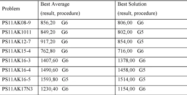
Between G1 and G12, G5 and G6 shows the best performance with parameters o f (S = SF,
G=400, P = 200) and also using SS (survival selection) G12 shows the best performance
between G7 and G12.
Table 3.2.1 GA- best average and best solution o f problems (G1-G12)
Problem Best Average (result, procedure) Best Solution (result, procedure) PS11AK08-9 856,20 G6 806,00 G6 PS11AK1011 849,20 G6 802,00 G5 PS11AK12-7 917,20 G6 854,00 G5 PS11AK15-4 762,80 G6 716,00 G6 PS11AK16-3 1407,60 G6 1378,00 G6 PS11AK16-4 1490,60 G6 1458,00 G5 PS11AK16-5 1593,80 G5 1514,00 G5 PS11AK17N3 1230,40 G6 1154,00 G6
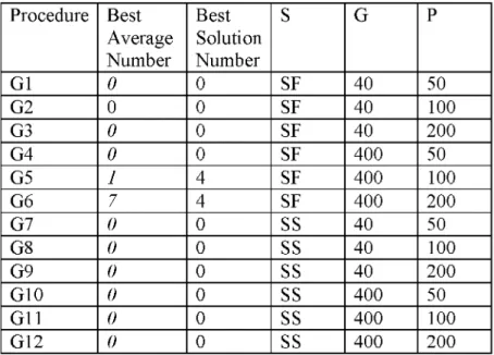
Parameters of each procedure and successful results for testing are proposed in (Table
3.2.2). This table is supported by (Table 3.2.1). For instance out o f eight problems there is
only one best average and four o f the best solutions in G5 is in (Table 3.2.1). Looking at
G5, best average is 1 and best solution is 4 (Table 3.2.1). This value is used to compare the
performance of procedures.
Table 3.2.2 GA- test results and parameters used
Procedure Best Average Number Best Solution Number S G P G1 0 0 SF 40 50 G2 0 0 SF 40 100 G3 0 0 SF 40 200 G4 0 0 SF 400 50 G5 1 4 SF 400 100 G6 7 4 SF 400 200 G7 0 0 SS 40 50 G8 0 0 SS 40 100 G9 0 0 SS 40 200 G10 0 0 SS 400 50 G11 0 0 SS 400 100 G12 0 0 SS 400 200
G6 is the best heuristic procedure with 7 o f best average and 4 o f best solutions between
G1 and G12. Per the results the performance o f (S = SF, G = 400 and P = 200) parameters
are best. It is observed that selection method (SF), higher initial population and higher
number o f generations have positive effect on the performance o f the algorithm. New
generations are created by fitness selection method SF where best number o f solutions
among all solutions is chosen without taking worst number o f solutions into account.
Otherwise, parameters o f G12 (S= SS, G = 400 and P = 200) which has a better performance between G7 and G12. It is observed using higher initial population and higher
number o f generations has positive affect on the performance o f the algorithm. New
generations are created using SS (Survival selection) which allows worst solutions to be chosen. As a result fitness selection is better than survival selection.
3.3. S catter Search - Test Results
14 heuristic procedure on eight test problems have been run ten times in order to get the
results. (See [Table 6.3] for a full tabulation in see Appendix). Out o f eight test problems
the best average and the best solutions are listed in (Table 3.3.1). Each test problem is run
for 10 times and there are total 140 (14 x 10) results for each test problem. From 140
results the best solutions are given in (Table 3.3.1- Best solution) from each procedure for
each test case (10 times) the average solutions are calculated (Table 3.3.1 - Average
solution).
S3, S5 and S7 show the best performance between S1 and S14. SPR shows better
performance than SLC.
Table 3.3.1 SS - best average and best solution o f problems (S1 - S14)
Problem Best Average (result, procedure) Best Solution (result, procedure) PS11AK08-9 993,2 S5 870,0 S5 PS11AK1011 976,6 S5 858,0 S5 PS11AK12-7 1028,8 S5 886,0 S5 PS11AK15-4 835,8 S5 772,0 S5 PS11AK16-3 1614,6 S5 1284,0 S3 PS11AK16-4 1599,2 S7 1450,0 S7 PS11AK16-5 1802,6 S5 1540,0 S5 PS11AK17N3 1494,0 S5 1248,0 S5
Parameters of each procedure and successful results for testing are proposed in (Table
3.3.2). This table is supported by (Table 3.3.1).
Procedure Best Average Number Best Solution Number Tsize B1 B2 S1 0 0 30 10 10 S2 0 0 50 10 10 S3 0 1 50 20 10 S4 0 0 50 10 20 S5 7 6 50 20 20 S6 0 0 100 10 10 S7 1 1 100 20 20 S8 0 0 100 20 10 S9 0 0 100 10 20 S10 0 0 30 10 10 S11 0 0 50 10 10 S12 0 0 100 10 10 S13 0 0 50 20 20 S14 0 0 100 20 20
S5 is the best heuristic procedure with 7 o f best average and 6 o f best solutions. As per the
results the performance o f (Tsize = 50, b1 = 20 and b2 = 20) parameters are the best.
b2 will have an opportunity to choose worst solution when Tsize has a very high value
(Tsize is bigger than sum o f b1 and b2). The performance o f SPR (S1 - S9) which uses
roulette wheel selection method, pmx crossover method and insert mutation method, is
better than SCL (S10 - S14) using leoxical order selection method, combine crossover
method and swap mutation. According to SPR, roulette wheel selection method allows for
worst solution (b) to perform PM X crossover therefore two solutions (a, c) are occurred
and two solutions (a, c) are mutated by insert and solution which has the lowest cost o f the
three solutions (a, b or c) is added to population. Furthermore, number o f worst solutions is
less comparing to iterations. According to SCL, leoxicalorder selection chooses a solution
orderly. One solution is produced by combined crossover o f solutions. A solution is
mutated by swap, and then a solution adds to population, where number o f best solutions
will be less than number o f best solutions before iterations.
10 heuristic procedure on eight test problems have been run ten times in order to get the
results. (See [Table 6.4] for a full tabulation in see Appendix). Out o f eight test problems
the best average and the best solutions are listed in (Table 3.4.1). Each test problem is run for 10 times and there are total 100 (10 x 10) results for each test problem. From 100
results the best solutions are given in (Table 3.4.1- Best solution) from each procedure for each test case (10 times) the average solutions are calculated (Table 3.4.1 - Average
solution).
Table 3.4.1 GX - best average and best solution o f problems (R1-R10)
Problem Best Average (result, procedure) Best Solution (result, procedure) PS11AK08-9 939,0 R10 852 R10 PS11AK1011 936,6 R3 836 R10 PS11AK12-7 982,2 R4 884 R3 PS11AK15-4 804,8 R5 742 R4 PS11AK16-3 1527,8 R4 1444 R3 PS11AK16-4 1571,8 R5 1486 R5 PS11AK16-5 1687,2 R4 1556 R5 PS11AK17N3 1398,4 R3 1314 R3
Parameters of each procedure and successful results for testing are proposed in (Table
3.4.2). This table is supported by (Table 3.4.1).
Procedure Best Average Number Best Solution Number MI Seed R1 0 0 100 50 R2 0 0 1000 500 R3 2 3 5000 500 R4 3 1 5000 2500 R5 2 2 5000 1000 R6 0 0 2000 500 R7 0 0 2000 1000 R8 0 0 2000 50 R9 0 0 2000 2500 R10 1 2 5000 50
R4 is the best heuristic procedure with 3 o f average and 1 of best solution. The results
show that the performance o f (MI = 5000, Seed = 2500) parameters are the best.Using higher maximum iteration and higher number o f solutions help performance o f algorithm
to increase.
CM (Comparison o f Methods) developed using Java is used to compare performance of
Simulated Annealing, Genetic Algorithm, Scatter Search and Grasp algorithms. (Duman
and Or, 2007)’s literature problems are tested using CM with each metaheuristic
algorithms.
There are two comparisons side to tests, one is best procedure o f methods and the other is
comparing best solution and best average o f each problem. In Part 3 comparisons o f these
algorithms are provided.
Comparison o f M ethod’s Best Procedure:
H14 is the best procedure o f Simulated annealing. G6 is the best procedure o f Genetic
algorithm. S5 is the best procedure o f Scatter search. R4 is the best procedure o f Grasp.
Table 4.1.1 Best average o f algorithms
Problem Best Average Best
Average H14 G6 S5 R4 PS11AK08-9 820 856,2 993,2 967,4 H14 PS11AK1011 806,6 849,2 976,6 939,4 H14 PS11AK12-7 842,2 917,2 1028,8 982,8 H14 PS11AK15-4 752 762,8 835,8 806,6 H14 PS11AK16-3 1395,6 1407,6 1614,6 1527,8 H14 PS11AK16-4 1461,2 1490,6 1684,2 1582,2 H14 PS11AK16-5 1542,6 1603,8 1802,2 1687,2 H14 PS11AK17N3 1165,4 1230,4 1494,0 1402,8 H14
The following observations are made from Table 4.1.1, H14 is the best average o f all these
problems. Simulated Annealing has best average for QAP test problems. According to that
results, the performance o f (Noi = N , R=20, a=1.5, b=1.1 and T=1000) parameters are
best. Orderly, the performances o f others are G6, R4 and S5. Table 4.1.2 Best solution o f algorithms
Problem Best Solution Best Solution H14 G6 S5 R4 PS11AK08-9 740 806 870 904 H14 PS11AK1011 756 808 858 872 H14 PS11AK12-7 800 858 886 928 H14 PS11AK15-4 718 716 772 742 G6 PS11AK16-3 1370 1378 1398 1450 H14 PS11AK16-4 1392 1458 1502 1510 H14 PS11AK16-5 1474 1546 1540 1632 H14 PS11AK17N3 1076 1154 1248 1320 H14
Looking at Table 4.1.2, H14 is the best solution o f 7 problems, but G6 is the best solutions o f the PS11AK15-4 problems. Simulated Annealing has best solution for solving QAP test
problems. Orderly, the performances o f others are G6, S5 and R4.
Comparison o f Each Problem ’s Best Solution and Best Average:
H5, H7, H10, H13 and H14 are the best average o f each problem in Simulated Annealing.
G6 and G5 are the best average of each problem in Genetic Algorithm. S5 and S7 are the
best average o f each problem in Scatter Search. R3, R4, R5 and R10 are the best average of
each problem in Grasp.
Table 4.2.1: Best average o f each problem in algorithms
Problem Best Average Best
Average SA GA SS GX PS11AK08-9 799 H5 856,2 G6 993,2 S5 939,0 R10 H5 PS11AK1011 806,6 H14 849,2 G6 976,6 S5 936,6 R3 H14 PS11AK12-7 818,6 H13 917,2 G6 1028,8 S5 982,8 R4 H13 PS11AK15-4 746,8 H7 762,8 G6 835,8 S5 804,8 R5 H7 PS11AK16-3 1395,6 H14 1407,6 G6 1614,6 S5 1527,8 R4 H14 PS11AK16-4 1441,6 H10 1490,6 G6 1599,2 S7 1571,8 R5 H10 PS11AK16-5 1502,2 H10 1593,8 G5 1802,6 S5 1687,2 R4 H10 PS11AK17N3 1156,2 H7 1230,4 G6 1494 S5 1398,4 R3 H7
Table 4.2.1 results are as: H5, H7, H10, H13 and H14 are the best average in each
problem. Simulated Annealing has best average o f all eight problems. Orderly, the
performances o f others are Genetic algorithm, Grasp and Scatter search.
H6, H11, H12, H13 and H14 are the best solutions o f each problem in Simulated
Annealing. G6 and G5 are the best solutions o f each problem in Genetic Algorithm. S3, S5
and S7 are the best solutions o f each problem in Scatter Search. R3, R4, R5 and R10 are
the best solutions o f each problem in Grasp.
Table 4.2.2: Best solution o f each problem in SA, GA, SS, GX
Problem Best Solution Best
Solution SA GA SS GX PS11AK08-9 740 H14 806 G6 870 S5 852 R10 H14 PS11AK1011 750 H13 802 G5 858 S5 836 R10 H13 PS11AK12-7 774 H13 854 G5 886 S5 884 R3 H13 PS11AK15-4 714 H6, H11 7 1 6 G6 772 S5 742 R4 H6,H11 PS11AK16-3 1348 H12 1378 G6 1284 S3 1444 R3 S3 PS11AK16-4 1392 H6,H14 1458 G5 1450 S7 1486 R5 H6,H14 PS11AK16-5 1454 H6 1514 G5 1540 S5 1556 R5 H6 PS11AK17N3 1076H14 1154 G6 1248 S5 1314 R3 H14
According to Table 4.2.2, the best solutions are H6, H11, H13, H14 and S3. Simulated
Annealing has best solutions o f 7 problems, but a PS11AK16-3 problem is S3 as Scatter
search.
4.1. Sum m ary
In this study a program called CM is developed to compare performance o f metaheuristic
algorithms in Eclipse platform. Algorithms compared are simulated annealing, genetic
algorithm, scatter search and grasp. (Duman and Or, 2007)’s literature problems are solved
using these algorithms and compared by CM. As stated before, deciding the best
performing heuristic is complicated by the fact that the performance o f a heuristic depends
on the context o f the problem, which is determined the structure and relationships of