Selçuk J. Appl. Math. Selçuk Journal of Vol. 13. No. 2. pp. 69-78, 2012 Applied Mathematics
On the Extremes of Surplus Process in Compound Binomial Model Serkan Eryilmaz1, Altan Tuncel2, Fatih Tank3
1Atilim University, Department of Industrial Engineering 06836, Incek, Ankara Turkiye 2K¬r¬kkale University, Faculty of Science and Arts, Department of Statistics Yahsihan,
Kirikkale, Turkiye
3Ankara University, Faculty of Science, Department of Statistics, 06100 Tandogan,
Ankara, Turkiye e-mail:tank@ ankara.edu.tr
Received Date: November 28, 2012 Accepted Date: December 1, 2012
Abstract. In this paper we study the minimum and maximum levels of surplus process in compound binomial model. These extremes are potentially useful for an investment strategy and …nancial arrangements of an insurance company. We obtain recursive equations for the marginal as well as joint distributions of the minimum and maximum values of the surplus process occurred up to period n under the condition that the insurance company survives at time n. We present illustrative computational results for geometric claim size distribution.
Key words: Compound binomial model; Recurrence formula; Surplus process. 2000 Mathematics Subject Classi…cation: 60H30, 91B30, 62P05.
1. Introduction
One of the most important stochastic process for an insurance company is called a surplus process which can be de…ned as discrete or continuous time in actuarial risk theory. Estimation of the surplus at a certain time is essential for the insurance companies due to their future investment strategies and actions to be taken just before ruin. In this regard, maximum and minimum level of the surplus and its related quantities should be controlled by the companies. An insurer’s surplus might be modeled as the result of two quantities: a premium income collected continuously at the rate of c, and an outgoing sequence of
insurance claims. In discrete time model, insurer’s surplus process, which is called Sparre Anderson Risk Model, up to time t can be de…ned by
(1) Ut= u + ct
t X j=1
Yj
with U0= u; where u is the amount of initial reserve, the premium income is c per each period, and Yjis the eventual claim amount in period j. For simplicity, throughout the paper we assume that c = 1.
Let Ij be a binary random variable representing the claim occurrence. That is Ij = 1 if a claim occurs in period j and Ij= 0, otherwise. For j 1; de…ne Yj = IjXj; where the random variable Ij and the individual claim amount random variable Xj are independent in each time period. The random variable Xj is strictly positive and fXj; j 1g forms a sequence of iid random variables with probability mass function (p.m.f.) f (x) = P fX = xg : Under this assumptions, the process (1) can be rewritten as
(2) Ut= u + t
Nt
X j=1
Xj;
where u is non negative integer, Nn is the number of claims up to time n and Xj is the amount of jth claim. It is assumed that Xj random variables are independent and identically distributed (i.i.d.) and independent of the claim number process. Ruin of insurer’s occurs when Ut 0 for some t 1. Thus, the random time to ruin is de…ned as
T = inf ft > 0 : Ut 0g :
Let the random indicators I1; I2; ::: be independent with p = P fIj= 1g ; then the model (1) is called the compound binomial model and
P fNn = kg = Cnkpk(1 p)n k; k = 0; 1; :::; n:
The compound binomial model has been …rst proposed by Gerber (1988 a,b). Distributional properties of some actuarial quantities associated with compound binomial model have been studied in Shiu (1989), Michel (1989), Willmot (1993), Dickson (1994) and De Vylder and Marceau (1996). The compound binomial model, as a discrete time version of the classical compound Poisson model of risk theory has been widely studied in a recent literature (see, e.g. Yuen and Guo (2006), Liu and Zhao (2007), Hu and Zhimin (2010), Bao and Wang (2010), Ming et al. (2010), Eryilmaz (2012)). The model has been named as compound Markov binomial model whenever I1; I2; ::: is a Markov process. The latter case has been studied by Cossette et al. (2003), Cossette et al. (2004), Yuen and Guo (2006) and Liu and Zhao (2007).
The minimum and maximum levels of certain risk related stochastic processes have always become important for various purposes. In this paper we study
extreme levels of the surplus process (1) occurred up to period n under the condition that the insurance company survives at time n. Let Mn and Kn denote respectively the maximum and minimum levels of the surplus process up to period n, where P fT > ng > 0, i.e.
Mn= max
1 t nUt , Kn = min1 t nUt:
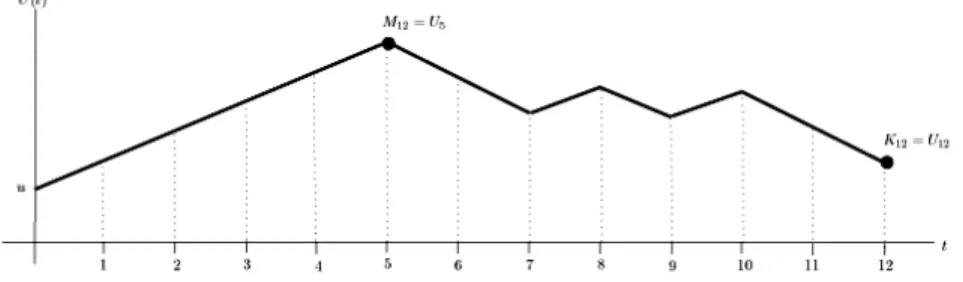
These random quantities might be useful for understanding the behavior of a certain portfolio over the periods. Although the ruin occurs when the value of the surplus process falls below zero, a positive threshold for the values of the surplus process might be a barrier for particular strategies of an insurance company. More explicitly, the company may want to know that the surplus never falls below a …xed positive threshold k up to a …xed period while it survives. In such a case, we need to evaluate the probability PufKn k j T > ng :A simple graphical representation of Mn and Kn processes is given in Figure 1.
Figure 1. A simple realization of the processes
The remainder of the present paper is organized as follows: Section 2 presents recursive equations to compute marginal and joint distributions of Mn and Kn under the condition T > n. Section 3 gives means and variances of Mn and Kn and the covariance between them for zero-truncated geometric claim size distribution.
2. Distributions of Extremes For u = 1; 2; ::: and n 0, de…ne
(u; n) = PufT > ng ; (u; n; k) = PufMn k; T > ng ; (u; n; k) = PufKn k; T > ng ; (u; n; k; l) = PufMn k; Kn l; T > ng :
The following recursive equation for the survival function of T can be obtained by conditioning on the time and the amount of the …rst claim.
(3) (u; n) = 8 > < > : 1 if n = 0 n X t=1 pqt 1 u+t 1X x=1 f (x) (u + t x; n t) + (1 p)n if n > 0. Theorem 1. For u = 1; 2; ::: PufMn k j T > ng = (u; n; k) (u; n) ; where
(a)If k u + n and n 0; (u; n; k) = (u; n); (b)If u k < u + n and n 0; (4) (u; n; k) = kXu+1 t=1 pqt 1 u+t 1X x=max(1;u+t k) f (x) (u + t x; n t; k):
Proof. The proof is immediate for k u+n since in this case Pu n
Mn(1) k o
= 1. For u k < u + n; let W1denote the waiting time for the …rst claim. Then,
(5) PufMn k; T > ng = 1 X t=1 PufU1 k; :::; Un k; T > n j W1= tg pqt 1 If t n then P fU1= u + 1; :::; Ut 1= u + t 1g = 1 and PufU1 k; :::; Un k; T > n j W1= tg = PufUt k; Ut+1 k; :::; Un k; T > n t j W1= tg ;
for t k u + 1. Noting that Ut> 0 for t n since the ruin occurs after period n and then by conditioning on the value of the …rst individual claim one obtains
PufUt k; Ut+1 k; :::; Un k; T > n t j W1= tg
(6) =
u+t 1X x=max(1;u+t k)
f (x)Pu+t xfMn t k; T > n tg ;
for t k u + 1. For t > n, P fMn= u + ng = 1. Thus PufMn k; T > ng = 0;
if k < u + n and t > n. Thus using (6) in (5) one obtains PufMn k; T > ng = = kXu+1 t=1 pqt 1 u+t 1X x=max(1;u+t k) f (x)Pu+t xfMn t k; T > n tg
for u k < u + n and hence the proof is complete. Theorem 2. For u = 1; 2; :::
PufKn k j T > ng =
(u; n; k) (u; n) ; where
(a)If k u and n = 0; (u; n; k) = 1; (b)If k u + 1 and n > 0; (u; n; k) = n X t=max(1;k u+1) pqt 1 u+t kX x=1 f (x) (u + t x; n t; k) + (1 p)n:
Proof. The proof is obvious for k u and n = 0. For k u+1, by conditioning on the …rst claim occurrence time,
PufKn k; T > ng (7) = 1 X t=1 PufU1 k; :::; Un k; T > n j W1= tg pqt 1:
If t n and k u + 1 we have PufU1 k; :::; Ut 1 k j W1= tg = 1, and PufU1 k; :::; Un k; T > n j W1= tg
= PufUt k; :::; Un k; T > n t j W1= tg and if t > n and k u + 1;
(8) PufU1 k; :::; Un k j W1= tg = 1:
For t n and k u + 1; by conditioning on the value of the …rst individual claim one obtains
PufUt k; :::; Un k; T > n t j W1= tg
(9) =
u+t kX x=1
Using (8) and (9) in (7), PufKn k; T > ng = n X t=max(1;k u+1) pqt 1 u+t kX x=1 f (x)Pu+t xfKn t k; T > n tg + 1 X t=n+1 pqt 1
which completes the proof of part (b).
Theorem 3. For u = 1; 2; ::: , the joint cdf of Mn and Kn is given by (10) PufMn k; Kn l j T > ng = (u; n; k) (u; n) (u; n; k; l + 1) (u; n) ; where
(a)If n = 0 and u l; (u; n; k; l) = (u; n; k); (b)If n 0 and k u + n, (u; n; k; l) = (u; n; l); (c)If u k < u + n; u + 1 l; k > l and n > 0; (u; n; k; l) = kXu+1 t=max(1;l u+1) pqt 1 u+t lX x=max(1;u+t k) f (x) (u + t x; n t; k; l):
Proof. The …rst and second parts readily follow since
PufMn k; Kn l; T > ng = PufMn k; T > ng ; for n = 0 and u l; and
PufMn k; Kn l; T > ng = PufKn l; T > ng ;
for n 0 and k u + n: Part (c) can be proved similar to the proofs of Theorem 1 and Theorem 2 because
(u; n; k; l) = PufMn k; Kn l; T > ng
=X
t 1
Pufl U1 k; :::; l Un k; T > n j W1= tg pqt 1: Equation (10) follows from
PufMn k; Kn l j T > ng
= PufMn k j T > ng PufMn k; Kn l + 1 j T > ng : 3. Numerical Results
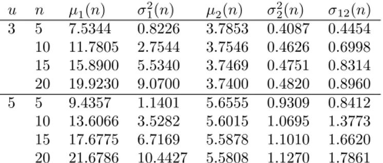
In this section we compute means and variances of Mn and Kn and the co-variance between them for the case when the individual claim size distribu-tion is zero-truncated geometric distribudistribu-tion with pmf f (x) = (1 ) x 1; x = 1; 2; ::: . In Tables 1 and 2, we compute 1(n) = E(Mn j T > n); 21(n) = V ar(Mn j T > n); 2(n) = E(Kn j T > n); 22(n) = V ar(Kn j T > n) and
u n 1(n) 2 1(n) 2(n) 22(n) 12(n) 3 5 7.5344 0.8226 3.7853 0.4087 0.4454 10 11.7805 2.7544 3.7546 0.4626 0.6998 15 15.8900 5.5340 3.7469 0.4751 0.8314 20 19.9230 9.0700 3.7400 0.4820 0.8960 5 5 9.4357 1.1401 5.6555 0.9309 0.8412 10 13.6066 3.5282 5.6015 1.0695 1.3773 15 17.6775 6.7169 5.5878 1.1010 1.6620 20 21.6786 10.4427 5.5808 1.1270 1.7861
Table 1. Means, variances and covariances of Mn and Kn when p = 0:07: u n 1(n) 21(n) 2(n) 22(n) 12(n) 3 5 7.3480 1.0809 3.6978 0.5523 0.6033 10 11.3126 3.4831 3.6539 0.6232 0.9247 15 15.0789 6.9852 3.6423 0.6408 1.1043 20 18.7458 11.2664 3.6381 0.6471 1.1874 5 5 9.2114 1.4850 5.5141 1.2602 1.1262 10 13.0684 4.4691 5.4341 1.4499 1.8281 15 16.7742 8.3674 5.4075 1.5176 2.2148 20 20.4099 13.0277 5.3987 1.5426 2.4156
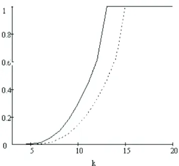
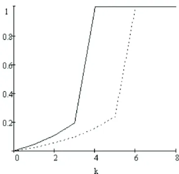
Table 2. Means, variances and covariances of Mn and Kn when p = 0:1: In Figures 2 and 3, we sketch the graphs of cumulative distribution functions of Mn and Kn for p = 0:1 and n = 10:
The results in Tables 1-2 and Figures 2-3 allow us to present the following conjectures: p1 p2 =) n Mn(1)j T1> n o u st n Mn(2)j T2> n o u; n1 n2 =) fMn1 j T > n1gu stfMn2 j T > n2gu; u1 u2 =) n Mn(1)j T1> n o u1 st n Mn(2)j T2> n o u2 ; p1 p2 =) n Kn(1)j T1> n o u st n Kn(2)j T2> n o u; n1 n2 =) fKn1 j T > n1gu stfKn2 j T > n2gu; u1 u2 =) n Kn(1)j T1> n o u1 st n Kn(2)j T2> n o u2 :
Figure 2. Cumulative distribution function of Mn given T > n: The solid line is for u = 3 and the dashed line is for u = 5
Figure 3. Cumulative distribution function of Kn given T > n. The solid line is for u = 3 and the dashed line is for u = 5.
References
1. Bao, Z., Wang, J. (2010), On the discountedpenaltyfunction in the discrete time stationary renewa lrisk model, Journal of Computational and Applied Mathematics, 234(3),557-562.
2. Cossette, H., Landriault, D., Marceau, É. (2003). Ruin probabilities in the com-pound Markov binomial model. Scandinavian Actuarial Journal, 4, 301-323.
3. Cossette, H., Landriault, D., Marceau, É. (2004). Exact expressions and upper bound for ruin probabilities in the compound Markov binomial model. Insurance: Mathematics and Economics, 34, 449-466.
4. De Vylder, F., Marceau, E. (1996). Classical numerical ruin probabilities. Scandi-navian Actuarial Journal, 109-123.
5. Dickson, D.C.M. (1994) Some comments on the compound binomial model. ASTIN Bulletin, 24, 33-45.
6. Eryilmaz, S. (2012) On distributions of runs in the compound binomial risk model, Methodology and Computing in Applied Probability, DOI: 10.1007/s11009-012-9303-x 7. Gerber, H. (1988). Mathematical fun with the compound binomial process. ASTIN Bulletin 18, 161-168.
8. Gerber, H. (1988b). Mathematical fun with ruin theory. Insurance: Mathematics and Economics, 7, 15-23.
9. Hu, Y., Zhimin, Z., (2010), On adiscreteriskmodel with two-sided jumps, Journal of Computational and Applied Mathematics, 234(3),835-844.
10. Liu, G., Zhao, J. (2007). Joint distributions of some actuarial random vectors in the compound binomial model. Insurance: Mathematics and Economics, 40, 95-103. 11. Michel, R. (1989). Representation of a time-discrete probability of eventual ruin. Insurance: Mathematics and Economics, 8, 149-152.
12. Ming, R. , He, X., Hu, Y.., Liu., J. (2010) Uniform estimate on …nite time ruin probabilities with random interest rate. Acta Mathematica Scientia, 30, 688-700. 13. Rotar, V.I. (2006). Actuarial models: the mathematics of insurance, Chapman & Hall/CRC.
14. Shiu, E., (1989). The probability of eventual ruin in the compound binomial model. ASTIN Bulletin, 19, 179-190.
15. Willmot, G.E. (1993). Ruin probabilities in the compound binomial model. In-surance: Mathematics and Economics, 12, 133-142.
16. Yuen, K-C., Guo, J. (2006). Some results on the compound Markov binomial model. Scandinavian Actuarial Journal, 3, 129-140.