M a p Building from Range D a t a Using
Mathematical Morphology
Billur Barshan and Deniz Ba§kent
7.1 Introduction
This chapter presents a novel method for surface profile extraction using multiple sensors. The approach presented is based on morphological pro-cessing techniques to fuse the range data from multiple sensor returns in a manner that directly reveals the surface profile. The method has the in-trinsic ability of suppressing spurious readings due to noise, crosstalk, and higher-order reflections, as well as processing multiple reflections informa-tively. The approach taken is extremely flexible and robust, in addition to being simple and straightforward. It can deal with arbitrary numbers and configurations of sensors as well as synthetic arrays. The algorithm is ver-ified both by simulations and experiments in the laboratory by processing real sonar data obtained from a mobile robot. The results are compared to those obtained from a more accurate structured-light system, which is however more complex and expensive.
Perception of its surroundings is a distinguishing feature of an intelli-gent mobile robot. An inexpensive, yet efficient and reliable approach to perception is to employ multiple simple sensors coupled with appropriate data processing.
Sonar sensors are robust and inexpensive devices, capable of providing accurate range data, and have been widely used in robotics applications. However, as we have seen already in this book, the angular resolution of sonar sensors is low, resulting in an uncertainty in the location of the object encountered. Furthermore, data from these sensors are often considered difficult to interpret due to specular reflections from most objects, especially when multiple or higher-order reflections are involved.
In robotics, most of the research on sonar has focused on surfaces with fixed or piecewise-constant curvature, mostly composed of target
primi-111 Copyright © 2001. World Scientific. All rights reserved. May not be reproduced in any form without permission from the publisher, except fair uses permitted under U.S. or applicable copyright law.
tives such as planes, corners, edges, and cylinders [Ayrulu and Barshan 98; Barshan and Kuc 90; Hong and Kleeman 97; Kleeman and Kuc 95; Kuc and Siegel 87; Leonard and Durrant-Whyte 91; Peremans 93]. In an earlier study which considers surfaces with varying curvature, a purely an-alytical approach is taken using ultrasonic echo trajectories and differential geometry to extract the surface features [Brown 86].
Sonar sensors have also been extensively used for map building and ob-stacle avoidance in robotics. The different geometric approaches in map building basically fall into two primary categories: feature-based and
grid-based. Feature-based approaches are based on extracting the geometry
of the environment from sensor data as the first step in data interpreta-tion (e.g. edge detecinterpreta-tion, straight-line or curve fitting to obstacle bound-aries) [Cox 91; Crowley 85; Crowley 89; Drumheller 97; Grimson and Lorano-Perez 84]. Many researchers have reported the extraction of line segments from sonar data as being difficult and brittle and have proposed alternative feature-based approaches [Kuc and Siegel 87; Leonard and Durrant-Whyte 91; Leonard et al 92]. Approaches based on physical model-based reason-ing, including classification of environmental features into target primitives discussed earlier [Ayrulu and Barshan 98; Barshan and Kuc 90; Bozma 92; Hong and Kleeman 97; Kleeman and Kuc 95] can also be considered feature-based methods.
An alternative representation is the certainty or occupancy grid (see chapter 4 section 4.1.1.1). Although grid-based methods have their limi-tations in terms of memory and resolution, they are advantageous in that they do not commit to making difficult geometric decisions early in the data interpretation process. On the other hand, since different target types are not explicitly represented, it is not as easy to predict what sonar data will be observed from a given position and to give account of individual sonar readings. Typically, when sufficient sensor data have been collected in the grid cells, the data are matched or correlated with a global model. This process can be computationally intensive and time consuming depending on the cell resolution of the grid.
In [Wallner and Dillman 95], a hybrid method is presented for updating the local model of the perceivable environment of a mobile robot. Unlike earlier grid-based approaches, local grids can be used in dynamic environ-ments. The method combines the advantages of feature- and grid-based environment modeling techniques. More detail on the different approaches
to map building can be found in [Borenstein et al 96].
The approaches described above are often limited to elementary target types or simple sensor configurations. On the other hand, the method pre-sented in this chapter is aimed at the determination of arbitrary surface profiles which are typically encountered in mines, rough terrain, or under-water. The approach is completely novel in that morphological processing techniques are applied to sonar data to reconstruct the profile of an
arbitrar-ily curved surface. It can also be looked at as a novel method for solving a
class of nonlinear reconstruction (inverse) problems. It is important to un-derline that morphological processing is employed here to process the sonar map of the surface being constructed in the robot's memory. The method has sufficient generality to find application in other ranging systems such as radar, optical sensing and metrology, remote sensing, and geophysical exploration.
Prom a map-building perspective, this method can also be considered as a hybrid of feature- and grid-based methods: Initially, the environment is discretised into rectangular grids. After accumulation of sufficient amount of data, a curve-fitting procedure is employed to extract the geometry of the surface under investigation. The present approach is advantageous over probability-based grid methods since it allows the use of a much finer phys-ical grid. This is because the approach does not rely on accumulation of multiple measurements in each cell. From a different perspective, although it is possible to interpret this method as a spatial voting scheme where cells are locally supported by their neighbours, we find it more appropri-ate to look at it from a nonlinear signal reconstruction perspective where morphological processing is used to extract reinforced features in the arc map.
The method is extremely flexible in that it can equally easily handle ar-bitrary sensor configurations and orientations as well as synthetic arrays ob-tained by moving a small number of sensors. As already mentioned above, a commonly noted disadvantage of sonar sensors is the difficulty associated with handling spurious readings, crosstalk, higher-order and multiple reflec-tions. The method proposed is capable of effectively suppressing spurious readings, crosstalk, and most higher-order reflections. Furthermore, it has the intrinsic ability to make use of echo returns beyond the first one (i.e. multiple reflections) so that echoes returning from surface features further away than the nearest can also be processed informatively.
7.2 Basics of Sonar Sensing
The ultrasonic sensors used in this work measure time-of-flight (TOF), which is the round-trip travel time of the pulse from the sonar to the object and back to the sonar. Using the speed of ultrasonic waves in air (c = 343.3 m/s at room temperature), the range r can be easily calculated from r =
cto/2 where t0 denotes the TOF. Many ultrasonic transducers operate in
this pulse-echo mode [Hauptmann 93]. The transducers can function both as receiver and transmitter.
The objects are assumed to reflect the ultrasonic waves specularly. This is a reasonable assumption, since most systems operate below a resonant frequency of 200 kHz so that the propagating waves have wavelengths well above several millimeters. Details on the objects which are smaller than the wavelength cannot be resolved [Brown 86]. The sonars used in our exper-imental setup are Polaroid 6500 series transducers [Polaroid 97] operating at a resonance frequency /0 = 49.4 kHz, which corresponds to a wavelength
of A = c/fo = 6.9 mm at room temperature.
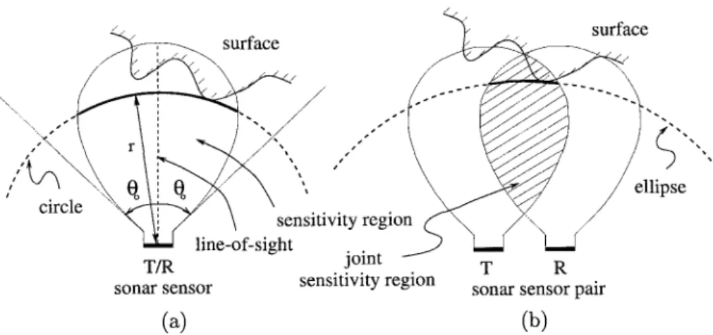
The major limitation of sonar sensors comes from their large beamwidth, as we have seen in previous chapters. Although these devices return ac-curate range data, they cannot provide direct information on the angular position of the object from which the reflection was obtained. Thus, all that is known is that the reflection point lies on a circular arc whose radius is determined by r = ct0/2 as illustrated in Fig. 7.1(a). More generally, when
one sensor transmits and another receives, it is known that the reflection point lies on the arc of an ellipse whose focal points are the transmitting and receiving transducers (Fig. 7.1(b)). Note that the reflecting surface is tangent to these arcs at the actual point (s) of reflection. The angular extent of these arcs is determined by the sensitivity regions of the transducers.
If multiple echoes are detected for the same transmitting/receiving pair, circular or elliptical arcs are constructed to correspond to each echo . (How-ever, not all systems commonly in use are able to detect echoes beyond the first one.)
Most commonly, the large beamwidth of the transducer is accepted as a device limitation which determines the angular resolving power of the system. In this naive approach, a range reading of r from a transmit-ting/receiving transducer is taken to imply that an object lies along the line-of-sight of the transducer at the measured range. Consequently, the an-gular resolution of the surface profile measurement is limited by the rather
surface surface sensitivity region line-of-sight T/R sonar sensor (a) joint sensitivity region ellipse T R sonar sensor pair
(b)
Fig. 7.1 (a) For the same sonar transmitting and receiving, the reflecting point is known to be on the circular arc shown, (b) The elliptical arc if the wave is transmitted and received by different sensors. The intersection of the individual sensitivity regions serves as a reasonable approximation to the joint sensitivity region
large beamwidth, which is a major disadvantage. Our approach, as will be seen, turns this disadvantage into an advantage. Instead of restricting oneself to an angular resolution equal to the beamwidth by representing the reflection point as a coarse sample along the line-of-sight, circular or ellip-tical arcs representing the uncertainty of the object location are drawn. By combining the information inherent in a large number of such arcs, angular resolution far exceeding the beamwidth of the transducer is obtained.
7.3 Processing of the Sonar Data
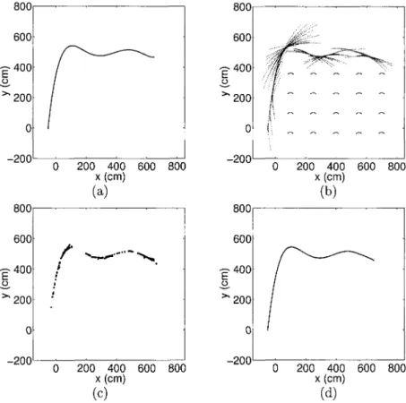
Structured configurations such as linear and circular arrays as well as ir-regular sensor configurations have been considered (The mobile robot used in the experiments has a circular array of sonar sensors.) Figure 7.2(a) shows a surface whose profile is to be determined. Part (b) of the same figure shows the circular and elliptical arcs obtained from circular arrays of sensors, which both rotate and translate to increase the number of arcs gen-erated from the available number of sensors. Further sonar maps obtained using a circular configuration are presented later in Sec. 7.3.3.2.
Notice that although each arc represents considerable uncertainty as to the angular position of the reflection point, one can almost extract the actual curve shown in Fig. 7.2(a) by visually examining the arc map in
800 800 200 400 600 800 x (cm) (a) 200 400 600 800 x (cm) (b) 800 800 -200 200 400 600 800 x (cm) (c) 200 400 600 800 x (cm) (d)
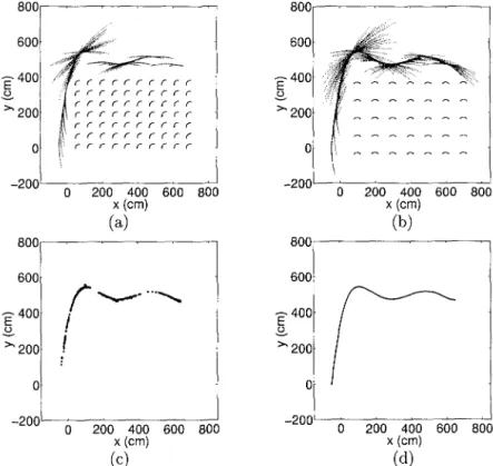
Fig. 7.2 (a) The original surface, (b) The circular sensor array mounted on a mobile robot moves to 20 different locations and collects data by rotating around its center from 45° to 135° in 15° steps. The angles are measured with respect to the positive x axis in the counterclockwise direction. The circular array has been shown at the 20 locations at its 90° position, (c) Result of n = 3 thinning: e = 0.052, fc = 0.341, tCp u - 1.11 s.
(d) The original surface (dashed line) and the polynomial fit of order m = 9 (solid line), with E\ = 3.18 cm and E2 = 0.036. In this case both coincide
Fig. 7.2(b). Each arc drawn is expected to be tangential to the surface at least at one point. At these actual reflection point(s), several arcs will intersect with small angles at nearby points on the surface. The many small segments of the arcs superimposed in this manner create the darker features in Fig. 7.2(b), which tend to cover and reveal the actual surface. The remaining parts of the arcs, not actually corresponding to any reflections and simply representing the angular uncertainty of the sensors, remain more sparse and isolated.
Morphological processing will be employed to achieve what is natural for the human visual perception system: the extraction of Fig. 7.2(a) from 7.2(b). Morphological erosion and dilation operators will be used to weed out the sparse arc segments, leaving us with the mutually reinforcing seg-ments which will reveal the original surface.
7.3.1 Morphological Processing
The main application of morphological operations is in modifying regions and shapes of images [Low 96]. Therefore, they are widely used in im-age processing to accomplish tasks such as edge detection, enhancement, smoothing, and noise removal [Dougherty 92; Myler and Weeks 93]. In this study, morphological processing is used to eliminate the sparse and isolated spikes and segments in the sonar arc map, directly revealing the surface profile.
Erosion and dilation are the two fundamental morphological operations
used to thin or fatten an image respectively. These operations are defined according to a structuring element or template. The algorithm for erosion is as follows: The template is shifted over the pixels of the sonar map which take the value 1 one at a time and the template's pixels are compared with those pixels which overlap with the template [Pitas 93]. If they are all identical, the central pixel with value 1 will preserve its value; otherwise it is set to zero.
The dilation algorithm is very similar to that for erosion, but it is used to enlarge the image according to the template. This time, all eight neighbours of those image pixels which originally equal 1 are set equal to 1.
In this study, the structuring element for dilation and erosion is chosen to be a 3 x 3 square template. Since the template is symmetric, the image will be fattened (dilation) or thinned (erosion) in all directions by one pixel. The direct use of erosion may eliminate too many points and result in the loss of information characterising the surface. For such cases, the com-pound operations of opening and closing are considered. Opening consists of erosion followed by dilation and vice versa for closing. Opening helps reduce small extrusions, whereas closing enables one to fill the small holes in the image [Myler and Weeks 93]. Closing is applied prior to thinning, described below, in cases where the points are not closely connected to each other so that the direct use of thinning may result in the loss of too many points. Filling the gaps using closing first may prevent this from happening.
Thinning is a generalisation of erosion with a parameter n varying in
the range 1 < n < 8. In this case, it is sufficient for any n neighbours of the central image pixel to equal 1 in order for that pixel to preserve its value of 1. The flexibility that comes with this parameter enables one to make more efficient use of the information contained in the arc map.
In pruning, which is a special case of thinning, at least one (n = 1) of the neighbouring pixels must have the value 1 in order for the central pixel to remain equal to 1 after the operation. This operation is used to eliminate isolated points [Dougherty 92]. Thus, pruning and erosion are the two extremes of thinning with n = 1 and n = 8 respectively.
Since there are many alternatives for morphological processing of sonar data, an error measure is introduced as a success criterion:
e — [i A)
Here, i is the discrete index along the x direction and yi is the discretised function representing the actual surface profile with variance
ay = ~k 2j=i(y» — ~k ^2iVi)2- N is the total number of columns whereas
Nk represents those columns left with at least one point as a result of some
morphological operation, rrii is the vertical position of the median (center-most) point along the ith column of the map matrix (e.g. Fig. 7.2(c)). If there are no points in a particular column, that column is excluded from the summation. If the number of columns thus excluded is large; that is, if the morphological operations have eliminated too many points, the re-maining points will not be sufficient to extract the contour reliably, even if e is small. We will denote by fc = Nk/N the fraction of columns left
with at least one point at the end of a morphological operation. This factor must also be taken into account when deciding on which method provides a better result.
Additionally, the CPU times of the algorithms (iCpu) are measured.
These represent the total time the computer takes to realise the morpholog-ical operations starting with the raw TOF data. Morphologmorpholog-ical operations are implemented in the C programming language and the programs are run on a 200 MHz Pentium Pro PC.
The result of applying n — 3 thinning to the sonar arc map shown in Fig. 7.2(b) is presented in part (c) of the same figure and the results of various morphological operators applied to the same map are summarised
morphological operatior I thinning (n = 1 : pruning) thinning (n = 2) thinning (n = 3) thinning (n = 4) thinning (n = 5) thinning (n = 6) thinning (n = 7) thinning (n = 8 : erosion) closing & thinning (n = closing & thinning (n =
3) 4) e 0.168 0.074 0.052 0.045 0.012 0.014 0.007 — 0.121 0.122 fc 0.924 0.637 0.341 0.160 0.063 0.021 0.003 0.000 0.760 0.641 Ex (cm) 7.83 4.42 3.18 5.37 16.21 464.30 1915.45 — 6.72 6.88 Ei 0.089 0.050 0.036 0.061 0.183 5.246 21.641 — 0.076 0.078 I C P U (,Sj 1.15 1.12 1.11 1.10 1.09 1.10 1.10 1.10 7.10 7.09 Table 7.1 Results of various morphological operations and curve fitting of order m = 9. Since fc = 0 for n = 8 thinning, reflecting the fact that all points are eliminated, the
values of e, E\, and £ 2 are undefined for this case
in Table 7.1. Error measures E\ and E2, given in the same table, will
be defined and discussed later in Sec. 7.3.2. Since simple erosion results in very small values of fc, we have considered thinning with parameter n.
The error e tends to decrease with increasing n. However, larger values of
n tend to result in smaller values of fc so that a compromise is necessary.
For the time being, we note that the thinning parameter n allows one to trade off between e and fc.
7.3.2 Curve Fitting
As a last step, curve fitting is applied in order to achieve a compact rep-resentation of the surface profile in the robot's memory. Since our aim is to fit the best curve to the points, not necessarily passing through all of them, least-squares optimisation (LSO) is preferred to interpolation. LSO finds the coefficients of the best-fitting polynomial p(x) of order m (which is predetermined) by minimising
N Mi
S
p
2= E E b f e ) - / i / (7-2)
1 = 1 j=l
where E% is the sum of the squared deviations of the polynomial values p{xi) from the data points / y . Xi is the horizontal coordinate corresponding to the ith column of the map matrix and / y is the vertical coordinate
of the jth point along the ith column. The index j runs through the
Mi points along column i, and N is the number of columns. If M$ = 0
for a certain column, the inner summation is not evaluated and taken as zero for that column. The coefficients of the polynomial are determined by solving the linear equations obtained by setting the partial derivatives equal to zero [Lancaster 86]. Once an acceptable polynomial approximation is found, the surface can then be represented compactly by storing only the coefficients of the polynomial. Although polynomial fitting has been found to be satisfactory in all of the cases considered, other curve representation approaches such as the use of splines might be considered as alternatives to polynomial fitting.
To assess the overall performance of the method, two final error mea-sures are introduced, both comparing the final polynomial fit with the ac-tual surface: Ex =
i
\f^Wi)-Vi? (7-3) i = l E, E2 = — (7.4) (TyThe first is a root-mean-square absolute error measure, with dimensions of length, which should be interpreted either with respect to the pixel size, or with respect to the wavelength A, which serves as a natural reference for the intrinsic resolving power of the system. The second is a dimensionless relative error measure which can be interpreted as the error relative to the variation of the actual surface.
The curve fitted to the surface map after the thinning shown in Fig. 7.2(c) is presented in part (d) of the same figure. Table 7.1 shows that increasing
n improves e but worsens fc and that E\ and E2 achieve a minimum at
some value of n (which in this case happens to occur at n = 3 for both E\ and E2). In the simulations, where the actual surface is known, it is
possi-ble to choose the optimal value of n, minimising E\ or E2. In real practice,
this is not possible so that one must use a value of n judged appropriate for the class of surfaces under investigation.
In the simulations, higher-order reflections* are ignored since they are *A higher-order reflection refers to an echo detected after bouncing off from object
surfaces more than once.
difficult to model, although they almost always exist in practice: The key idea of the method is that a large number of data points coincide with the actual surface (at least at the tangent points of the arcs) and the data points off the actual curve are more sparse. Those spurious arcs caused by higher-order reflections and crosstalk also remain sparse and lack reinforce-ment most of the time. The thinning algorithms eliminate these spurious arcs together with the sparse arc segments resulting from the angular un-certainty of the sensors.
7.3.3 Simulation Results
The approach taken in this paper is very general in that arbitrary con-figurations and orientations of sensors can be handled equally effectively. We begin by considering the special cases of linear and circular arrays, which might be typical of deliberately designed array structures. Following these, we also consider arrays where the sensors are situated and oriented randomly. This not only exemplifies the general case where the array struc-ture is irregular, but might also have several applications: For instance, it may correspond to the case where arcs are accumulated by any number of randomly moving and rotating sensors, perhaps mounted on mobile robots as in swarm robot applications. Another potential area of application of the random configuration is in array signal processing where the individ-ual sensor positions of a regular array have been perturbed by the wind or waves.
7.3.3.1 Linear Arrays
First, linearly configured sensor arrays were considered. Given the beamwidth of the sensors (25°), it was observed that the number of arcs collected is relatively small. The situation gets even worse as the array is brought closer to the surface since interaction between an even smaller number of sensor pairs becomes possible. This is a consequence of the fact that the angular beamwidth subtends a smaller arc on the surface. It is interest-ing to note that whereas narrow beamwidths are esteemed for their high resolving power in conventional usage of such sonar sensors, here it would have been desirable to have sensors with larger beamwidths. This would enable a greater number of sensor pairs to produce a greater number of elliptical arcs, better and faster revealing the surface. However, since we
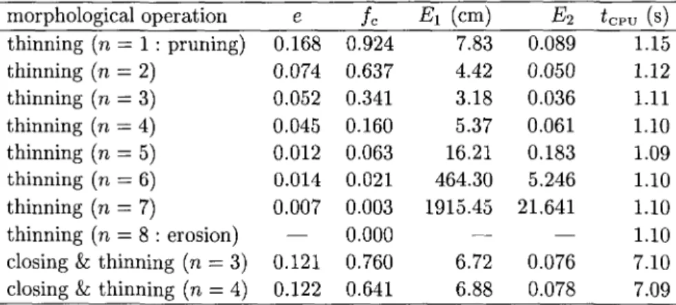
restrict ourselves to the parameters of the most widely available transducer (i.e. the Polaroid), rotating the sensors is considered instead to make up for their limited beamwidth, as shown in Figs. 7.3(a) and (b).
A further consideration is that in practice the number of sensors may be limited. One way to overcome this limitation is to move a smaller array much in the same spirit as synthetic aperture radar (SAR) techniques [Skol-nik 81]. However, this is not completely equivalent to the full array since those elliptical arcs corresponding to pairs of sensors not contained within the actually existing array are missing. A further extension is the combi-nation of such movement and rotation as was the case in our first example in Fig. 7.2.
We now return to Figs. 7.3(a) and (b) where the sensors are not trans-lated but are only rotated. The results of morphological processing are presented in parts (c) and (d), and the curves fitted to them are shown in parts (e) and (f) of the same figure. In these and later simulations, the values of n and m chosen are those which give the smallest error E\, unless otherwise indicated.
7.3.3.2 Circular Arrays
The circular configuration corresponds to the arrangement of sonar sensors on the Nomad 200 mobile robot in our laboratory. Only the five sensors fac-ing the surface are activated since the others cannot see the surface. Again, the surface shown in Fig. 7.2(a) is considered. In addition to the array locations in Fig. 7.2(b), two further examples are presented in Figs. 7.4(a) and (b). The result of applying morphological processing and curve fitting to the sonar map in part (b) is presented in parts (c) and (d) of the same figure.
7.3.3.3 Arbitrarily-Distributed Sensors
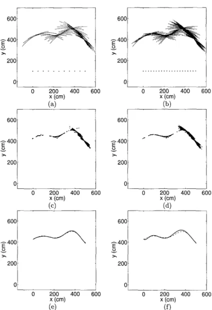
In this section, the locations and the line-of-sight orientations of the sensors are generated randomly and do not conform to any special structure. In Fig. 7.5(a), a surface is shown whose profile is to be determined with such a configuration. Parts (b) and (c) show the sonar arcs obtained using different numbers of sensors. In Fig. 7.6(a), the surface features obtained after applying n = 2 thinning to the sonar arcs in Fig. 7.5(b) is shown. Similarly, applying n = 5 thinning to the arc map in Fig. 7.5(c), the result in Fig. 7.6(b) is obtained. The curves fitted to the surface features extracted
600 ^400 200 0 200 400 600 x (cm) (a) 600 400 200 200 400 x (cm) (c) 600 600 :-400 200 200 400 x (cm) (e) 600 600 -400 200 600 ,400 200 600 ,400 200 0 200 400 600 x (cm) (b) 200 400 x (cm) (d) 600 200 400 x (cm) (f) 600
Fig. 7.3 Two linear arrays where the sensors are individually rotated from 40° to 140° in 10° steps: (a) An array of 11 sensors with 50 cm spacing, (b) An array of 21 sensors with 25 cm spacing, (c) Result of closing and n = 5 thinning applied to part (a): e = 0.276, fc = 0.772, tCpu = 4.51 s. (d) Result of n = 3 thinning applied to part (b):
e = 0.353, /c = 0.864, <CPU = 1-28 s. (e) Polynomial fit of order m = 8 to part (c) (solid
line), and the actual surface (dashed line). E\ = 3.03 cm, Ei = 0.127. (f) Polynomial fit of order m = 7 to part (d), and the actual surface. E\ = 7.85 cm, Ei = 0.329
-200 -200 0 200 400 600 800 x (cm) (a) 200 400 600 800 x (cm) (c) -200 0 200 400 600 800 x (cm) (b) 200 400 600 800 x (cm) (d)
Fig. 7.4 (a) The robot is located at 70 locations and the front sonar is oriented at 135° with respect to the positive x axis. No rotation, (b) The robot rotates at 35 locations, from 45° to 135° in 15° steps, (c) Result of n = 5 thinning applied to part (b): e = 0.050, fc = 0.464. (d) Polynomial fit of order m = 11 (solid line) and the actual surface (dashed
line). Ei = 3.57 cm, E2 = 0.040. In this case both coincide
are presented in parts (c) and (d) of the same figure.
Although structured arrays such as linear or circular ones are often preferred in theoretical work for simplicity and ease of analysis, the method presented here is capable of equally easily handling arbitrary arrays. In fact, the large number of simulations we have undertaken indicate that arrays consisting of irregularly located and oriented sensors tend to yield better results. This seems to result from the fact that the many different vantage points and orientations of the sensors tend to complement each other better than in the case of a uniform array. Although the question of optimal complementary sensor placement is a subject for future research,
200 400 x (cm) (a) 200 400 x (cm) (c)
Fig. 7.5 (a) The original surface, (b) The arcs corresponding to the sonar T O F d a t a collected from the surface using 100 sensors scattered and oriented randomly (not shown). The x and y coordinates of each sensor are independent and uniformly distributed in the intervals [0,500] and [0,360] respectively. The orientation is uniformly distributed in [40°, 140°]. (c) 150 sensors are used (not shown)
the results imply that it is preferable to work with irregular or randomised arrays rather than simple-structured arrays such as linear or circular ones.
7.4 Experimental Verification
In this section, the method is verified using the sensor systems on the Nomad 200 mobile robot in our laboratory.
7.4.1 System Description
The Nomad 200 mobile robot, shown in Fig. 7.7, has been used in the ex-periments. It is an integrated mobile robot including tactile, infrared, sonar and structured-light sensing systems, with dimensions 76.2 cm (height) and 45 cm (diameter). The mechanical system of the robot uses a non-holonomic, three-servo, three-wheel synchronous drive with zero gyro-radius. The control of the base translation, base rotation and turret rotation is performed by three separate motors. The robot can translate only in the forward and backward directions but not sideways without rotating first. Servo control is achieved by a MC68008/ASIC microprocessor system. The maximum translational and rotational speeds of the Nomad 200 are 60 cm/s and 60° / s respectively. Nomad 200 has an on-board computer for sensor and motor control and for host computer communication. The communi-cation is managed with a radio link and a graphics interface (server). The robot can be run from a C-language program either through the server or
200 400 x (cm) (a) 600 200 400 x (cm) (b) 600 600 ^400 200 200 400 x (cm) 600 200 400 x(cm) 600 (d)
Fig. 7.6 (a) Result of n = 2 thinning applied to Fig. 1.5(b): e = 0.296, fc = 0.566,
tCpv = 0.49 s. (b) Result of n = 5 thinning applied to Fig. 1.5(c): e = 0.133, fc = 0.610,
tcpu = 0.73 s. (c) Polynomial fit of order m = 6 to part (a) (solid line), and the actual surface (dashed line). E\ = 3.92 cm, E2 = 0.164. (d) Polynomial fit of order m — 6 to part (b) (solid line), and the actual surface (dashed line). E\ = 2.30 cm, £ 2 = 0.090
directly.
We next give a brief description of the two sensor modules used in the experiments:
The Sensus 200 Sonar Ranging System consists of 16 sonars which can yield range information from 15 cm to 10.7 m with ± 1 % accuracy. The sensors are Polaroid 6500 series transducers [Polaroid 97] which determine the range by measuring the TOF. The transducer beamwidth is 25°. The carrier frequency of the emitted pulses is 49.4 kHz. The system can be interfaced with any type of microcontroller. The power requirements of the system are 100 mA at 5 V or 12 V [Nomad 97].
Fig. 7.7 Nomad 200 mobile robot. The ring of sonars can be seen close to the top rim of the turret, and the structured-light system is seen pointing rightwards on top.
The Sensus 500 Structured-Light System basically consists of a laser diode (as its light source) and a CCD array camera. The laser beam is passed through a cylindrical lens in order to obtain planar light. The op-erating range of the system is from 30.5 cm to 3.05 m. Within this range, the intersection of the plane of light with the objects in the environment can be detected by the camera. The range is determined by (laser line striping) triangulation, characterised by decreasing accuracy with increas-ing range.[Everett 85]. The power requirement of the system is 2000 mA at 12 V [Nomad 97].
In the experiments, both sonar and structured-light data are collected from various surfaces constructed in our laboratory. The structured-light system is much more expensive and complex, requiring higher-power and sufficient ambient light for operation. Since it reveals a very accurate sur-face profile, the sursur-face detected by this system is used as a reference in the experiments.
In order to prevent any crosstalk between consecutive pulses, the sonars should be fired at 62 ms intervals since the maximum range of operation of Polaroid transducers is 10.7 m. In the experiments, the sonars are fired at
40 ms intervals. This prevents much of the crosstalk, and in the few cases where erroneous readings are obtained due to crosstalk, these false readings are readily eliminated by the algorithm. This is another aspect in which the algorithm exhibits its robust character.
-foo -50 0 50 100 x{cm) 150 E" a.100 50 (a) .r -*+: ^% -TOO - 5 0 0 50 100 x (cm) (c)
Fig. 7.8 (a) The surface profile revealed by the structured-light data, (b) the sonar data. The data in both parts are collected from the surface at every 2.5 cm by translating the mobile robot from ( — 75,0) to (75,0). (c) Result of erosion (n = 8) followed by pruning (n = 1). (d) Polynomial fit of order m = 10. (e) Part (a) superimposed with part (d) to demonstrate the fit obtained. E\ = 3.59 cm, E2 = 0,263, and i c p u — 0.27 s
7.4.2 Experimental Results
The sonars on the Nomad 200 are in a circular configuration. Since the robot has a limited number of sensors which can detect the surface, by moving the robot and rotating its turret, the equivalent of a much larger number of sensors is created synthetically. First, the robot remained sta-tionary and collected data by rotating its turret. However, there were many locations on the surface which could not be detected by the robot if only the turret rotated. On the contrary, pure translation alongside the surface generally provided satisfactory results.
First, several surfaces have been constructed in our laboratory with different curvature and dimensions, using thin cardboard of height 1.05 m and length 3.65 m. In these experiments, only the front five sensors have been activated.
The structured-light data obtained from one of the cardboard surfaces constructed are presented in Fig. 7.8(a). The sonar data presented in Fig. 7.8(b) are obtained by translating the mobile robot horizontally over a distance of 1.5 m along the line y = 0 and collecting data every 2.5 cm. The turret is oriented such that both the structured-light and the front five sonars are directed towards the surface and it does not rotate throughout the translational movement.
If the sonar data in Fig. 7.8(b) are examined, it can be observed that there are many points on the surface which have not been detected by the sonars. Since the reflections are specular, segments of the surface which are relatively perpendicular to the transducer line-of-sights are easily detected, whereas those segments which are more or less aligned with the line-of-sights could not be sensed.t This is less of a problem when the surface is relatively smooth and its curvature is small. The extent to which this becomes a problem depends on the radius of curvature, as will be evident when we consider below a second example with less curvature.
As expected, the structured-light data provide a very accurate surface profile. In the arc map obtained by sonar, there are some arcs which are not tangent to the actual surface at any point (e.g. the isolated arcs in the upper right and upper left parts of Fig. 7.8(b)). These correspond to spurious data due to higher-order reflections, readings from other objects in the environment, or totally erroneous readings. These points are readily eliminated by the morphological processing (Fig. 7.8(c)). If the final curve in Fig 7.8(d) is compared with the structured-light data (Fig. 7.8(e)), it can be observed that a close fit to the original surface is obtained. The errors in this case are E\ = 3.59 cm, E2 = 0.263, and the CPU time is tCPU = 0.27 s.
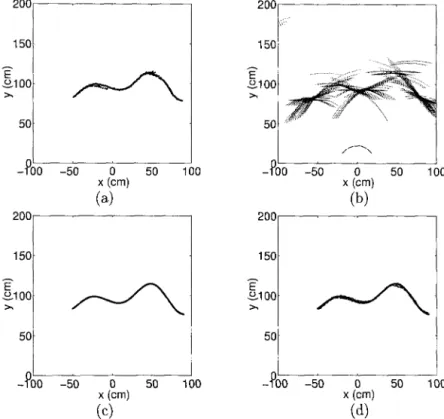
Next, a surface with smaller maximum curvature (hence with larger min-imum radius of curvature), shown in Fig. 7.9(a), is considered. The results of morphological processing and curve fitting are shown in Fig. 7.9(c)-(e), tSince specular reflections involve negligible scattering and mirror-like reflections, the transmitted waveform can be received back at the transducer only if some of the rays emerging from the transducer are perpendicular to the surface. For the case of separate transmitter and receiver, the surface must be perpendicular to the normal determined by the transmitting and receiving elements.
200 200 TOO - 5 0 0 50 100 x (cm) (a) 200 TOO -50 0 50 100 x (cm) (b) 200 100
Fig. 7.9 (a) T h e surface profile revealed by the structured-light data, (b) the sonar data. T h e data in both parts are collected from the surface at every 2.5 cm by translating the mobile robot from ( - 7 5 , 0 ) to (75,0). (c) Result of erosion (n = 8) followed by pruning (n = 1). (d) Polynomial fit of order m = 10 to part (a), (e) Part (a) superimposed with part (d) to demonstrate the fit obtained. E\ = 1.41 cm, E2 = 0.156, and iCp u = 0.39 s
resulting in Ex = 1.41 cm, E2 = 0.156 and tCTV = 0.39 s. It is indeed
observed that Ex and E2 are reduced significantly with respect to the
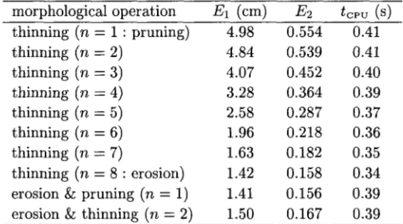
pre-vious case, as also evidenced by the much better fit seen in Fig. 7.9(e). Several results obtained for this surface are summarised in Table 7.2. All polynomials are of degree m = 10. The minimum estimation error Ei is not much larger than the wavelength A = 6.9 mm.
It is worth noting that the present approach is aimed at estimation of a curve, as opposed to detection of target primitives. When corners or edges are encountered in the environment, the method does not fail but the results slightly deteriorate since the method exploits neighbouring
morphological operation thinning (n = 1 : pruning) thinning (n = 2) thinning (n = 3) thinning (n = 4) thinning (n = 5) thinning (n = 6) thinning (n = 7) thinning (n = 8 : erosion) erosion & pruning (n = 1) erosion & thinning (n = 2)
Ei (cm) 4.98 4.84 4.07 3.28 2.58 1.96 1.63 1.42 1.41 1.50 E2 0.554 0.539 0.452 0.364 0.287 0.218 0.182 0.158 0.156 0.167 ' C P U (SJ 0.41 0.41 0.40 0.39 0.37 0.36 0.35 0.34 0.39 0.39
Table 7.2 Experimental results for the surface given in Fig. 1.9(a) for different morpho-logical operations.
Fig. 7.10 In all three parts, the result of curve fitting (solid line) is compared to the original surface profile as revealed by t h e structured-light data. D a t a are collected by rotating the turret of the robot from —30° to 30° taking 1° steps, (a) 90° corner at 80 cm: polynomial fit of order m = 6, resulting in E i = 1.90 cm and Ei = 0.217. (b) 60° corner at 80 cm: polynomial fit of order m = 10, resulting in E\ = 1.96 cm and E2 = 0.243. (c) 90° edge at 60 cm: polynomial fit of order m = 8 resulting in
Ei - 3.83 cm and E2 = 0.414
relationships and local continuity (i.e. smoothness). Experimental results for 60°, 90° corners and 90° edge are presented in Fig. 7.10. These objects are made of smooth wood and are 1.20 m in height. The results indicate that the method works acceptably in such cases as well, the net effect being that the vertices of the sharp edges are rounded or smoothed (i.e. low-pass filtered) into curved edges. This corresponds to the spatial frequency resolving power of the system as determined by the chosen grid spacing.
200 100 . 0 -100 -200 l I -200 -100 0 100 200 x (cm) (a) -200 -100 0 100 200 x (cm) (b) 200 100 f 3. 0 >> -100 -200 ^ - —>>•
'-f
-200 -100 0 100 200 x (cm) (c)Fig. 7.11 (a) Structured-light d a t a collected from a room comprised of planar walls, corners, an edge, a cylinder, and a doorway, (b) Sonar arc map and the robot's path. (c) The result of n = 3 thinning
Finally, we present experimental results obtained by using the front three sonars of the Nomad 200 robot, following the walls of the room in Fig. 7.11(a). The room comprises of smooth wooden (top and left) and plas-tered (right) walls, and a window shade with vertical flaps of 15 cm width (bottom). Some of the corners of the room were not perfect (e.g. where the shade and the right wall make a corner). A cylindrical object of radius 15 cm is present at a distance of 30 cm from the center of the right wall. In Fig. 7.11(b), the path of the robot and the resulting arc map are given. In Fig. 7.11(c), the result of morphological processing is shown. It is clear from this figure that despite the potential for many higher-order reflections, spurious arc segments have been fairly well eliminated, and we can expect a good polar polynomial fit (or line segment matching).
Even though the method was initially developed and demonstrated for specularly reflecting surfaces, subsequent tests with Lambertian surfaces of varying roughness have indicated that the method also works for rough sur-faces, with errors slightly increasing with roughness [Barshan and Baskent 00].
Closing operations were not needed in processing the experimental data because the points were sufficiently dense. If this was not the case, one would first apply closing in order to add extra points to fill the gaps between the points of the original map.
7.4.3 Computational Cost of the Method
The average CPU times are in general of the order of several seconds, indi-cating that the method is viable for real-time applications. These represent the total time the computer takes to realise the morphological operations starting with the raw TOF data. (The morphological processing has been implemented in C language and runs on a 200 MHz Pentium Pro PC.) For comparison, the time it takes for an array of 16 sonars to collect all the TOF data is 16 x 40 ms = 0.64 s which is of the same order of magnitude as the processing time. It should be noted that the actual algorithmic pro-cessing time is a small fraction of the CPU time, as most of the CPU time is consumed by file operations, reads and writes to disk, matrix allocations etc. Thus, it seems possible that a dedicated system can determine the surface profile even faster, bringing the computation time below the data collection time.
Another important factor is memory usage. In the simulations, the objects are relatively large and a relatively large number of sensors are employed. This leads to memory usage ranging between 100-750 kB. In the experiments, the targets are smaller and relatively close so that the data files consume about 50-100 kB. Although memory usage depends on the number of sensors used, size of the object, and the grid size, these figures are representative of the memory requirements of the method.
7.5 Discussion and Conclusions
A novel method is described for determining arbitrary surface profiles by applying morphological processing techniques to sonar data. The method is both extremely flexible, versatile, and robust, as well as being simple and straightforward. It can deal with arbitrary numbers and configurations of sensors as well as synthetic arrays obtained by moving a relatively small number of sensors. Accuracy increases with the number of sensors used (actual or synthetic) and has been observed to be quite satisfactory. The method is robust in many aspects; it has been seen that it has the inher-ent ability to eliminate most of the undesired TOF readings arising from higher-order reflections as well as the ability to suppress crosstalk when the sensors are fired at shorter intervals than that nominally required to avoid crosstalk. In addition, the method can effectively eliminate spurious TOF measurements due to noise, and process multiple echoes informatively.
The processing time is small enough to make real-time applications fea-sible. For instance, the system can be used for continual real-time map building purposes on a robot navigating in an environment with vertical walls of arbitrary curvature. Two extensions immediately come to mind: First, it is possible for the robot to continually add to and update its col-lection of arcs and reprocess them as it moves, effectively resulting in a synthetic array with more sensors than the robot actually has. Second, the method can be readily generalised to three-dimensional environments with the arcs being replaced by spherical or elliptical caps and the morphological rules extended to three dimensions. The method was also found successful in determining the profile of surfaces completely surrounding the sensing system. In this case, it may be preferable to reformulate the method in polar or spherical coordinates.
Although the structured-light system has been used mainly as a refer-ence in this study, the fact that its strengths and weaknesses are comple-mentary to the sonar system suggests the possibility of fusing the output of the two systems. The structured-light system provides a very accurate sur-face profile, but introduces errors increasing with range, as a result of the triangulation technique it employs. On the other hand, sonars yield bet-ter range information over a wider range of operation, but are less adept at recognising the contour details due to their wide beamwidth. Despite the possibility of fusion, the method described in this paper may be prefer-able in many circumstances, since the structured-light system is much more expensive and complex compared to sonar sensors.
Although not fully reported here, a detailed quantitative study of the performance of different morphological operations and the dependence of the error on surface curvature, spatial frequency, distance, sensor beamwidth, and TOF noise can be found in [Barshan and Baskent 01]. In [Barshan and Baskent 00], processing the arc maps using morphological processing is compared to using spatial voting instead.
The essential idea of this chapter—the use of multiple range sensors combined with morphological processing for the extraction of the surface profile—can also be applied to other physical modalities of range finding of vastly different scales and in many different application areas. These may include radar, underwater sonar, optical sensing and metrology, remote sensing, ocean surface exploration, geophysical exploration, and acoustic microscopy. Some of these applications (e.g. geophysical exploration) may involve an inhomogeneous and/or anisotropic medium of propagation. It is
envisioned that the method could be generalised to this case by constructing broken or non-ellipsoidal arcs.
Acknowledgment
This work has been adapted from [Baskent and Barshan 99] (©1999 Sage Publications, Inc.). The authors are grateful for the support of TUBITAK under grant 197E051.