A simulation program for efficient analysis of linear circuits

τ κ i f S J t .

‘S è ê

tsas

I SiaGLÄT’Ü;! ? 3 S S M fM !?nS!EI?

P i . V îJî BF n i ï ? s ί·;|·

5

- ^ '·

O^îûl! s!?®* '..'N_{•«D V i'i^‘»! 1.И i*Vi}

Tr-C FicCiÜ·FC£^>:İ :»OTC»·^*^ гѵ'

A SIMULATION PROGRAM FOR EFFICIENT

ANALYSIS OE LINEAR CIRCUITS

A THESIS

SUBMITTED TO THE DEPARTMENT OF ELECTRICAL AND ELECTRONICS ENGINEERING

AND THE INSTITUTE OF ENGINEERING AND SCIENCES OF BILKENT UNIVERSITY

IN PARTIAL FULFILLMENT OF THE REQUIREMENTS FOR THE DEGREE OF

MASTER OF SCIENCE

By

Mustafa Simgiir

September 1996

т к 4 5 4

• 5 â é

I certify that I have read this thesis and that in my opinion it is fully adequate, in scope and in quality, as a thesis for the degree of Master of Science.

l ·

Prof. Dr. Abdullah Atalar(Supervisor)

I certify that I have read this thesis and that in my opinion it is fully adequate, in scope and in quality, as a thesis for the degree of Master of Science.

Assoc. Prof. Dr. M. İrşadi Aksun

I certify that I have read this thesis and that in my opinion it is fully adequate, in scope and in quality, as a thesis for the degree of Master of Science.

Assoc. P > C T r . Cevdet Aykanat

Approved for the Institute of Engineering and Sciences:

Prof. Dr. Mehmet Bat

Director of Institute of EngineeriH^ and Sciences

ABSTRACT

A SIMULATION PROGRAM FOR EFFICIENT ANALYSIS

OF LINEAR CIRCUITS

Mustafa Sungur

M.S. in Electrical ¿ind Electronics Engineering

Supervisor: Prof. Dr. Abdullah Atalar

September 1996

A circuit simulation program using generalized asymptotic waveform evalua­ tion technique is introduced. The program analyzes circuits with lumped a.nd distributed components. It computes the moments ci.t a few Irecjuency points and extracts the coefficients of an approximating rational by employing one of t,he two different methods. One of the examined methods is proposed to compare the accuracy of results and the execution times with conventional simulators and sevei’cil examples are demonstrated, indicating that our sirnulcv tor provides a. speed improvement without a significant loss of accura.cy.

Keywords : Circuit Simulation, Asymptotic Waveform Evahuition, Multi point

Fade Approximation, AC Analysis, MAWE, Spice, Computer Aided Design, CAD

ÖZET

LİNEER DEVRELERİN VERİMLİ ANALİZİ İÇİN BİR

BENZETİM PROGRAMI

Mustafa Sungur

Elektrik ve Elektronik Mühendisliği Bölümü Yüksek Lisans

Tez Yöneticisi: Prof. Dr. Abdullah Atalar

Eylül 1996

Genelleştirilmiş asimtotik clalgaşekli hesaplaması tekniğini kullanan bir devre benzetim programı sunulmuştur. Program, dağılmış ve ortak parametreli de­ vrelerin analizini yapar. Bu program, devrenin momentlerini birkaç frekans noktasında hesaplar ve kesirli yaklaşım fonksiyoriunun katsayılarını anlatılan iki m etottan birisini kullanarak ortaya çıkarır. Denenen metotlardan biri, sonuçların doğruluğu ve çalışma zamanı l^akımmdan bilinen benzetim pi’o- gramları ile karşıhıştırmak için önerilmiş ve bizim benzetim programımızın doğruluğundan birşey kaybetmeden, zamanda iyileştirme yaptığını gösteren bazı örnekler verilmiştir.

AnaJıtar Kelimeler : Devre Benzetimi, Asimtotik Dalgaşekli Hesaplama, Çok

noktalı Pade Yaklaşımı, AC Analiz, MAWE, Spice, Bilgisayar Destekli 'J aşarim, CAD

ACKNOWLEDGEMENT

I would like to express my deep gratitude to rriy supervisor Dr. Abdullah Atalar for his supervision, guidance and suggestions throughout the develop­ ment of this work.

I would like to thank A. Suat Ekinci for his colloboration, numerous sug­ gestions and invaluable help. I would also like to thank previous members of the CAD group at Bilkent University; Mustafa Yazgan, Ogan Ocali, Mustafa Çelik and Satılmış Topçu for their useful previous work.

TABLE OF C O N T E N T S

1 IN T R O D U C T IO N 1

2 A SY M PT O T IC WAVEFORM EVALUATION 3

2.1 Linear Circuits and AWE 3 2.2 Computation of m om ents... 4

2.3 Order Reduction .5

3 M ULTI PO IN T PADE APPRO XIM A TIO N 7

3.1 Frequency Shifted M o m e n ts ... 7 3.2 Multi point Moment M atching... 8

3.2.1 Method I 9

3.2.2 Method I I ... 11 3.3 Complex Frequency H opping... 1.3

4 M O M EN T G ENERATIO N 15

4.1 Linear Circuit Form ulation... 15

4.2 Evaluation of Monient.s... 17

4.2.1 E xam ple... 17

I 5 COM PUTATIONAL CO N C EPTS 21 0.1 Algorithm of the sim u lato r... 21

5.1.1 Selection of the expansion points 22 5.1.2 Extracting the coefficients... 22

5.2 Numerical issues 23 5.2.1 Using high precision a r ith m e tic ... 24

5.2.2 S ta b ility ... 24 6 EXAM PLES 25 6.1 Example 1 ... 25 6.2 Example 2 ... 28 6.3 Example 3 ... 31 6.4 Example 4 ... 33 6.5 Discussion of the r e s u l t s ... 36 7 CONCLUSION 38 A P P E N D IX 39 A I/O FORMAT OF THE PR O G R A M 40 A.l Configuration File (.config)... 40

A.2 Circuit Input File (inlin.sp) 41 A.2.1 Options C a r d ... 41 A.2.2 Other C a r d s ... 12 A.3 Output of the p ro g ra m ... 43

LIST OF F IG U R E S

3.1 Pole selection algorithm in C F H ... 14

4.1 Illustrative example for moment generation... 18

4.2 Output of the one transmission line c ir c u it... 20

6.1 Example 1: Interconnect model with 7 transmission lines . . . . 26

6.2 Output waveform for the interconnect network in Ex. 1 ... 27

6.3 Run time distribution of MAW’E for Example 1 28 6.4 Example 2: Cascaded interconnects with 14 transmission lines . 28 6.5 AC Response of MAWE in cascaded interconnect circuit in Ex. 2 30 6.6 Absolute error of MAVVE response for Example 2 ... 30

6.7 Run time distribution of MAWE for Example 2 ... 31

6.8 Example 3: Lowpass filter with 5 transmission l in e s ... 32

6.9 Lowpass filter output response... 33

6.10 Distribution bars for the lowpass filter analysis by MAWE . . . 33

6.11 Topology of the rlc circuits in Ex. 4 ... 34

6.12 AC Responses of the ric circuits with 21 and 201 n o d e s ... 3-5 6.13 Run-tirne distributions of MAWE for (a)RLC20 (b)RLC200 in

E.K. 4 ... 36 6.14 Time shares of all processes in a small and a large analysis . . . 37

LIST OF TABLES

6.1 Expansion points and the moment numbers for interconnect net­ work in Ex. 1 ... 26 6.2 Timing results for the interconnect network in Ex. 1 (1 /0 times

excluded)

6.4 Timing results for cascaded interconnects in Ex. 2 (I/O times excluded)

27 6.3 Expansion points and the moment numbers for Example 2 . . . 29 31 6.-5 Expansion points and moment numbers for the filter example. . 32 6.6 Timing results for the filter in Ex. 3 (I/O times excluded) . . . . 32 6.7 Expansion points and moment numbers for (a) 21 and (b) 201

node rlc c irc u its... 34 6.8 Timing results for the rlc networks in Ex. 4 excluding I/O times 35

C hapter 1

IN T R O D U C T IO N

Accurate simulation of VLSI circuits is an expensive task for the large circuit sizes of today. With the advances in integrcited circuit technology, the physical circuit sizes are reduced and the operating speeds are increased. Shrinking device sizes and increasing operating speeds require faster circuit simulation programs which do not trade execution time for accuracy. Spice-like programs with high ciccuracy are needed for intensive verification and design of VLSI circuits, but for reducing execution times, new circuit solving cilgorithrns w(ire introduced. While Spice-like simulators predict the behiivior of the circuit at a large; number of discrete points both in frequency and time domain analysis, most of the new simulators employ faster algorithms to solve the circuit matrix at lower number of points. The drawback of these algorithms is the loss of accuracy, and the effort is to reduce the execution time without losing much a.ccuracy.

Asymptotic Waveform Eveduation (AWE) technique)!], is used in some new simulators in order to reduce the execution time of the simulation. Instead of solving the circuit at many discretized points, AWE seeks to capture the be­ havior by cvpproximating the dominant poles of the circuit with a lower order model. The reduced order model is matched to the moments of the linear circuit, which are obtained from the Taylor series expansion of the circuit re­ sponse around s = 0. Since the information carried by the moments is accurate

at low frequency region, the AWE technique will be efficient in extrcicting the low frequency poles of the circuit. At relatively higher frequencies the AWE technique becomes inefficient and several methods are proposed to improve

a w e’s accuracy. AWE is extended to handle distributed elements [2, 3] in order to analyze circuits that cannot be modeled by only lumped components. Also, Laurent series expansion (s = oo) is added to improve the ciccuracy of transient analysis in the vicinity of /; = 0 [4]. The stability of approximations is improved by manipulating the moment matching techniques [5].

Recently, the Complex Frequency Hopping technique is introduced in order to find all of the dominant poles of the circuit in a Irequency range of interest [6]. The PVL algorithm, Piide Approximation via Lanczos Process, is introduced to provide high numerical stability to the Pade Approxirnants [7].

In the x’ecent past, a multi point Pade Approximation was proposed [8] lor analysis of interconnect networks with transmission lines not only in low frequencies but also in high frequency regions. Apart from the moments cit

s = 0 (DC), this method uses shifted moments cis well. This proi^erty provides

the necessciry information about all frequency range. This approach requires the solution of the circuit matrix at several frequency points determined by the complex frequency hopping technique.

In this study, we introduce a simulation program for multi point Pade approximation of linear circuits. We compute the frequency shifted moments at several expansion points and match those to a lower order approximating ratiomil by using two methods. The program is implemented in C + + language running on UNIX and uses the moment matching algorithms given in [8]. The theoreticcil background of the work and the methods are introduced in the next 3 chapters. The methods introduced are conq^ared with Spice simulators in respect to their accuracy and execution times. Beginning from Section V, we present the simulations and computational results on severed examples to demonstrate the efficiency of the proposed simulator.

Chapter 2

A SY M P T O T IC W AVEFORM

EVALUATIO N

2.1

Linear C ircuits and AWE

The asymptotic waveform evaluation is an approximation technique used for representing the behavior of a linear circuit. The approximation is achieved by extracting some s-domain properties of the circuit and matching them to a reduced (^th) order model of the original response. In this section, we briefly outline the basic properties of AWE. If we consider state equations for a linear circuit,

X = Ax + bu

y = X + Du

(2.1)

where the entries stand for;

A ; n X n state matrix

b n —dimensional vector coupling input to states

!/ : output variable

c n —dimensional vector of states

D : scalar for expressing the effect of input on output

D can be neglected for simplicity. The zero state impulse response of the linear

circuit is defined as [9]

//(s) = A )"‘b, (2.2) which can be expanded into Taylor series around .s = 0:

H{s) — —c^A “ *b — c^ A “'^bs — · · · — c"^A“-'~‘bs — · · ·

= (2.3)

w;here

rrij = —c"*· A ‘ ^b, for f = 1 > 0. (2.1)

2.2

C om p u tation o f m om ents

It can be shown that the m ,’s are the moments of h{t) and they can be com­ puted using the following recursion:

Xo = -A -* b

Xj = A -ix j_ i

nij ₌

.Above, xj denotes the fth moment of the individual state variables. To start the recursion, we need to compute xq. This is realized by replacing the input source by a constant value of 1, the capacitors by current sources of value zero

and the inductors by voltage sources of value zero. This corresponds to u = 1 and X = 0 in 2.1. The capacitor voltages and inductor currents, state variables, are tound to be A ^b. The value ot the output is ttiq. When computing higher

order moments we use the preceding moments nij. The input is set zero, a capacitor which is the ¿th state variable is replaced by a current source of value Cxjt, and an inductor by an voltage source of value Lxji. This is equivalent to .setting u = 0 and x = xj. The new moments are the voltages across the independent current sources replaced for capacitors, and currents across the independent voltage sources replaced for inductors. New' moments are computed according to x = A ~‘xj. Computationally, finding xq costs to

an LU factorization and forward backward substitutions, while addition of each moment costs forward and backward substitutions only.

2.3

Order R ed u ctio n

In a linear system modeled in Laplace domain, we have the following equation. T(s)x(s) = w (2.5) where T(s) is the modified nodal analysis (MN.A.)[10] niatri.x of the circuit, with X and w the unknowns and excitation vectors, respectively. If the circuit contains tumped components only, i.e., T = T i + s T2. the elements of the sys­ tem matrix T are polynomials. With an output that is a linear combination of the unknowns vector H(s) = c"^x(s), the impulse response becomes a rational:

His) = HajS'

E

It is the objective of AWE to approximate the response of the high order network function with a lower order model. The approximation function is

H{s) = bo b\s ‘ ‘ ^

1 -f* "h · · * “h ciqS^

and H{s) has similar characteristics to H{s). Since, the aim is to find H{s), we have to find 2q coefficients of the approximating function. These coefficients

cu-e obtained by matching the 2q moments to H(s) cuid this yields the following set of linear equations for Oi’s. [1]

rilo m i Tllq-i m i m2 . .. rn,, Ciq (^q-i TIL·, rn7+1 l T i q — \ n i q l l ' i2q — 2 ^^^2q — i

The bj are computed from the following set of equations:

bo = rno

bi - rnocii + nil

(2.6)

(2.7)

bq — l moCLq-l + miUq-2 + ■ · ■ + Itiq-l

'I’he poles are found using the root finding cilgorithms from the denominator. The residues can be found from the poles and the moments with a scheme given in [1].

C hapter 3

M ULTI P O IN T FADE

A P P R O X IM A T IO N

This chapter introduces both multi point moment generation and multi point moment matching techniques. The evaluated moments are used by two meth­ ods in order to perform the approximation. In the last section we review the Complex Frequency Hopping (CFH) technique for completeness.

3.1

Frequency Shifted M om ents

The svstem response of a linear circuit in Eq. 2.5 is x(s) = T ^(s)w and can be written in Tavlor series form around s =

•T(¿») — '^k) i=0 where Xki = S = S k , i\ -w.

In these equations, Xki stands for the ¿th frequency shifted moments at .s = Sk- The first moment set is simply the solution at that point

XkO = T"^(sk)w

The higher order moments can be computed recursively as

(3.1)

r=l

where T< stands for the rth derivative of the T matrix with respect to and evaluated at s = s^. If the circuit has lumped components only, then

= 0 for r > 1. Otherwise, the derivatives can be found using some methods proposed in literature [2, 11]. The frequency shifted moments of the output are obtained from the moment vectors x^i using the linear equation

TTik, = c^Xki i = 0 ,1 ,..., n*; - 1 (3.2) where n*, is the number of moments at s = Sk- So, we obtain

H(s) = iriko + mki{s - Sk) + rnki{s - Sk)^

^----The moments at s = 0 (sq) is denoted by mo,, while niki and m^ki represent

the moments at s = Sk{sk) and s = s^(s_yt) , respectively. If the total number of moments is N ^ we have

n n

rik - no + rik - N

k=—n k={

where n is the number of expansion points in upper half plane.

3.2

M ulti point M om ent M atching

Similar to AWE methods, we are trying to find the ^th order rational

A/ _ bp 5-|---- |-6q-i _

' / —\-CLqS^

= rUko + m k i { s - Sk) + mk2{s - Sk)^ + ---h k = —n , ... , 0 ,... ,n

where 2q = N {N must be even) moments obtciined at n + 1 expansion points. in the following sections we describe two methods for calculation of the coefficients bi and ai directly from the moments.

3 .2 ·!

M eth o d I

For each expansion point s — we have the Ibllowing equation:

bo bis bpS^^

1 + + · · · +

Here s = s — Sk·

— 'fT lk O + + . . . + — I

If we rewrite the left-hand-side of (3.4) we obtain a; = ^ at Q i = 0 ,1 ,..., q, uo =

k = ^ j ¿ = 0 ,1 ,..., p

(3.4)

(3.5)

There are Uk constraints for choosing p -\- q + I unknowns, 'riiis gives the ecjuation b = Ba, where

h cto rnko

b = k a = a\ B = rnki mk.0

rriko

W(? form the Cp and Cq matrices and the matrix.

Mk = Cpi : Cp2 : Cp3 — BCq2 — BCqs

Cn = _{C nl} 1 Sk C„ 2 Cn3 , n —[ •T-0 -fn.— l \ 1 1 )--f^ 1 (l)-'^k

The solution of the equation

Mk ( n— I \ n-rik

bo

bi

b.

Cli

0^2

Clq

will give the unknown coefficients.

If there are more than one expansion point, the equations will be solved simultaneously. That is, a.n N x N matrix

Mo bo mo M l m i M _ i bp m _ i • ai M„ m,! M_n _{. .} m_„ {■■IS)

where mo is the moment vector at 5 = 0 and Mo is the corresponding matrix. Notice that, = m_k and MJ^ = M_k are the conjugate moment vectors and matrices, respectively.

In .\WE methods, usually [q — ij q ] Fade .Approximation is used [1, 8, 2]. This corresponds to taking simply p = ^ — 1 in the formulas above, we used this order in all of our simulations performed by method 1.

This method can be extended for the solution of the system in the least squares sense.

3.2.2

M eth od II

A faster but less accurate solution method ba,sed on the rational Hermite inter­ polation [12] will be described in this section. We are looking for polynomials

p{x) = 'ZT=ohx' q(x) = Er=o«i^‘

where pfq irreducible and satisfies

for / = 0 , . . . , n, — 1 with f = 0,. for / = 0 , . . . , nj+i — 1

(3.9)

where is the /th deriviitive of / . Here, .r,’s are the interpolation points, and tliere are П{ interpolation conditions at Xi.

The problem is reformulated as stated in the following lines:

yi yd(i)+l X o Xi for / = 0 , . . . , По — i for / = 0 , . . . , rii — 1

with d{i) - rio + Hi + ... +

Ci:i = 0 for i > j

Cij _{./'bb- ··,%]} for г < j

where

/fo+l.···,·/.,]■ ./'bo •••hl/i] = ^ Vj-Vi

U-i)'·

are the divided differences. We will also define

with

(=1

Boix) = 1

Then we have the Newton Series [13]

/(.г·) = EtoCoi Bdx) Р(.г·) = U U b i B i i x ) q i x ) = Е

1

1

for yi = yi+i = ... _{= y.i}

Here di{ divided differences) are 0 for i = 0, + n. This called N ew ton-Pade Approxim ation problem of order (m,n) for f

Ih-oceeding cis in [12] yields the following system of equations.

(3.10)

nil IS

CqoCIo — ¿0 <^01^0 -V — hi (3.11) ai id ^*0771^^0 “f" ^1771^^1 H“ · · . “f" ^‘m n ^ h i — h^ (-0 ,m- ^_iao + . . . + Cn,771+1 — 0 (3.12) ^*0,771 + 71^^0 “1“ · · · 4“ ^/1,777 + 71^*^77, ^

Solving the system of equations (3.12), gives the cti (z = 1 ,..., n) with a choice of ao = 1. Then substituting the ai into system of equcitions (3.11) hi (i = 0 ,...,'m ) can be found. Note tluit these a^’s and ¿¿’s are different from the ones in (3.4), since they ¿ire the coefficients of Newton series.

3.3

C om plex Frequency H opping

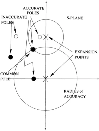
Another method for increa.sing AWE’s accuracy with multi point expansions is the Complex Frequency Hopping (CFH)[6]. Different from our method, the (JFH technique performs single expansions on several points cuid combines them into an accurate set of jioles and residues. This algorithm first performs single point expansions at s = 0 and s = jujmax , the lowest and highest frequencies of interest. The poles are coiriputed separately and a common pole is searched. If any pole is matched in both expansions, this pole is marked a.s accurate. Otherwise, another expansion point found using a. binary search algorithm[14]. The search continues until every two successive expansions have a.t least one common pole. The algorithm given below summarizes the technique and it is illustrated in Fig. 3.1.

• Step 1: Poles from each expansion point obtained as mentioned in [14]. • Step 2: Residues are computed as in the AWE technique [1].

Figure 3.1: Pole selection algoritlim in CFH

• Step 3: If the same poles are detected in two different expansions, they

are marked as accurate.

• Step 4 : The distance between an expansion point and its farthest accu­

rate pole defines the radius of accurcicy(/4cc)· All poles within this liacc are marked as accurate. •

• Step 5: Poles that are not marked and corresponding residues are said

to be inaccurate and rejected.

Chapter 4

M O M EN T G EN ER A TIO N

In previous chapter, we introduced two methods for multi point moment match­ ing. Now, we will introduce the evaluation of the moments for linear circuits. This chapter begins with matrix formulation of the circuit and it proceeds with computation of moments from that matrix.

4.1

Linear C ircuit Form ulation

Consider a linear network tt, which contains linear lumped components, and

arbitrary linear subnetworks. The subnetworks may contain distributed ele­ ments. The Modified Nodal Analysis (MNA) matrix equations of the network 7T can be written as:

Ns

W - z ( t ) + Hz(t) + ^ Dklk - huit) ( - U )

where

z(t) : node voltage vector appended by

independent voltage source current

and linear inductor current W matrix for energy storage

lumped components

H matrix for non energy storing lumped components

b vector for independent sources Dk selector matrix that maps ¿i·,

the currents entering subnetworks to node space

u{t) : input function

and for the subnetworks, we have

AkVfc + Bklk = 0 for A: = 1... (4.2)

Vk and Ik are terminal voltages and currents of the Â:th subnetwork. Writing the Laplace transform of the equations we obtain:

Dns

0

0 l2(s) = 0 i ‘{s) (4..3)

Bns

VVe call the MNA matrix T(s), vector of unknowns x(s), and the excitation vector w and form the circuit equation as (2.-5).

sW + H D i Ü2 A iD Î B i 0 A2D I 0 B2 ANs^ Ns 0 0 Z(s) b Ii(s) 0 l2(s) = 0 . In s(s) _ 0 16

4.2

E valuation o f M om en ts

As mentioned in chapter 3, the moments of circuits with both lumped and distributed components are computed according to Eq. 3.1. That is, we need to take the derivatives of the circuit matri.x: T in order to evaluate the moments. The first derivative of T at s = .sq is given as

'J'(l) —

w

0

0

0

A<y(so)DT

_Bi'’(so)

0

0

A^^^(so)Dj

0

B<^>(so)

0

(T4)

A

(

)D^^

0

0

_{BtJ>o) _}

0 T<r) _ A i^ (s o )D i A<’-)(so)D

0

0

0

'

'>(

)

0

0

0

Bi‘‘>(so)

0

0

0

Dir)

If the circuit has lumped components only, = 0 for r > 2. The Ak and Bk are the entries associated with transmission line moments. The moments of the transmission lines are found by using the eigenvalue moment methods or matrix exponential method. The details of the subject can be found in literature [2, 11, 3]. In our simulations we considered lossless transmission lines only. VVe will illustrate the evaluation of moments for lossless transmission lines in an example.

4.2.1

E xam p le

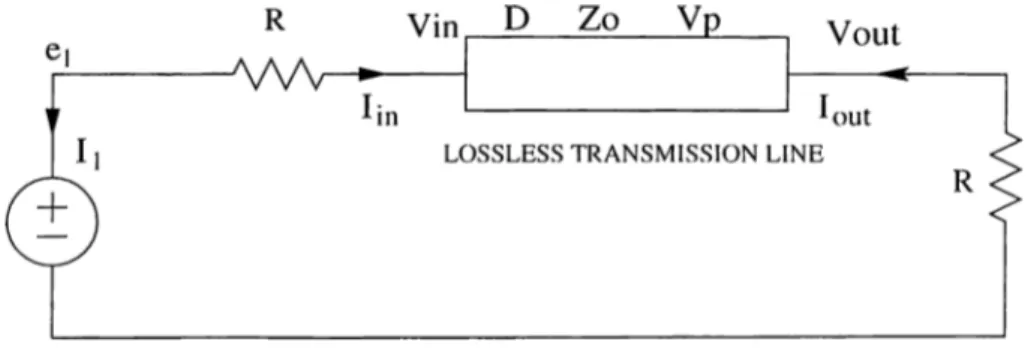
■Assume a lossless transmission line with the parameters D, Zq, Vp where D is the

length. Zq is the characteristic impedance and Vp is the phase velocity (Fig. 4.1).

These parameters can be calculated from the unit electriccil characteristics

{L,C) if the frequency and the type of the line is determined. The terminal

Figure 4.1: Illustrative example lor moment genercition voltages of the line are related by

Vinis) Voutis) + B louti^) = 0 where A = B Eii so) - E 2{so) / Zo 0 ZoEAso) 0 T’i(so) 1 and E i{ s ) = cosli(sD/vp) E 2 {s) = —sin h{sD/vp)

The derivatives at s = sq are obtained cis

E [ ' ' \so) 0 A(^) = B (’·) = Ei^'\so)IZo 0 ZoE!2''Hso) 0 e [''\.so) 0 18

where

E^ i s o ) = i

(^re

+(gre»p

^ Vv ' ^ I'v '

If we form the T matrix for this topology

l/Z^i - I / R y 0 1 0 0 l/i?i 0 0 1 0 0 0 _l/i?2 0 0 1 1 0 0 0 0 0 0 Ey - 1 0 ZqE-i 0 0 E2I Zq 0 0 Ex 1 ei v;„ h ^in lout

and the derivatives for r > 1 are

■ 0 0 'J'(r) _ 0 0 0 0 • 0 E f V Z o 0 0 0 0 0 0 1 0 0

Since there are no energy storage passive elements in the circuit, the W matrix in Ec[. 4.4 is set to zero. If we choose normalized values for the components

{R = 1, Zo = 0.5 and Djup = 1) we estimate the exact response as,

K)ui('S) — 0.5

cosh(s) + \..2osinh{s)

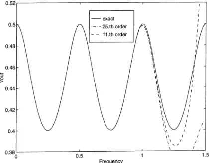
The response of AWE at 11th and 25th orders are depicted in Fig. 4.2 with the exact response. Since the exact response of such an circuit topology is periodic, it is impossible to approximate it by a rational. However, in most of the practical circuits, there are both energy storage elements and transmission lines and these circuits have dominant poles that enables us to approximate

their impulse responses with rationals. AWE methods are useful to cuialyze linear circuits when the dominant poles that are written in rationed powers of s, exemplifies the entire response.

Figure 4.2: Output of the one transmission line circuit

C hapter 5

C O M PU T A T IO N A L

C O N C E P T S

This section discusses the design of the siinulator in view of practical and nunierical concepts. First, we explain the properties of the siniula.tor a.nd pi'oceed with the nuinerical results.

5.1

A lgorith m o f th e sim ulator

The simulator we designed performs the following tasks in order; • Parsing the input file

• Forming the circuit matrix

• Calculation of frequency slufted moments a.ccording to the recui'sive scheme given in ( 3.1) and [2].

• Repetition of last step for each expansion point

• Matching moments to an aproxirnating rational and extracting the coef­ ficients

I

The input parser inputs files very similar to Spice input format [15]. The format of the input circuit file and the configuration file (.config) that deter­ mines the expansion points are explained in .\ppendix. The circuit matrix is determined by the information arranged by the input parser. Several sub­ routines are used to perform the analysis as expressed in options card. A commercial malri.x solver and the LlJ-solver implemented before are employed as external subroutines. The program produces a display output and an output file. The contents of the output is formated according to the options card as mentioned in Appendix.

5.1.1

S e le c tio n o f th e exp an sion p o in ts

Since we are employing a form of Fade Approximation and searching for ap­ proximating rational, only the dominant poles are crucial in our design. In time and frecjuency analyses, the poles closer to joj a.xis are important, therefore vve choose expansion points on juj axis. Once, we set our freciuency range of inter­ est, we can apply complex frequency hopping technique (CFH) as mentioned in chapter 3. The frequency range of interest is generally between DC and a maximum frequency (~ GHz in interconnect circuits ). The CFH technique gives the expansion points and the corresponding number of moments. VVe use this information in our method and obtain the Multi point Fade Approximation function.

5 .1 .2

E x tr a c tin g th e coefficients

In the first method the coefficients of the approximating function are obtained from a system of matrix equations(3.8). Each and nrik element has its complex conjugate row in matrix equations. Therefore this N x N complex m atrix system is equivalent to an x N real system of equations and can be solved using the ordinary elimination algorithms such as LU [13].

In the second method, we form the divided difference table according to the n ,’s and s,· s. The coefficients of the denominator are solved from the complex equations (3.12). This complex system is at x ^ order, and could be solved using a complex matrix solver. The coefficients of the nominator are obtained by only forward and backward substitutions (Eq. 3.11).

5.2

N u m erical issues

In our study, we are primarily interested in .-\C analysis and pole-zero extrac­ tion of interconnect circuits. Different from the conventional simulators, the program we propose solves the circuit matrix, only a few times. Since the LU factorization of the circuit matrix is known from the solution of the first moment vector, higher order moments are obtained by one forward and one backward substitution only. If the number of the expansion points is n -f 1, we have a total of n -)- 1 LU factorizations of the circuit matrix. Obtaining the moments of the circuit at DC + n points include n -|- 1 LU and FBS’s

where n,· is the number of moments at fth expansion point.

Our method is proposed to solve complex circuits and the orders of approx­ imations are generally large (~ 30-50) compared to the typical approximations employed by AWE technique(~ 4-12)[l, 2. 4]. Since the orders of matrix sizes and the orders of approximations are high in interconnect AC analysis, we need larger memory area, higher accuracy and consume more cpu time, compared to a typical AWE transient analysis problem. Because of the very large and very small numbers appearing in matrices, the method becomes ill-conditioned. The calculation of many moments (~ 10) at one expansion point results in very small numbers as successive moments, since each consecutive moment is smaller than the previous one by an order of ~ 10^ in typical networks. .Also, the powers of expansion points appearing in Eq. (3.6), yields very big numbers.

As the circuit expands, the ill-conditioned behavior of the matrix in Eq. 3.8 increases. The reason for that is the deviation between the first and the last moments obtained from an expansion point. We can overcome this problem by setting a limit value for the ratio of last and first moments of expansion point

Sk.

— ^kx _{i = 0, . . . , T i k ^ i}

For ckj smaller than a reasonable limit, the moments rui-, for i > j are not calculated. If j/’ is less than what CFH requires, further action is necessary. To preserve the same accuracy, the number of e.Kpansion points must be increased beyond what results from CFH technique.

-Also, frequency scaling should be applied to the energy storing elements in the circuit to increase accuracy as well as employing high precision arithmetic as explained in the next subsection.

5.2.1

U sin g high p recision a rith m e tic

The most obvious method to overcome accuracy problems is to use a higher precision arithmetic. Although we use double precision arithmetic in all op­ erations, we have accuracy problems in larger circuits, such as interconnects cascaded three times or more. A higher precision of arithmetic may be used instead of double precision, but then we have to consider the dramatically in­ creased CPU time. This work was done for AWE transient analysis in [14] and accurate results were obtained.

5 .2 .2

S ta b ility

Another observation about the method is the stability of approximated poles. Similar to the AWE technique. Multi point Fade Approximation technique may result in spurious right hand side poles as well. This is because of the nature of

Fade Approximations. The typical way to overcome this problem is to discard

unstable poles and solve for the remaining system of equations. However, in most of the unstable cases, the effect of the unstable pole is negligible in total approximation.

C hapter 6

E X A M PL E S

Severed examples are presented here to demonstrcite the periormance oi the methocl. Since our prirmiry concern is AC analysis, and this requires higher or­ ders of approximcitions than transient analysis, the circuits demonstrated here are at considerable sizes. In run-time estimations, a SUN-SPARC20 machine on UNIX is used and the averages of several run-times are considered. The accuracy of the clock used is 16 msec.

6.1

E xam p le 1

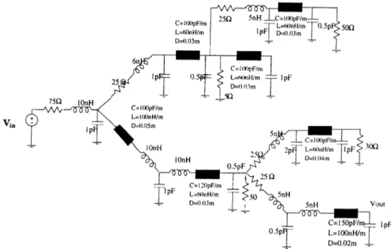
The first example is a well known interconnect circuit given in several relerences [8] [2]. As seen from Fig 6.1, the circuit has 29 lumped components, 7 lossless transmission lines and 21 nodes. Our frequency oi interest is 0 — 6G /7^. By applying CFH technique to this circuit, we found the order of approximation as 35. The expansion points and moment numbers are in Table 6.1. The AC response of the circuit computed according to the moment table. Scaling was taken as 1 x 10'^ for frequency dependent components.

The AC response Ii{s) of the circuit cuid the time comparisons are shown in IGg. 6.2 and lab le 6.2, respectively. As seen from the figure, the imdh point

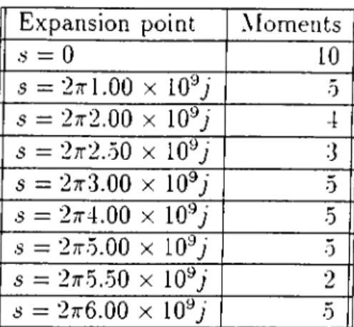
Figure 6.1: Example 1: Interconnect model with 7 transmission lines Expansion point Moments

s = 0 10

s = '2nl:2b X lO’^J 10

s = 27t2.50 X lO^j 10

■s = 27t.5.00 X 10^j 10

Table 6.1: Expansion points and the moment numbers for interconnect network in Ex. 1

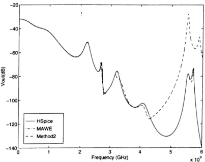
Fade approximation via Methodl (MAWE) and HSpice responses match each

other exactly, while Method2 has significant error at the end of frecpiency range. We can see from Table 6.2 that MAWE and Method2 spent much less time to get the same results as HSpice and Spice3. The high speed of Method2 resulted in loss of accuracy that makes it inefficient to use in AC analysis, while MAWE (Methodl) has a moderate time reduction without any loss of accuracy. When we calculate AC response at 6000 points in the frequency range 0 — 6GHz, the proposed MAWE computed nearly 11 times faster than HSpice and nearly 7 times faster than Spice3. In a 600 point .AC analysis, HSpice and Spice3 run times are closer to that of MAWE, but still MAWE has 3 or 4 times better

Figure 6.2; Output waveform for the interconnect network in Ex. 1 scores.

Simulator Real Analysis Time(sec)

6000 points 600 points MAVVE 1.1 0.9 METH0D2 0.6 O.o HSPICE 11.9 3.7 SPICE3 7.8 2.4

Table 6.2: Timing results for the interconnect network in Ex. 1 (I/O times excluded)

If we investigate the run time distribution diagram of the M.AWE intercon­ nect analysis (Fig. 6..3), we notice a remarkable time consumption for solving the coefficients according to Eq. -3.8. The slow behavior of the matrix solver used causes a speed disadvantage. The matrix system in (3.8) is large and nearly ill-conditioned in this example because of the high approximation or­ der. In order to solve this bad-mannered system, we employed a matrix solver in the available LAPACK library that resulted in loss of time. The LU process

shared insignificant time among all processes. This is due to the special LU solver implemented before by the Bilkent University C.\D group for solving the circuit matrix.

Interconnect circuit time disr.tjution

420

Figure 6.3: Run time distribution of MAWE for Example 1

6.2

E xam p le 2

Second example consists of two cascaded blocks, where the previous circuit is taken as a block (Fig. 6.4). Obviously, the circuit has twice more elements and nodes, i.e., 42 nodes, 14 lossless transmission lines and oS lumped components. We applied freciuency scaling as in the first example.

Figure 6.4: Example 2: Cascaded interconnects with 14 transmission lines ■Again, our frequency range is the same (0 — 6GHz). The expansion points and the number of moments for this circuit are given in Table 6.3. Since this

circuit is more complex and more stiff than the other one, we need to spread the expansion points to 8 points. The order of approximation increased as well, i.e., we now compute a total of 78 moments.

Expansion point s = 0 s = 27rl.00 X 10^; 5 = 2Tr2.00 X lO""; s = 27r2.oO X 10·^J s = 27t.3.00 X lO""; s = 2;r4.00 X •s = 2TT5.00 X 10^; s = 27t.5.50 X 10^7 Moments 10 s = 27t6.00 X lO^j

Table 6.3: Expansion points and the moment numbers for Example 2 The AC responses of cascaded interconnects computed by MAVVE and Methocl2 are compared with HSpice in Fig. 6.5. There is a slight difference between MAWE and Hspice (exact) responses, while Method2 has noticeable error. The slight error of M.AWE is acceptable since the absolute error never exceeds 3.5 x 10""* (Fig. 6.6).

The time comparison is given in Table 6.2. Method2 scored the best time again, but, the accuracy of Method2 is not sufficient enough to verify the AC analysis. MAVVE has still significant speed advantage over HSpice and Spice3. This time, the speed up over HSpice is 14 times and over Spice3 is 7 times in 6000 point analysis. We have similar results as examplel in 600 point analysis. M.AWE scored faster than both Spice simulators in this analysis as w'ell.

We were expecting MAWE to become faster as the circuit enlarges. How­ ever, as in this example, when the circuit size is doubled, the speed gain over Spice simulators do not have a noticeable change. After the investigation of the distribution in Fig. 6.7, we notice long time bars for solving coefficients ac­ cording to Eq. 3.8 and moment update according to Eq. 3.1. In this example, matrix solver consumed the longest time as well, because of the high approxi­ mation order and many expansion points used. .Again, this results in large and

Figure 6.5: AC Response of MAVVE in cascaded interconnect circuit in Ex. 2

Figure 6.6: Absolute error of MAWE response for Example 2

Simulator Real Analysis Time(sec) 6000 points 600 points MAWE 1.6 1.0 METHOD2 1.1 1.0 HSPICE 21.9 4.9 SPICE3 11.0 4.2

Table 6.4: Timing results for cascaded interconnects in E.x. 2 (I/O times ex­ cluded)

Cascaded interconnect circuit time distnbution

0 130

msec

Figure 6.7: Run time distribution of MAVVE for E.xample 2 ill-conditioned moment matrix systems that takes a long time to solve.

6.3

E xam p le 3

Our example is a lowpass filter with five transmission lines (Fig. 6.8) which was also investigated in [8]. The filter has 2 capacitors, 2 resistors and an inductor beside 5 lossless transmission lines. The expansion points and moment numbers for the filter is given in Table 6.5. The order of the approximation is 47, hence a total of 94 moments are calculated.

In Fig. 6.9, the output response of the lowpass filter is given. Methocl2 could not solve this ill-conditioned system. The responses of MAVVE and Hspice are indistinguishable. The frequency region of interest is 0 — 50GHz. The time comparisons between MAWE and Spice simulators and the run-time distribu­ tion of MAWE is given in Table 6.6 and Fig. 6.10, respectively. M.AWE reduced

Figure 6.8: Example 3: Lowpass filter with o transmission lines Expansion point Moments

5 = 0 10 s = 2irT2.5 X lO^i 10

s = 2TT25.0 X lO^i 10

s = 2x37.5 X 10*^/ 10

s = 2x50.0 X 10^/ 10

Table 6.5; Expansion points and moment numbers for the filter example analysis 4 times against Hspice and 3 times against Spice3 in 6000 point anal­ ysis. The speed recovery of MAWE against Spice simulators reduced in 600 point analysis.

The run-time distribution of MAWE in lowpass filter analysis is similar to the two preceding examples. Again, the matrix solver takes the longest time among all processes. Since there are 94 moments calculated, the matrix system in 3.8 has an order of 94 x 94. This takes 1000 msecs to solve the coefficients

Simulator Real Analysis Time(stc)

6000 points 600 points MAWE 1.9 1.4 HSPICE 7.5 3.4 SPICE3 5.2 1.4

Table 6.6: Timing results for the filter in Ex. 3 (1 /0 times excluded)

Figure 6.9: Lowpass filter output response

Time distribution for lowpass filter

1000

Figure 6.10: Distribution bars for the lovvpass filter analysis by MAWE in both 6000 and 600 point analyzes.

6.4

E xam p le 4

Ne.Kt. we will consider two rlc circuits in the same topology with 10 cells and 100 cells as given in Fig. 6.11. The circuits have 10 rlc elements with 21 nodes and 100 rlc elements with 201 nodes, respectively. The frequency range of interest in the first circuit is 0 — oGHz, while 0 — 2GHz in the second one. Scaling was applied to element values as 1 x 10^. The moment numbers and expansion

-a

AA/-L

--- WV-^—

Figure 6.11; Topology of the rlc circuits in E.\. 4 Expansion point s = 0 s = 2x2.50 X 10’^; ,s = 2x5.00 X lO""; Moments 12

Expansion point Moments .5 = 0 16

s = 2x1.00 X 10^;' 10 s = 2x2.00 X 10*^i 10

(a) (t·)

Table 6.7: Expansion points and moment numbers for (a) 21 and (b) 201 node rlc circuits

points are given in Table 6.7. It can be seen that, 28th order approximation is needed to find the response of 201 node circuit, while only 20th order is sufficient for 21 node circuit.

The output responses of two circuits are given in Fig. 6.12. VVe can see that, the exact response of HSpice is matched by M.AVVE for both circuits, while Method2 has significant loss of accuracy in both circuits. The time comparisons for both rlc circuits are given in Table 6.8. The time results of Method2 are excluded, since it has inaccurate responses compared to other simulators.

In RLC20, MAWE’s run time improvement against HSpice is in the order of 30, while in RLC200 the improvement is higher. This indicates that M.AVVE has better scores in a large analysis such contains 5000 points or more. This is valid for not only rlc circuits, but also interconnect circuits with distributed components.

(a) RLC20

Figure 6.12: AC Responses of the rlc circuits with 21 and 201 nodes

Simulator

Real Analysis Time (sec)

RLC20 RLC200

•5000 pts 500 pts •5000 pts •500pts MAWE 0.4 0.25 2.6 2.5 HSPICE 12.5 5.4 89 12.9 SPICE3 20.4 1.1 19 2.4

Table 6.8: Timing results for the rlc networks in E.x. 4 excluding I/O times

Time distnbution for RLC20 circuit

Time distnbutwn tor RLC200 circuit

f’igure 6.13: Run-tirne distributions of MAVVE for (a)RLC'20 (b)RLC200 in Ex. 4

When we look at time distributions of MAWE in Fig. 6.13, a major dif­ ference appears in two diagrams. The addition of the moment update process is dominant in 100 cell circuit (Fig 6.13a), while the addition of matrix solver dominates in 10 cell circuit (Fig 6.13b). In contrast to previous circuits and RLC20 circuit, the moment update takes longer time than the process of solv­ ing coefficients in RLC200 circuit. This is because of the large circuit matrix which is used in Eq. 3.1. This is due to the nearly 10 times larger circuit ma- tri.x compared to RLC20 circuit. This larger matrix which is used in recursive Eq. 3.1 causes many more multiplications than the multiplications needed for smaller size rlc network. Notice that, the data retrieving operations in moment update process consumes time as much as multiplication operations.

6.5

D iscu ssio n o f th e resu lts

The examples introduced before demonstrated the accuracy and efficiency of two methods. It is observed that MAWE (Multi point via Methodl) is faster than Spice like simulators in AC analysis of distributed networks especially in large analysis (more than 5000 points) without any significant loss of ac­ curacy. The reduction in time against HSpice is approximately on the order of 10 in large analysis, and 5 in small analysis. Although, Method2 is faster than MAWE and Spice simulators, it has quite large deviations from the exact response and failed to analyze circuits successively at this size. From this point of view, we propose MAWE to compete with conventional simulators.

Matrix Solver I/O PriKcss I/O Pnx;e.s.s LU Solver Moment Update Matn-x Solver ■ LU Solver Moment L'pdate (a) (b)

Figure 6.14: Time shares of all processes in a small and a large analysis VVe also observed that the recovery of MAVVE in analysis time obtained nearly without any accuracy loss. The responses of MAVVE and Spice simu­ lators are indistinguishable in the e.xamples e.xcept a few points and the error never exceeds acceptable limits.

When we look at the time distribution diagrams of MAWE, we notice two different situations occured. If the circuit is larger compared to the approx­ imation order, there appears a large circuit matrix, and the moment update process dominates in total time. The large circuit matrix involved in Eq. -3.1, is used in many multiplication and data retrieving operations. The sum of multi­ plications at one expansion point is 0{n] xn^). where Uc is the size of the circuit rnatri.x T and n; is the number of moments at that expansion point. Otherwise, higher approximation order compared to circuit size results in dominant time for matrix solver.

In the Fig. 6.14, the weights of all processes are given for a moderate MAWE analysis. The I/O process is the dominant time consumer in a large analysis. The moment update process and matrix solving process follows in order de­ pending on the situations mentioned above. In a small analysis, these two processes have more importance than I/O process as expected. Evaluation of points costs nearly as much as LU process in the large analysis, but, obviously LU becomes expensive in the small analysis. .Vs the circuits expand, the addi­ tion of LU on total time will increase; however, this will not cause dramatical changes in total execution time, since LU is performed once at each expansion point.

C hapter 7

C O N C L U SIO N

We have introduced a program with two methods for verifying the AC re­ sponse of linear circuits, using multi point moment matching techniques. Since Method2 gave inefficient results, iVIAWE (multi point Fade Approximation via M ethodl) is proposed to compete with Spice-like simulators.

Instead of calculating the frequency response at a large number of dis­ cretized points — like conventional simulators do — our program extracts the coefficients of an s-domain approximating rational of the impulse response. The proposed program can handle rlc circuits as well as the circuits with lossless transmission lines with no topological constraints, such as inductor loops, etc. The v’erification of the pole-zero analysis can also be done by the proposed pro­ gram. The execution time of MAWE compared to Spice-like simulators is 8-10 times better. This improvement can be rnultipled by using a better matrix solver. The performance of the simulator increases as the matrix solver’s ex­ ecution time decreases. Hence, MAWE will have a better run-tirne advantage against Spice-like simulators by means of an LU solver faster than the one we used.

The effectiveness of the program for large sized circuits can be extended by increasing the number of expansion points and distributing the required number of moments to these points.

This program can also handle multi-conductor transmission line circuits by using an approach presented in [2]. Finally, our simulator can perform tfc^nsient analysis of larger networks easily because of the nature of transient analysis which recjuires lower order of approximation (4-8). The recovery of the execution time in transient analysis will be similar to AC analysis as well.

A P P E N D IX A

I /O FO RM AT OF THE

P R O G R A M

A .l

C onfiguration F ile (.config)

The example .config file that defines the expansion points and corresponding moment numbers is given. The order of approximation is 46 and for example the number of moments at .s = 0 + j3.0 x 10'^ is 8.

46 0 0 14 0 1.5e9 10 0 3.0e9 8 0 4.5e9 12 0 6.0e9 9 40

A .2

C ircuit Input F ile (in lin .sp )

****** Exajnple interconnect network resl 1 2 75 lindl 2 3 lOe-9 capO 3 0 le-12 res2 3 4 25 lind2 4 5 6e-9 capl 5 0 le-12 trll 5 0 6 0 C=100e-12 L=60e-9 D= . 03 cap2 6 0 .5e-12 res3 6 0 50 res4 6 7 25 lind3 7 8 5e-9 cap3 8 0 le-12 vin 1 0 1

.ac le7 6e9 le7

.options useawe scaling=le9 lapack .print v(8)

. end

Transmission line : nodel node2 node3 node4 C=vaIue(F) L=value(//) D=length(m) Resistor

Capacitor Inductor Voltage Input

: r.K.x.x nodel node2 vaIue(Ω) : cx.xx nodel node2 value (F) ; Ixxx nodel node2 value [H)

: vxxx nodel node2 value (V )

A .2.1

O p tions Card

.options :

printmb : Prints T and T'" at each moment computation showiterno : Prints iteration number

useawe : Employs AWE and multi point subroutines to verify the analysis poles : Prints poles and residues of the circuit

lapack : Employs commercial Lapack package rnatri.x solver instead of another solver implemented before

methocl2 : Employs Methocl2 to verify the analysis moments : Prints moments at each e.xpansion point post ; Prints every step to output file

scaling : Inputs scaling value i,e, scaling= le9 list : Prints every step to display

A .2.2

O ther C ards

.print : Defines output parameter to be printed, i.e, print v(node number)

• tran : Determines the transient analysis, i.e, tran time-step stoptime

.ac : Determines the ac (frequency) analysis, i.e., ac startfreq stopfreq stepfreq

.clc : Determines the dc analysis, i.e., dc startvolt stopvolt stepvolt

A .3

O u tp u t o f th e program

The output of the program for the input and .config files above b given next. The output consists of an output file and display output. The output file stores the number of discrete frequencies and the corresponding voltages in absolute values in a neat format which could be easily loaded by graphics tools (Matlab, Mathematica,...). The display output is as follows:

data file is interconnect/Awefiles/inl.out scaling

-This is the

beginning-Parsing Time=0 sec.

MNA matrix forming time for (0,0)=0 sec. LU time=0 sec.

First FBS time=0 sec.

Other moments (13) evaluation time=0.016666 sec. MNA matrix forming time for (0,1.5)=0 sec.

LU time=0 sec.

First FBS time=0 sec.

Other moments (9) evaluation time=0 sec.

MNA matrix forming time for (0,3)=0.016666 sec. LU time=0 sec.

First FBS time=0 sec.

Other moments (7) evaluation time=0 sec. MNA matrix forming time for (0,4.5)=0 sec. LU time=0 sec.

First FBS time=0 sec.

Other moments (11) evaluation ti me=0.016666 sec. MNA matrix forming time for (0,6)=0 sec.

LU time=0 sec.

First FBS time=0 sec.

Other moments (8) evaluation time=0 sec.

Lapack matrix solving time =0.799968 sec. ♦***rcond = 3.1096e-59 numerator of order 45 (0.333333,0) (-0.148894,-0.133465) (0.0813455,0.0139253) (-0.00395075,0.00700985) (-0.000353988,-0.000384566) .... (-3.93383e-40,7.23369e-41) (1.71645e-41,6.20467e-42) denominator of order 46 (1,0) (-0.0821817,-0.400394) (0.140346,-0.104168) (0.056108,0.0125836) (0.00711239,0.00681182) (0.00147754,0.00166321) .... (-1.50432e-37,1.54943e-37) (-4.3418e-39,2.25196e-39) (-2.74136e-40,3.49853e-40)

Evaluation time for given frequency range =0.116662 sec.

Evaluation time without io =0.033332 sec.

Total time=l.23328 sec. --- That' s the end—

R E F E R E N C E S

[1] L T. Pillage, and R. A. Rohrer. Asymptotic waveform evaluation for timing analysis. IEEE Transactions on Computer Aided Design^ 9:352- 366, April 1990.

[2] Так К. Tang, and Michel S. Nakhla. .Analysis of high-speed vlsi intercon­ nects using the asymptotic waveform evaluation technique. IEEE Trans­

actions on Computer Aided Design of Integrated Circuits and Systems,

ll(3):341-352. March 1992.

[3] J.E. Bracken, V. Raghavan, and R. A. Rohrer. Interconnect simulation with asymptotic waveform evaluation. IEEE Transactions on Circuits and

Systems-I: Fundernantal Theory and Applications, 39:869-878, Nov 1992.

[4] X. Huang, V. Ragvahan, and R. k . Rohrer. Awesim: .A program for the efficient analysis of linear(ized) circuits. In Tech. Dig., pages 534-537. ICCAD, Nov. 90.

[5] D. F. Anastakis, N. Gopal, S.Y. Kim, and L.T. Pillage. On the stability of approximations in asymptotic waveform evaluation. In Proc. Design

Automation Conference, May 1993.

[6] Michel S. Nakhla and Eli Chiprout. .Analysis of interconnect networks using complex frequency hopping (cffi). IEEE Transactions on Computer

Aided Design of Integrated Circuits and Systems. 14(2): 186-200, February

1995.

[7] Peter Feldmann and Roland W. Freund. Efficient linear circuit analysis by pade approximation via the lanczos process. IEEE Transactions on

Computer Aided Design of Integrated Circuits and Systems, 14(5):639-

649, May 1995.

[81 Mustafa Çelik, Oğan Ocali, Mehmet A. Tan, and Abdullah Atalar. Pole- zero computation in microwave circuits using multi point pade approx­ imation. IEEE Transactions on Circuits and Systems-1: Eundarnental

I

Theory and Applications^ 42(I):6-13. .January 1995.

[9] Chi-Tsong Chen. Linear System Theory and Design. Holt-.Saunders In­ ternational Editions, 1984.

[10] .Jiri Vlach and Kishore Singhal. Computer methods for circuit analysis

and design. Van Nostrand Reinhold Company. 1983.

[11] Eli ChiproLit and Michel S. Nakhla. .\ddrfissirig high-speed interconnect issues in asymptotic waveform evaluation. In Design Automation Confer­

ence., 1993.

[12] .\nnie Cuyt and Luc VVuytack. Nonlinear Methods in Numerical Analysis. North-Holland, 1988.

[13] S. D. Conte and C. De Boor. Elementary numerical Analysis. Mc- GrawHill, Singapore, 1981.

[14] Eli Chiprout and Michel S. Nakhla. Asymptotic Waveform Evaluation

And Moment Matching for Interconnect Analy.sis. Kluwer Academic Pub­

lishers, 199- .

[15] Meta-Software. Hspice User’s Manual, 1992.