^ İ - Î ■; ÿ } · / ·;·,·./«5 . '<«✓ -л. V j¿jL - * * - C '^JT* «ώ.-f"- --.^ гі"··- ./*V. ' · ?"Гі‘ ;·“': .i-, - , ,^·\
W
г іГ"
·<^
і51 i г
i
:
J
.
:
^
■Гѵ .■■■■* í i i i ■·? '.^ ·'' Ş ··-.. · '. .■/ · V. /· ’ 7 · ,· ./ ‘"J i:nc^ í 7 ^-. -K, .«. 5 - ‘« « r¿,529,s
• k S T fBS¿i)PERFORMANCE MEASUREMENT OF PORTFOLIOS CONSTRUCTED BY THE SINGLE INDEX MODEL WITH HISTORICAL AND ADJUSTED BETAS
A THESIS
SUBMITTED TO THE FACULTY OF MANAGEMENT
AND THE GRADUATE SCHOOL OF BUSINESS ADMINISTRATION OF BILKENT UNIVERSITY
IN PARTIAL FULFILLMENT OF THE REQUIREMENTS FOR THE DEGREE OF
MASTER OF BUSINESS ADMINISTRATION
by
H G -ц ^5L£>.Ç
- h г Я
I 3 ï > 4
В022е?3
I certify that I have read this thesis and in my opinion it is fully adequate, in scope and quality, as a thesis for the degree of Master of Business Administration.
Assoc. Prof. Kursat Aydogan
I certify that I have read this thesis and in my opinion it is fully adequate, in scope and quality, as a thesis for the
I certify that I have read this thesis and in my opinion it is fully adequate, in scope and quality, as a thesis for the degree of Master of Business Administration.
Assist Prolf. Gulnur Muradoglu
Approved for the Graduate School of Business Administration
Prof. Dr. Subidey Togan
J /
A B S T R A C T
This study investigates the performance of portfolios
constructed by single index model with historical (least
squares regression) betas and estimated future betas by
Vasicek's Bayesian Estimation Technique. The performances of the portfolios are measured by Sharpe's reward to variability ratio. The portfolios constructed by the simple criteria for portfolio selection of Elton, Gruber, Padberg have outperformed the market, but not at a statistically significant level. This is caused by the low market volume and high volatility of the market. The correlation between the market and the stocks turned out to be very low. Also the betas of the stocks were
very volatile. Previous studies have shown that Vasicek's
adjusted beta outperforms the historical one, but in this study, this could not be shown for the Istanbul Stock Exchange.
Keywords: Single index model, historical beta, bayesian
0g ^ I s of future betas, adjusted beta, reward to
Bu çalışma tekil indeks modeli yardımıyla geçmiş beta ve
gelecekteki tahmini beta kullanılarak oluşturulmuş
portföylerin performanslarını ölçmek amacıyla yapılmıştır.
Portföylerin performansları Sharpe'ın getiri değişkenlik
oranına göre ölçülmüştür. Elton, Gruber, Padberg’in
yöntemiyle oluşturulan portföyler piyasadan daha iyi
performans göstermişler, fakat bu sonuç istatistiksel
belirginlikte olmamıştır. Bunun sebebi, piyasanın derinliğinin
az olması ve değişkenliğinin yüksek olması olarak
gösterilebilir. Piyasa ve hisse senetlerinin korelasyonları
düşük olarak bulunmuştur. Aynı zamanda hisse senetlerinin
betaları dönemden döneme çok değişkenlik göstermektedir. Daha önceki çalışmalar Vasicek^in betasının geçmiş betaya göre daha
iyi performans gösterdiğini belirtmekle beraber, aynı olgu
İMKB için bu çalışmada gösterilememiştir.
Anahtar Kelimeler: Tekil indeks modeli, geçmiş beta,
bayesian gelecek beta tahmini, düzeltilmiş beta, getiri
değişkenlik oranı.
Ö Z E T
I have received much help and contribution from many individuals in preparing this study. I am very grateful to the Bilkent University Management Department and especially to the Associate Professor Kursat Aydogan because of the support he has provided, while supervising me. I would also like to thank
to my otlier thesis committee members Assc. Prof. Gökhan
Capoglu and Asst. Prof. Gulnur Muradoglu for their valuable comments and suggestions which contributed a lot to the product.
I also thank the Capital Market Commission for providing me the data essential for this study. I am also grateful to Interbank, especially Mr. N. Kavuşturan, for supporting me.
In addition, I would also like to thank my colleagues for their comments and supports.
ACKNOWLEDGEMENTS
ABSTRACT... i
OZET... i i ACKNOWLEDGEMENTS... İİİ I) INTRODUCTION... 1
II) LITERATURE REVIEW... 4
III) DATA AND METHODOLOGY... 13
3.a) Estimation of Historical Betas and Future Betas...15
3.b) Construction of Portfolios with the Single Index Model... 16
3.c) Comparison of the Performance of the Market, Historical and Adjusted Beta Portfolios...19
IV) ANALYSIS OF THE DATA... 21
V) SUMMARY AND CONCLUSIONS... 28
VI) REFERENCES... 31
APPENDIX 1) LIST OF STOCKS CONSIDERED FOR PORTFOLIO CONSTRUCTION... 35
APPENDIX 2) STATISTICAL T-TEST RESULTS...37
APPENDIX 3) THE VARIANCE OF BETAS OF INDIVIDUAL STOCKS... 39
APPENDIX 4) THE VARIANCE OF BETAS IN THE PERIODS... 43
APPENDIX 5) THE COMPOSITION OF PORTFOLIOS...44
APPENDIX 6) HISTORICAL BETAS OF ALL STOCKS BY PERIODS... 47
APPENDIX 7) ADJUSTED BETAS OF ALL STOCKS BY PERIODS... 53
APPENDIX 8) HISTORICAL BETAS DURING THE PERIOD 1989-1990.... 59
APPENDIX 9) ADJUSTED BETAS DURING THE PERIOD 1989-1990... 61
APPENDIX 10) HISTORICAL PORTFOLIO OF 1989-1990...63
APPENDIX 1 1) ADJUSTED PORTFOLIO OF 1989-1990...64
APPENDIX 12) RISK FREE RATES (6-MONTH T-BILL RATES)... 65 TABLE OF CONTENTS
LIST OF TABLES
Table 1: Number of Stocks Included in the Study in
Each Period... 13
Table 2: Average Values of Stocks... 21
Table 3: Betas of Some Key Industries... 22
Table 4: Stocks with Negative Betas... 22
Table 5: Five Highest Beta Stocks and Their Betas... 23
Table 6: Four Stocks with Betas Close to One... 23
Table 7: Reward to Variability Ratios of Portfolios... 24
Table 8: Fieward to Variability Ratios of Portfolios of 1989-1 990 in 1991... 26
Tcible 9: Stocks that Appear in the Portfolios More Than Once... 27
I ) INTRODUCTION
The Capital Asset Pricing Model of Treynor [19], Sharpe [17], and Lintner [16] states that the expected rate of return on a security in excess of the risk-free rate is proportional to the slope coefficient of the regression of that security's rates of return on a market portfolio. The slope coefficient, or beta, is for this reason one of the basic concepts of modern capital market theory, and considerable attention has )30ei-i devoted to its measurement.
Customarily, beta is estimated from past data by
least-squares regression procedures. The least squares
technique consists of fitting a linear relationship between the rates of return on a security and the rates of return on a market index so that the sum of squared differences between
the security's actual returns and those implied by the
relationship is minimized.
An essential prerequisite for using beta to assess future
portfolio risk and return is a reasonable degree of
predictability over future periods. If the portfolio manager cannot predict future beta coefficients, the applicability of
this phase of modern capital market theory is somewhat
restricted. Blume [5], Vasicek [20], Merill Lynch, Pierce, Fenner, & Smith Inc. proposed different techniques to predict future betas.
The objective of this thesis is to test the effectiveness of one of the prediction techniques, namely Vasicek's bayesian estimation of security betas, compared to historical betas by practically using these betas in portfolio selection. The set of stocks that will be considered for the portfolios are the stocks traded at the Istanbul Stock Exchange. The portfolio selection criteria used is the one proposed by Elton, Gruber, Padberg [9][10 ] .
If it can be shown that the adjusted beta portfolios perform better than historical beta portfolios, the results of this thesis can be used by portfolio managers who want to invest in the Istanbul Stock Exchange to construct optimal portfolios of the future which will beat the market as well as
the historical beta portfolios. Sharpe's [18] reward to
variability ratio is utilized to measure the performances of the portfolios.
However, it could not be shown that the historical and
adjusted portfolios beat the market portfolio at a
statistically significant level, although these portfolios
outperformed the market portfolio.
In section II, previous studies in the literature will be reviewed. In section III, data and methodology used in the study will be discussed. In section IV, the data will be analyzed and findings will be presented. In section V, summary
of the study and comments will be provided and areas for future studies will be given.
The concept of beta of a stock is one of the basic concepts of modern capital market theory, and considerable attention has been devoted to its measurement.
O.A. Vasicek [20] presented a method for generating
Bayesian estimates of the regression coefficient of rates of
return of a security against those of a market index. He used
the distribution of the regression coefficients across
securities as the prior distribution in the analysis and gave
explicit formulas for the estimates. He concluded that
Bayesian estimates are preferred to the classical sampling theory estimates for the following reasons: First Bayesian procedures provide estimates that minimize the loss due to
misestimation, while sampling theory estimates minimize the
error of sampling. This is because Bayesian theory deals with
the distribution of the parameters given the available
information, while sampling theory deals with the properties of sample statistics given the true value of the parameters. Secondly, Bayesian theory weights the expected losses by a
prior distribution of the parameters, thus incorporating
knowledge which is available in addition to the sample
information. This is particularly important in the case of estimating betas of stocks, where the prior information is usually sizable.
II) LITERATURE REVIEW
beta coefficients, at least in the context of a portfolio of a large number of securities, were relatively stationary over
time. Nonetheless, there was a consistent tendency for a
portfolio with either an extremely high or low estimated beta in one period to have a less extreme beta estimated in the
next period. In other words, estimated betas exhibited a
tendency to regress towards the grand mean of all betas, namely one.
Blume [3] used a cross sectional regression of security betas computed for two adjacent periods as the basis for
adjusting his predictions of beta for the subsequent,
nonoverlapping period. The adjusting equation was a simple linear regression of beta for security j in period 2, /3 ., on
2 j
the corresponding coefficient for period 1, /3^q
/ 3 = 6 + 5 6 +C.
' 2j 0 1 ij j
where 6 and 8 are least squares regression coefficients and
0 1
e is a random disturbance term. J
Merill Lynch, Pierce, Fennei, & Smith Inc. (MLPFS) makes
use of an adjustment procedure which, like Blume's indicator, is based on a cross sectional regression of historical betas for consecutive nonoverlapping time periods. Beta estimates
are adjusted toward a mean of one using the following
p = 1.0 + k ( 1 . 0 )
' 2j 1 J
where B is the estimated beta coefficient of security j in
ij
period 1, k is a constant common to all stocks, and B . is the
2 j
adjusted beta used to predict the /3 in the second period.
Levy [15] found that single security beta coefficients of one period were not good predictors of the corresponding betas in the subsequent period. However, as portfolio size was increased, the stationarity of extrapolated betas improved significantly. A major problem for both single security and portfolio betas was the tendency for relatively high and low
beta coefficients to over predict and under predict,
respectively, the corresponding betas for the subsequent time period. Thus, forecasting accuracy grew progressively worse as beta levels departed significantly from the average.
Black, Jensen, Scholes [2], Blume, Friend [4], and Fama,
MacBeth [12] explained this regression tendency in the
following way: For some unstated economic or behavioral
reasons, the underlying betas do tend to regress towards the mean over time. Yet, even if the true betas were constant over time, it has been argued that the portfolio betas as estimated in the grouping period would as a statistical artifact tend to be more extreme than those estimated in a subsequent period. This bias has been termed an order or selection bias.
Marshall Blume [5] showed that estimated beta coefficients tend to regress towards the grand mean of all betas over time and he presented two kinds of empirical analyses which showed that part of this observed regression tendency represented real nonstationarities in the betas of individual securities and that the so called order bias was not of overwhelming importance. In other words, companies of extreme risk (either high or low) tend to have less extreme
risk characteristics over time. There are two logical
explanations. First, the risk of existing projects may tend to
become less extreme over time. This explanation may be
plausible for high risk firms, but it would not seem
applicable to low risk firms. Second, new projects taken on by firms may tend to have less extreme risk characteristics than existing projects. If this second explanation is correct, it is interesting to speculate on the reasons. For instance, is it a management decision or do limitations on the availability of profitable projects of extreme risk tend to cause the riskiness of firms to regress towards the grand mean over time? But Blume did not determine the explicit reasons behind this phenomenon.
R.C. Klemkosky and J.D. Martin [14] investigated the sources of forecast errors of extrapolated beta coefficients and three adaptive procedures recommended by Vasicek, Blume, and Merill Lynch, Pierce, Fenner, & Smith Inc. for improving beta forecasts. Klemkosky and Martin [14] found that all three
unadjusted forecasts as denoted by the reduction in mean square error and the inefficiency component. In one period
MLPFS adjustment technique was most successful, followed
closely by Blume's technique and lastly by the Bayesian adjustment. However, in two consecutive periods, the Bayesian adjustment achieved the greatest reduction in total mean
square erroi . They concluded that the accuracy of the simple
no-change extrapolative beta forecast can be improved. A
combination of the Bayesian predictor and a reasonable
portfolio size would make beta coefficient a highly
predictable risk surrogate.
In 1 973 Elton and Gruber [8] published an article in
which they investigated the accuracy of forecasts of the correlation structure between securities produced by a group of alternative models. As pointed out in that article, while analysts may be capable of providing estimates of returns and
variances, the development of estimates of correlation
coefficient from anything other than models utilizing
historical data is highly unlikely. The article, after
investigating the accuracy of certain forecasting techniques,
suggested that those techniques which provided the best
forecasts could lead to a simplification of the portfolio problem.
Fisher Kamin [13] found that the naive forecast of beta as one performed surprisingly well compared to some more
sophisticated techniques
Elton, Gruber, and Urich [11] re-examined the forecasting ability of some of the techniques which provided the best set
of forecasts in Elton Gruber [8] as well as some new
variations of these techniques. The techniques compared in Elton, Gruber, and Urich [11] are:
1) Full historical correlation model: The simplest method of estimating future correlation coefficients using historical data is to assume that past values of these coefficients are the best estimates of their future values.
2) Single index models
a) Unadjusted betas: These are the betas obtained from a least square regression of security returns on a market index during some historical period.
b) Vasicek adjustment to betas. c) Blume's beta adjustment.
d) Beta of one for all stocks: This estimate is obtained by assuming that all betas are one.
3) Constant correlation model: This assumes that
historical data only contains information concerning the mean correlation coefficients and that observed pairwise differences from the average are random, so
that zero is a better estimate of their future value.
The most aggregate averaging possible is to
set every correlation coefficient equal to the average of all correlation coefficients.
Elton, Gruber, Uriah [11] demonstrated that constant correlation model is a preferred method of forecasting future correlation coefficient in comparison to the best of the Beta time series techniques. The Vasicek beta adjustment technique ranked the second best technique. In addition they discussed the bias, in the mean estimate produced by standard beta estimating techniques. Correcting for this bias had no effect on the dominance of constant correlation model but did change the ranking within the beta techniques.
In their article Bos and Newbold [6] discussed the
market model in which the possibility is allowed that beta is stochastic and obeys a first order auto regressive process. They estimated and tested such models on a large sample of monthly returns of common stock. They found strong evidence indicating stochastic systematic risk, but relatively little evidence against the random coefficient model.
Collins, Ledolter, Rayburn [7] employed a model that
allows beta to exhibit both random and auto regressive behavior simultaneously to investigate whether the variation in beta is purely random or exhibits auto correlation through time. They tested the model against alternative specifications on a large sample of individual securities and randomly formed portfolios comprising 10, 50, and 100 securities. They found that it was difficult to detect statistically the sequential varicition in the betas of individual securities, while there might exist such a variation. They also found that aggregating
individual securities into portfolios tends to strengthen the auto regressive tendencies of beta.
Berglund, Liljeblom, Loflund [1] examined the properties
of different market risk (beta) measures computed on daily data for a thin security market like the Helsinki Stock Exchange in Finland. The paper showed differences in trading frequency between different stocks produced a serious bias towards what appeared to be stability in estimated betas. Furthermore the paper showed that when betas are computed, the exclusive use of stock prices based on actual trades would not solve the problem of a thin trading bias in measured stability of these beta estimates. The results indicate that none of the corrections as such are likely to produce much improvement compared to ordinary least squares betas. In fact it turned out that the mean of the betas for the previous period is almost as accurate as a predictor for the future betas as are the individual betas.
Winston, T.L., and Yueh, H.C. [21] examined three
important issues concerning the pricing of securities and the
investment horizon, namely, the length of the investment
horizon, the sensitivity of the beta coefficient to the
assumed horizon, and the correlation between the beta and the horizon estimates. Their major findings are: 1) A capital
asset is risky because it has a nonzero beta and the
investment horizon is finite. 2) The beta estimate is
generally quite sensitive to the assumed horizon; the smaller
the horizon, the more sensitive beta is to the change in horizon. 3) The betci and horizon estimates are correlated either negatively or positively.
The raw data is the weekly closing prices of the stocks
traded in the Istanbul Stock Exchange and the closing
composite market index. The data is collected for the years between 1988-1991. The data in the 1986-1988 period has been excluded from the study, as the stock market was very thin and open to speculation in that period.
The number of stocks in six month periods considered for portfolio construction in the market is as follows:
Table 1 : Number of stocks included in the study in each
period
Ill) DATA AND METHODOLOGY
Period 1988-1 1988-2 1989-1 1989-2 1990-1 1990-2 1991-1
Number 44 46 46 49 49 87 1 07
The stocks considered for portfolio construction are those which are actively traded from the beginning of the period till the end of the period. Stocks that are rarely traded during the period are discarded. This elimination has been done to ensure statistical reliability of the data. The list of stocks considered for portfolio construction is given in Appendix 1.
The raw data is not suitable for return computations, as there are high downfalls due to stock splits, dividends and
capital increases. Therefore the raw data has to be adjusted for these events.
First, daily closing prices of the stocks in the Istanbul Stock Exchange are adjusted according to dividends and capital increases. The prices before the increase or dividend are multiplied with the following ratio.
R =
0P-D+I*1000 1 +I + S
OP Where
OP: Price before the day of increase or dividend. D
I S
Cash dividend in T.L. Capital increase ratio. Split Ratio.
Risk free rates are required for the sake of portfolio construction for each period. The risk free rate used in this
study is the 6-month T-bill rate set by the Department of
Treasury in the auctions. The period of 6 months is chosen to
match the investment horizon of the portfolio and the risk free rate. This is essential to eliniinate interest rate risk. The T-bill rates used in this study are given in Appendix 12.
From these adjusted daily closing prices, weekly returns are calculated for all the stocks and the ISE composite index. These weekly returns are afterwards grouped in periods of six months. Then for each period of six months, returns of all the stocks are regressed with respect to the market index returns (where the independent variable: return of the market, and the
dependent variable: return of the stock). This regression
2 2
process provides us the /3ji, of the stocks where:
ji
III.a) Estimation of Historical Betas and Future Betas:
/3ji : /3 of the stock i in period j.
cr^ : Variance of error in Y estimate of stock i in period j . ji
cr^ : Variance of error in /3 estimate of stock i in period j. pji
With the historical /3 of the stock a new f3 estimate is
made according to the bayesian estimation technique of
O.A.Vasicek [20]. An estimate for the next period is
Ccilculated with the following formula.
O' /32İ = /31 i ^/3ii ^ ^/3i /3i + 2 /3ii where
/3ii : /3 of the stock i in period 1 .
cr^ : Variance of error in /3 estimate of stock i in period 1 .
pi i
/3i : Average of betas of all stocks in period 1 .
2
: Variance of betas of all stocks in period 1.
At the end we obtain two betas for every stock in each
period. These betas will be utilized in the process of
constructing portfolios.
Ill.b) Construction of Portfolios with the Single Index Model:
Given the /3's, average returns of individual stocks
optimal portfolios can be constructed with the simple criteria
for optimal portfolio selection proposed by E.J.Elton,
M.J.Gruber, M.W.Padberg [9],[10].
Assumptions of the Single index model:
1) The returns of individual stocks (or portfolios) are related to the market return in a linear relationship where the relationship is:
R = R + ( R - R ) / 3
i f m f i
The algorithm proposed by Elton, Gruber, Padberg
assumes that all pairwise correlation coefficients are equal. 2) There exists a risk-free rate asset in the market.
3) There exists an investment alternative whose expected return is greater than the risk-free asset.
4) Investors try to maximize the reward-to-variability of their investments.
These assumptions and the simple criteria algorithm give
us the tangent point of the efficient frontier and the
risk-free rate.
The algorithm for this construction procedure is as follows:
Group the stocks into two; One group consisting of
negative /3, the other non-negative ¡3 stocks. Rank the positive /3 stocks with respect to their volatilities, where volatility is defined as: V = i R - R i f Volatility of stock i 13.
R. : Average return of stock i. R : Risk free rate.
f
: /3 of stock i.
Among the positive volatility stocks, starting with the highest, compute the following ratio:
<p = a m k
I
i = l R - R i f C i k R^
^
m1
— 2^ i=1 cr C iO' : Variance of market returns.
m
2
cr : Variance of error of Y estimate
c i
This computation is done for each stock till V - <f>
k ^k
becomes negative. Positive - (p^ stocks are included in the
portfolio.
After positive /3 stocks are finished, stocks with
negative /3's should be tried. From these stocks the ones with
positive volatilities are discarded. Starting with the
smallest volatility, must be computed until no more
stocks enter. If any negative stocks enter, it must decrease
the size of the term in brackets in 0^ and so the highest
excess return to positive /3 stocks previously rejected should be checked to see if it now enters. If more positive /3 stocks enter, then the negative /3 stock list should be checked and the procedure repeated iteratively until no more stocks enter. In actual practice this iterative procedure will converge almost instantaneously because of the very small number of stocks with negative ¡B's.
For each stock entering the portfolio, Z.is computed to find the ratio of that stock in the portfolio.
Z = i C i R - R i f - <t>.
From Z.'s the normalized stock ratios ( ) can be found
a s :
K y Z.
III.c) Comparison of the Performance of Market, Historical and Adjusted Beta Portfolios
Given the algorithm above optimal portfolios are
constructed for each half of each year between 1 988 - 1991.
The weekly returns of the portfolios constructed in one period
(one with historical and the other with adjusted /3's) are
computed for the consecutive period. For example the portfolio constructed in the first half of 1988, is held long in the second half of 1988 and its weekly returns are computed. Given these returns, average and variance of returns are calculated.
For each period of six months W.F.Sharpe's [18] reward to
variability ratios of every portfolio and the market index are computed.
Sharpe's reward to variability ratio is
R = p
R - R
p f
R : Average return of the portfolio.
p
cr^ : Variance of returns on portfolio. p
Then the reward to variability ratios of historical, adjusted and the market portfolios are statistically tested whether their means are equal with t-test procedure.
Beside these tests, two portfolios have been constructed from the stocks in the period 1989 - 1990 and the performance of these portfolios have been measured in the year 1991. All
the methods and algorithms apply to this measurement as well.
IV) ANALYSIS OF THE DATA
Previous studies Marshall Blume [3,5], Fisher, Kamin [13] have shown that the grand mean of betas of stocks in a period approac[ies one. However in ISE this is not the case. In most of the periods investigated, the averages of betas of stocks in the market are less than one. Only in two periods they are close to one. In the second half of 1990, the beta average is
0.35 which is a very surprising result. This could be
explained by the way we are taking the average of the betas of stocks. The average is the simple arithmetic mean, and this mean does not take the trading volume of individual stocks into consideration. Whereas the market index is computed weighted by the trading volume of stocks comprising the index.
Therefore in a thin market such as ISE, the returns of
individual stocks and the market index are not much correlated
(see Table 2). The values of stocks are very low as it can
be seen in the table.
Table 2: Average values of stocks
1988-1 1988-2 1989-1 1989-2 1990-1 1990-2 1991-1
0.385083 0.321729 0.345528 0.402965 0.519258 0.173167 0.401425
When the average of betas of industries over seven periods are computed, the highest beta industry turns out to
be the cement industry, where the lowest beta industry is tourism (Table 3).
Table 3: Betas of some key industries
INDUSTRY AVG BETA
CEMENT 1 .228019 METAL 0.760649 HOLDING 0.717336 TEXTILE 0.627218 BANKING 0.383243 TOURISM 0.268053
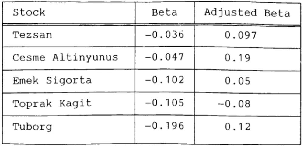
There are five stocks which have negative beta average over seven periods. Their names and betas are given in Table
4. These stocks have low volume, offered to the public
recently. Also the length of the period causes the betas to be negative, because in short periods stocks may have negative correlation with the market, but in the longer term they take positive betas.
Table 4: Stocks w^ith Negative Betas
Stock Beta Adjusted Beta
Tezsan -0.036 0.097
Cesme Altinyunus -0.047 0.19
Emek Sigorta -0 . 1 0 2 0.05
Toprak Kagit -0.105 -0.08
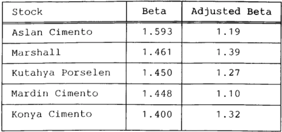
A small sample of stocks which have very high average betas, and another sample of stocks which have betas close to one fire listed in Tables 5 and 6 respectively with their average betas. Historical and adjusted betas of all stocks are listed in Appendices 6 and 7.
Table 5: Five Highest Beta Stocks and Their Betas
Stock Beta Adjusted Beta
Aslan Cimento 1 . 593 1.19
Marshall 1 . 461 1 . 39
Kutatıya Porselen 1 . 450 1 . 27
Mardin Cimento 1 . 448 1.10
Konya Cimento 1 . 400 1 .32
Table 6: Four Stocks with Betas Close to One
Stock Beta Adjusted Beta
Sarkuysan 1.012 0.98
Doktas 0.996 0.95
T .Demirdokum 0.993 0.97
Erdemir 0.992 0.93
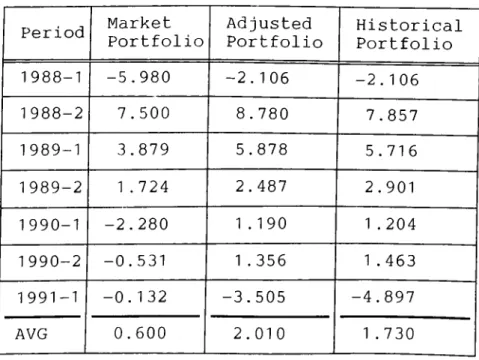
After the reward to variability ratios had been computed, they were compared with each other. The averages of reward to variability ratios of the portfolios constructed by Elton,
Gruber, Padberg's [9],[10] algorithm with historical and adjusted betas were greater than the reward to variability of
the market portfolio, but this result was not at a
statistically significant level (See Table 7 for the reward to variability ratios, and Appendix 2 for statistical tests). The
reason for that was the size of the sample (only seven
periods), and the high variance of the reward to variability ratios which is caused by high volatility of the market.
Table 7: Reward to Variability Ratios of Portfolios
Period Market Portfolio Adjusted Portfolio Historical Portfolio 1988-1 1988-2 -5.980 7.500 -2.106 8.780 -2.106 7.857 1989-1 3.879 5.878 5.716 1989-2 1 . 724 2.487 2.901 1990-1 -2.280 1.190 1 . 204 1990-2 -0.531 1 . 356 1 . 463 1991-1 AVG -0.132 0.600 -3.505
2.010
-4.897 1 .730The averages of the reward to variability ratios of adjusted and historical beta portfolios are very close to each other and they are statistically not different. This implies
that Vasicek's adjustment procedure did not improve the
performance of portfolios of ISE stocks at a statistically significant level. Previous studies (R.C. Klemkosky and J.D.
Martin [14], Elton, Gruber, Urich [11]) have shown the significant superiority of Vasicek's beta over historical beta in the U.S. market. The reason why the result of this thesis which is not in line with previous studies, can be explained by the length of the periods where betas are computed. In this thesis this period is six months while in previous studies this period is five years. In six months the slope coefficient of the linear regression is very much variable as it can be seen in Appendix 3.
Also the variance of betas of stocks (see Appendix 4)
v/ithin one period is very high, which makes Vasicek's
adjustment not a useful tool, because it heavily depends on the variance of betas within a period. When this variance is high the adjusting formula returns a beta close to the historical one which makes the adjustment not very useful. This is also a very important reason why the adjusted beta portfolios could not significantly beat the historical beta portfolios.
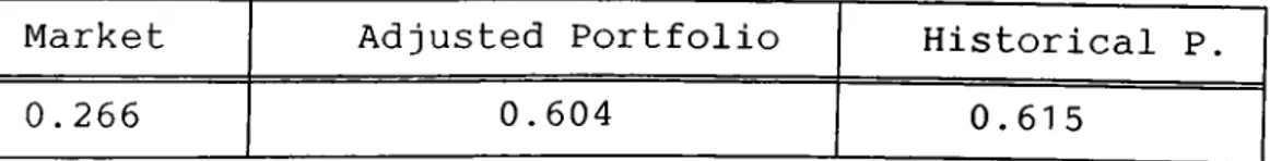
The second part of the analysis in which two portfolios are constructed by the weekly returns of stocks and the market index in the period 1989-1990 and the performances of these portfolios and the market index are measured in the year 1991, gives us the same result as the first part. Both portfolios perform better than the market but the adjusted portfolio performs worse than the historical portfolio. The historical
and the adjusted betas are provided in the Appendices 8 and
9 respectively. The composition of the portfolios are given
in Appendices 10 11 , The reward to variability ratios are
provided in Table 8.
Table 8: Reward to variability ratios of portfolios of
1989-1990 in 1991
Market Adjusted Portfolio Historical P.
0.266 0.604 0.615
When the composition of portfolios are considered for a
given period, the adjusted and historical beta portfolios
comprise mostly the same stocks with close percentages. This is the case because adjusted betas and historical betas are
close to each other for the reason mentioned above. See
Appendix 5 for the composition of portfolios.
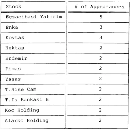
Eczacibasi Yatirim stock has appeared in the portfolios five times out of seven portfolios. This makes Eczacibasi Yatirim the first in order of appearance. The stocks which appear more than once in the portfolios are given in Table 9 with their number of appearances.
Table 9: Stocks that Appear in the Portfolios More Than Once Stock Ц- of Appearances Eczacibasi Yatirim 5 Enka 3 Koytas 3 Hektas 2 Erdeinir 2 Pimas 2 Yasas 2 T.Sise Ccim 2 T.Is Bankasi В 2 Кос Holding 2 Alarko Holding 2
21
V) SUMMARY AND CONCLUSIONS
In this thesis, the performances of the Istanbul Stock Exchange market portfolio and portfolios constructed with historical and adjusted betas were examined. The portfolios are constructed according to the single index model using the algorithm proposed by Elton, Gruber, Padberg [9][10]. The
performance measure utilized was Sharpe's [18] reward to
variability ratio.
After the reward variability ratios had been computed, they were compared with each other. The averages of reward to variability ratios of the portfolios constructed by Elton,
Gruber, Padberg's [9],[10] algorithm with historical and
adjusted betas were greater than the reward to variability of
the market portfolio, but this result was not at a
statistically significant level. The reason for that was the size of the sample (only seven periods), and the high variance of the reward to variability ratios which is caused by high volatility of the market.
The averages of the reward to variability ratios of adjusted and historical beta stocks are very close to each other and they are statistically the same. This implies that Vasicek's adjustment procedure did not improve the performance of portfolios of ISE stocks at a statistically significant
level. Previous studies (R.C. Klemkosky and J.D. Martin [14],
Elton, Gruber, Uriah [11]) have shown the significant
superiority of Vasicek's beta over historical beta in the U.S. market. The result of this thesis which is not in line with previous studies, can be explained by the length of the periods where betas are computed. In this thesis this period is six months while in previous studies this period is five years.
Also the variance of betas of stocks within one period is very high which makes Vasicek's adjustment not a useful tool, because it heavily depends on the variance of betas within a period. When this variance is high the adjusting formula returns a beta close to the historical one which makes the adjustment not very useful. This is also a very important
reason why the adjusted beta portfolios could not
significantly beat the historical beta portfolios.
When the composition of portfolios are considered for a
given period, the adjusted and historical beta portfolios
comprise mostly the same stocks with close percentages. This is the case because adjusted betas and historical betas are close to each other for the reason mentioned above.
Previous studies Marshall Blume [3], [5], Fisher Karnin
[13] have shown that the grand mean of betas of stocks in a period approaches one. However in ISE this is not the case. In most of the periods investigated, the averages of betas of
stocks in the meirket are less than one. This could be explained by the way we take the average of the betas of stocks. The average is the simple arithmetic mean, and this mean does not take the trading volume of individual stocks into consideration. Whereas the market index is computed weighted by the trading volume of stocks comprising the index.
Therefore in a thin market such as ISE, the returns of
individual stocks and the market index are not much
correlated.
In the light of the characteristics of the Istanbul Stock
Exchange, portfolio managers cannot beat the market
significantly with the help of the portfolio selection
criteria and beta adjustment technique that we have used. The practicality of these techniques should be checked in the future when the market gains depth and stability.
1. Berglund, T., Liljeblom, E., and Loflund, A., "Estimating Betas on Daily Data for a Small Stock
Market," Journal of Banking and Finance, vol. 13,
1989, pp. 41-64.
2. Black, F., Jensen, M.C., and Scholes, M . , "The Capital
Asset Pricing Model: Some Empirical Tests," in
Michael Jensen, ed.. Studies in the Theory of
Capital Markets. New York: Praeger Publishing, 1972.
3. Blume, M. "On the Assessment of Risk," Journal of
Finance, March 1971.
4. Blume, M. and Friend, I. "A New Look at the Capital
Asset Pricing Model," Journal of Finance, March
1973.
5. Blume, M.E., "Betas and Their Regression Tendencies,"
Journal of Finance, Vol. 30, No. 3, June 1975,
pp. 785-795.
6. Bos,T. and Newbold, P., "An empirical Investigation
of the Possibility of Stochastic Systematic risk in the Market Model," Journal of Business, 1984, vol. 57, No 1, pp. 35-41.
VI) REFERENCES
7 . Collins, D.W., Ledolter, J. , and Rayburn, J. , "Some Further Evidence on the Stochastic Properties of Systematic Risk, Journal of* Su s x u g s sf 1987, vol. 60, no. 3, pp.425-448.
8. Elton, E.J. and Gruber, M.J., "Estimating the
Dependence Structure of Share Prices," Journal of
Finance (December, 1973) pp. 1203-1232.
9. Elton, E.J., Gruber, M.J., and Padberg, M.W., "Simple Criteria for Optimal Portfolio Selection," Journal
of Finance, Vol. 31, No. 5, December 1 976,
pp.1341-1357.
10. Elton, E.J., Gruber, M.J., and Padberg, M.W., "Simple Criteria for Optimal Portfolio Selection: Tracing Out the Efficient Frontier," Journal of Finance, Vol. 33, No. 1, March 1978, p p . 296-302.
11. Elton, E.J., Gruber, M.J., and Urich, T.J., "Are Betas Best?" Journal of Finance, vol. 33, no. 5, 1978, pp. 1375-1384.
12. Fama, E.F., and MacBeth, J.D., "Risk Return and
Equilibrium: Empirical Tests," Journal of Political
13. Fisher, L. and Kamin, J., "Good Betas and Bad Betas,"
Paper for the Seminar on the Analysis of Security Prices, University of Chicago, November, 1971.
14. Klemkosky, R.C. and Martin, J.D., "The Adjustment of Beta Forecasts," Journal of Finance, Vol. 30, No. 4, September, 1975, pp. 1123-1128.
15. Levy, R.A., "On the Short-Term Stationarity of Beta
Coefficients," Financial Analysts Journal, 27
(November-December 1971), pp. 55-62.
16. Lintner, J., "The Valuation of Risk Assets and the Selection of Risky Investments in Stock Portfolios
and Capital Budgets," Reviev of Economics and
Statistics, February 1965.
17. Sharpe, W.F., "Capital Asset Prices: A Theory of
Market Equilibrium Under Conditions of Risk,"
Journal of Finance, September 1964.
18. Sharpe, W.F., "Mutual Fund Performance," Journal of
Business, Vol. 39, Pait 2, January 1966, pp. 119-138.
19. Treynor, J.L., "Toward A Theory of Market Value of Risky Assets," unpublished memorandum, 1961.
20. Vasicek, O.A., "A Note On Using Cross-Sectional
Information In Bayesian Estimation Of Security
Betas," Journal of Finance, Vol. 28, December 1973,
pp. 1233-1239.
21. Winston, T.L., and Yueh, H.C., "Investment Horizon
and Beta Coefficients," Journal of Business
Appendix 1) List of stocks that are considered for portfolio construction ARAL t e k s t i l AKBANK AKSA ALARKO HOLDING ANADOLU CAM(ACS) ARCELIK ASELSAN ASLAN CIMENTO AYGAZ BAGFAS BOLU CIMENTO BRISA ÇANAKKALE CIMENTO ÇELİK H CESME ALTINYUNUS CIMSA ÇUKUROVA DEMIRBANK d e n i z l i DEVA HOLD DOGUSAN DOKTAS ECZ ILAC ECZ YAT EGE END EGEB EGEG EMEK SIG ENK ERCIYASB ERE FENIS ALIMINYUM GOOD-YEAR GORBON ISIL GÜBRE FABRİKALARI GÜNEY BİRACILIK HEKTAS I. MOTOR p i s t o n i k t i s a t f i n.k i r INTEMA IZMIR d e m i r ç e l i k IZOCAM KARTONSAN KAV KELEBEK m o b i l y a KENT GIDA KEPEZ ELEKTIRIK КОС h o l d i n g КОС YATIRIM KONYA ç i m e n t o KORDSA KORUMA TARIM KOYTAS KÜTAHYA PORSELEN MAKINA TAKIM MARDİN ç i m e n t o MARET MARMARİS MARTI MARSHALL MENSUCAT SANTRAL METAS NASAS NET BANK NET t u r i z m 35
FINANSBANK NETHOLD.
GENTAS OKAN TEKS
OLMUKSA YUNSA
OTOSAN YAPI k r e d i
PARSAN YASAS
PEG PROFILO UŞAK s e r a m i k
PETKIM v e s t e l PIMAS PINAR ET PINAR SU PINAR SUT PINAR UN POLYLEN RABAK SABAH YAY SANTRALHOLD. SARKUYSAN SI FAS SOKSA T. HAVA YOLLARI T.d e m i r d o k u m T.DISBANK T.g a r a n t i b a n k T.IS BANKASI(B) T.SIMENS T.s i s e c a m T .TUBORG TAM SIG t e k s t i l b a n k TELETAS TEZSAN TOPRAK KAĞIT TRAKYA CAM TSKB TUNCA TEKSTİL TUTUNBANK
Appendix 2) Statistical t-test results
ROW MARKET ADJ HIST
1 -5.9800 -2.1060 -2.1060 2 7.5000 8.7800 7.8569 3 3.8789 5.8781 5.7159 4 1.7240 2.4866 2.9014 5 -2.2800 1.1900 1.2044 6 -0.5310 1.3556 1.4632 7 -0.1318 -3.5046 -4.8969 MTB > twos cl c2
TWOSAMPLE T FOR MARKET VS ADJ
N MEAN STDEV MARKET 7 0.60 4.34 ADJ 7 2.01 4.27 SE MEAN
1
.6
1
.6
95 PCT Cl FOR MU MARKET - MU ADJ: (-6.5, 3.7)
TTEST MU MARKET = MU ADJ (VS NE): T= -0.61 P=0.55 DF= 11
MTB > twos cl c3
TWOSAMPLE T FOR MARKET VS HIST
N MEAN STDEV SE MEAN
MARKET 7 0.60 4.34 1 .6
HIST 7 1 . 73 4.35 1 .6
95 PCT Cl FOR MU MARKET - MU HIST: (-6.3, 4.0)
TTEST MU MARKET = MU HIST (VS N E ): T= -0.49 P=0.63 DF= 11
MTB > twos c2 c3
TWOSAMPLE T FOR ADJ VS HIST
N MEAN STDEV SE MEAN
ADJ 7 2.01 4.27 1 . 6
HIST 7 1 . 73 4.35 1 .6
95 PCT Cl FOR MU ADJ - MU HIST: (-4.8, 5.4)
TTEST MU ADJ - MU HIST (VS NE): T= 0.12 P=0.91 DF= 11
MTB > aovone c1-c3 ANALYSIS OF VARIANCE SOURCE DF SS MS F P FACTOR 2 7.9 3.9 0.21 0.812 ERROR 18 336.3 18.7 TOTAL 20 344.1
INDIVIDUAL 95 PCT Cl'S FOR MEAN BASED ON POOLED STDEV
LEVEL N MEAN STDEV — +--- +--- --- +- --- +—
MARKET 7 0.597 4.340 (---*--- --- ) ADJ 7 2.011 4.272 (--- --- ) HIST 7 1 . 734 4.355 (--- --- ) POOLED MTB > STDEV = 4.322 -2.5 0.0 2.5 5.0
A p p e n d ix 3) The variance of betas of individual stocks STOCK VAR INTEMA 0.925348 ALARKO HOLDING 0.396066 GENTAS 0.367955 GOOD-YEAR 0.359826 TSKB 0.332438 NET BANK 0.330443 MAKINA TAKIM 0.327256 YAPI k r e d i 0.315805 MENSUCAT SANTRAL 0.313822 PIMAS 0.300538 MARET 0.299053 KAV 0.298446 IZMIR d e m i r ç e l i k 0.255676 METAS 0.248964 EGE GÜBRE 0.246613 MARDİN ç i m e n t o 0.241816 GÜNEY BİRACILIK 0.232408 EGE END 0.229974 ECZ YAT 0.228857 NASAS 0.222326 CIMSA 0.212999 TAM s i g o r t a 0.210475 OLMUKSA 0.203688 ENKA 0.200362 OKAN t e k s t i l 0.199816 MARMARİS MARTI 0.199416 PINAR SUT 0.1887 GORBON ISIL 0.185583 d e n i z l i 0.183256 GÜBRE FABRİKALARI 0.181053 BRISA 0.174511 POLYLEN 0.172186 39
STOCK VAR EGE b i r a AKAL t e k s t i l DEVA HOLD ERDEMIR KORUMA TARIM YASAS ANADOLU CAM(ACS) ERCIYAS b i r a 0.169472 0.168902 0.167164 0.163396 0.162697 0.158334 0.157769 0.155933 ÇANAKKALE CIMENTO 0.151875 SIFAS IZOCAM KORDSA T.d e m i r d o k u m ECZ ILAC AKSA SARKUYSAN PINAR UN HEKTAS i k t i s a t f i n.k i r BAGFAS T.IS BANKASI(B) BOLU CIMENTO YUNSA SOKSA T.SIEMENS ç e l i k h a l a t PINAR SU KOYTAS DOGUSAN RABAK КОС YATIRIM PINAR ET TELETAS DEMIRBANK VESTEL 0.148819 0.142485 0.138764 0.130436 0.121544 0.118721 0.117915 0.116969 0.115698 0.112289 0.109738 0.109356 0.104259 0.102351 0.09774 0.097455 0.093781 0.085707 0.085125 0.084653 0.084168 0.079906 0.079036 0.076179 0.075497 0.075279
STOCK VAR T.g a r a n t i b a n k FINANSBANK SANTRALHOLD. KARTONSAN SABAH YAY ÇUKUROVA ARCELIK OTOSAN DOKTAS KEPEZ ELEKTIRIK T.s i s e c a m EMEK s i g o r t a PEG PROFILO T.TUBORG КОС HOLDING AYGAZ t e k s t i l b a n k PETKIM KELEBEK m o b i l y a CESME ALTINYUNUS NETHOLDING KENT GIDA TOPRAK KAĞIT TRAKYA CAM TUNCA t e k s t i l FENIS ALIMINYUM I. MOTOR p i s t o n AKBANK TUTUNBANK UŞAK s e r a m i k T.DISBANK NET t u r i z m T. HAVA YOLLARI ASLAN ç i m e n t o PARSAN 0.075162 0.068716 0.06773 0.0677 0.066317 0.064706 0.06468 0.063758 0.06025 0.056574 0.055497 0.046393 0.044502 0.042497 0.036722 0.022963 0.01824 0.006261 0.000807 0.000344 2.8E-06 0 0 0 0 0 0 0 0 0 0 0
0
0 0 41STOCK VAR KONYA CIMENTO TEZSAN ASELSAN MARSHALL KÜTAHYA PORSELEN
0
0
0
0 0Appendix 4) Variances of l>etas in the periods 1988-1 1988-2 1989-1 1989-2 1990-1 1990-2 VAR 0.244399 0.155135 0.313975 0.127959 0.079888 0.076287 1991-1 VAR 0.226804 4 3
Appendi;< 5) The composition of portfolios
Adjusted 1988-1 Historical 1988-1
Stock Percent Stock Percent
CIMSA 100.00% CIMSA 100.00%
Adjusted 1988-2 Historical 1988-2
Stock Percent Stock Percent
ENKA 36.70% EGE BIRA 15.92%
MENSUCAT 17.04% MENSUCAT 18.66%
EGEB 8.83% ENKA 33.07%
GUNEY BIRA 15.67% HEKTAS 10.66%
HEKTAS 7.60% GUNEY BIR 11 .07%
ERDEMIR 12.35% ERDEMIR 10.62%
OTOSAN 1.81%
Adjusted 1989-1 Historical 1989-1
Stock Percent Stock Percent
MARINA TA 8.14% PIMAS 6.10%
YASAS 14.85% KAV 17.43%
KAV 13.48% YASAS 17.30%
EGEB 3.50% KARTONSAN 19.56%
KARTONSAN 17.95% NASAS 4.99%
PIMAS 2.85% ECZ YAT 15.54%
ERE 18.49% ERE 13.37%
NASAS 2.63% SIFA& 2.69%
ECZ YAT 14.06% T.SISE CA 3.03%
Adjusted 1 Stock____ TSKB YAPI KRED MARET KOYTAS T.IS BANK PIMAS КОС YATIR КОС HOLDI YASAS ECZ YAT ARCELIK HEKTAS 989-2 _Percent 6.30% 16.73% 18.57% 8.89% 6.64% 3.74% 8.67% 7 7 4 7 , 50% 40% 64% 55% 3.37! Adjusted 1990-1 Stock_____ ALARKO HO 21 .43% ECZ YAT 26.25% KOYTAS 16.05% ENK 9.98% KOC HOLDI 9.34% DEVA HOLD 10.20% MAKINA TA 3.80% KEPEZ ELE 2.95% Adjusted 1990-2 Stock_____ ECZ YAT 29.58% MARDİN c i m 3.16% ECZ ILAC 27.00% AYGAZ 15.84% T.I& BANK 12.17% ALARKO HO 2.38% AKSA 3.56% T.s i s e c a m 6.32% Historical 1989-2 Stock Percent PIMAS 9.44% YAPI KRED 17.97% KOYTAS 8.85% MARET 18.30% BOLU c i m e 3.45% T.IS BANK 6.89% КОС YATIR 7.82% YASAS 6.85% КОС HOLDI 6.15% ECZ YAT 4.16% HEKTAS 4.35% ARCELIK 5.78% Historical 1990-1 Stock Percent ALARKO НО 24.79% ECZ YAT 26.30% KOYTAS 12.92% MAKINA TA 10.63% ENK 7.50% КОС HOLDI 1 1 . 26% DEVA HOLD 5.80% BAGFAS 0.80% Historical 1990-2 Stock Percent ECZ YAT 31.07% ALARKO HO 4.54% ECZ ILAC 27.09% MARDİN c i m 2.44% T.IS BANK 11.77% AYGAZ 13.75% AKSA 4.82% T.SİSE CAM 4.52% 45
Adjusted 1991-1 Historical 1991-1
Stock Percent Stock Percent
TUNCA ТЕК 65.43% NETHOLD. 7.03%
SVKSA 7.68% TUNCA ТЕК 67.03%
DOKTAS 15.37% SVKSA 7.51%
ECZ YAT 6.18% DOKTAS 14.16%
NETHOLD. 1 . 94% ECZ YAT 1 . 70%
ENKA 2.26% ENK 1 . 20%
Appendix 6) Historical betas of all stocks by periods 1988-1 1988-2 1989-1 1989-2 ALARKO HOLDING GOOD-YEAR TSKB MARINA TARIM YAPI RREDI MENSUCAT SANTRAL PIMAS MARET RAV
IZMIR DEMİR CELIR METAS EGE GUBRE GUNEY BIRACILIR ECZ YAT NASAS CIMSA OLMURSA ENRA PINAR SUT d e n i z l i GUBRE FABRIRALARI BRISA POLYLEN EGE BIRA ERDEMIR RORUMA TARIM YASAS ANADOLU CAM(ACS) SIFAS IZOCAM RORDSA T.d e m i r d o r u m 1 .1 51966 1.400038 -0.14283 -0.08753 0.064021 0.354876 -0.21116 0.205475 1.608233 0.436411 1 0.234796 0.48392 0.22818 1.270665 1.905185 -0.01091 -0.07544 0.210188 1.03274 0.228849 0.785542 0.781227 0.402237 0.152669 1.512509 0.614576 1.234281 1.150673 0.811654 0.949463 0.603348 0.378853 0.50061 1.207304 0.401327 0.567156 1.881453 1.394532 0.803477 0.518322 0.589646 0.789556 0.316152 0.007448 0.875932 0.984834 0.261057 0.862588 0.687013 1.153349 1.164614 1.298885 1.546587 1 . 586796 1.634299 -0.16194 -0.04462 0.16592 -0.38521 0.8171 0.046208 0.027446 0.317295 0.097818 0.819377 0.326333 1.007649 0.602181 0.430742 1.633196 1.042465 1.451002 1.349789 0.802726 0.759702 0.390148 0.304157 1 .677957 0.826386 0.612862 0.851349 0.135293 0.756793 0.664375 1.052873 -0.03113 0.286691 0.574398 1.213704 1.032307 0.384133 1.232588 -0.0917 0.594092 1.846448 1.211605 1.68664 0.578111 0.257168 0.684813 0.759471 0.399571 0.803959 0.864686 0.718055 1.45146 0.580085 0.99108 1 47
I 9 8 8 - I
I 9 8; 8 2
I 9 89-1
1989-2 SARKUYSAN HEKTAS BAGFAS T.IS BANKASI(B) BOLU ç i m e n t o T.SIEMENS ç e l i k h a l a t KOYTAS RABAK КОС YATIRIM TELETAS KARTONSAN ÇUKUROVA ARCELIK OTOSAN DOKTAS KEPEZ e l e k t i rIК T.s i s e c a m КОС h o l d i n go .896515
0 . 7 32 6 67
1 . 591 335
0 . 4 0 5 5 4 6
1 . 2 01 0 53
0 .5 5 97 7 5
0 . 9 1 1 1 4 3
0 . 3 1 8 2 8 4
0 . 8 2 4 7 6 4
0 .7 6 21 9 2
0 . 5 57 28 î
1 .2 9 76 16
0 . 9 2 1 1 0 3
0 . 9 1 9 7 0 6
1 .1 6 86 25
0 . 6 8 5 5 0 2
0.604531
0 . 9 0 1 8 1 8
I . 0 5 8 3 5 9 I 0.414848
0.697276 0.219624 0.92002 0.42674 0.863004 0.202789 0.737783 0.4 9 0 I () 9 0.4 4 809 3 0.452729 0.8 3 28,0 3 0.87 5 6961
. 2 0 1 1
58
0.89 08 5 2 0.4 9 2 21 4 0.6 5 2 4 20 . 8 4 7 8 2 2
17 495 1.116356 1.414661 0.633189 0.782455 0.94296 1.265952 0.107903 1 . 29 258 0.5 3 127 0. 166994 0 . 481 168 1 . 18,2 158 0.9 11 65 3 0.707472 0.81767 0.949937 1 . 1 1 9 032 0.9 59684 0.912667 0.639541 0.906521 0.595253 0.167029 1.176005 0.820788 0.47646 1.282453 0.692271 0.856949 0.736176 1.166623 0.840907 0.89842 1.24582 0.782657 0.855506 0.7970131990-1 1990-2 1991-1 INTEMA ALARKO HOLDING GENTAS GOOD-YEAR TSKB NET BANK MAKINA TAKIM YAPI k r e d i MENSUCAT SANTRAL PIMAS MARET KAV IZMIR d e m i r ç e l i k METAS EGE GÜBRE MARDİN ç i m e n t o GÜNEY BİRACILIK EGE END ECZ YAT NASAS CIMSA TAM s i g o r t a OLMUKSA ENKA OKAN t e k s t i l MARMARİS MARTI PINAR SUT GORBON ISIL d e n i z l i GÜBRE FABRİKALARI BRISA POLYLEN EGE b i r a AKAL t e k s t i l 0.341807 1.213567 1.379917 0.642881 1.509155 1.020614 1.805388 1.097449 1.564291 0.992885 1.306651 0.988695 0.569997 1.494424 1.374792 0.97224 1.077558 1.094685 1.288635 1.410339 0.170657 0.036992 0.263328 -0.1377 0.30633 0.028029 1.082763 0.118068 0.134818 0.41106
1
0.116744 0.034759 0.098479 0.141262 0.956684 0.150018 0.274866 0.216168 0.129961 0.414669 0.231879 0.466346 0.243886 0.332133 -0.0839 0.380232 0.030501 0.201011 0.157255 0.190646 0.956907 0.405499 0.293961 2.094558 1.284536 1.476514 0.485249 0.834739 1 .17771 2 1.250571 0.743733 1.337008 1.477304 1.380485 1.435717 1.249477 1 .717148 1.095706 1 .9401 79 1.023466 1.233978 1.797013 1.114373 1.379189 1.149429 1.022706 1.226627 1.226148 0.809218 1.250271 0.892089 1.189882 1.300946 1.063367 1.052823 1.039508 1.115914 491990-1 1990-2 1991-1 DEVA HOLD 1 .167621 ERDEMIR 0.740125 KORUMA TARIM 1.190973 YASAS 1.28677 ANADOLU CAM(ACS) 0.796799 ERCIYAS b i r a ÇANAKKALE CIMENTO SIPAS 1.456242 IZOCAM 1.039508 KORDSA 1.221294 T.d e m i r d o k u m 1.416732 ECZ ILAC AKSA SARKUYSAN 0.898838 PINAR UN HEKTAS 1.210823 i k t i s a t f i n.k i r BAGFAS 0.923337 T.IS BANKASI(B) 0.970496 BOLU CIMENTO 0.907334 YUNSA SOKSA T.SIEMENS 1.052169 ç e l i k h a l a t 0.768428 PINAR SU KOYTAS 0.971242 DOGUSAN RABAK 1.388175 КОС YATIRIM 1.011572 PINAR ET TELETAS 0.821085 DEMIRBANK VESTEL T.g a r a n t i b a n k 0.269344 1.101969 0.497916 0.989488 0.803915 1.242292 0.589997 1.044661 0.141621 0.848888 0.175118 0.964884 0.42393 1.203351 0.559105 1.400191 0.19327 1.433243 0.296195 0.963693 0.239286 1.190275 0.459713 1.156975 0.236038 0.925156 0.407468 1.335842 0.114919 0.798933 0.245414 1.045491 0.137649 0.807839 0.637986 1.156852 0.452927 1.262935 0.77551 1.199037 0.360541 1.000388 0.312082 0.93735 0.560248 1.273436 0.351625 1.343662 0.362474 0.947989 0.590744 0.800122 0.241892 0.823795 0.581018 1.017199 1.227022 1.208877 0.258217 0.820485 0.588863 1.181399 0.038979 0.588514 0.617445 1.166184 0.273203 0.821519
1990-1 1990-2 1991-1 FINANSBANK SANTRALHOLD. KARTONSAN SABAH YAY ÇUKUROVA ARCELIK OTOSAN DOKTAS KEPEZ ELEKTIRIK T.SISE CAM EMEK s i g o r t a PEG PROFILO T.TUBORG КОС HOLDING AYGAZ t e k s t i l b a n k PETKIM KELEBEK m o b i l y a CESME ALTINYUNUS NETHOLDING KENT GIDA TOPRAK KAĞIT TRAKYA CAM TUNCA t e k s t i l FENIS ALIMINYUM I. MOTOR p i s t o n AKBANK TUTUNBANK UŞAK s e r a m i k T.DISBANK NET TURİZM T. HAVA YOLLARI 0.081496 0.60577 0.595554 1.116053 0.837401 0.169246 1.019856 0.491645 -0.0234 0.9659 0.624539 0.850387 0.595101 0.509653 1.360394 1.187293 0.582765 1.31525 1.188561 0.517628 1.1401 1.300977 1 0.923743 1.23286 0.585358 0.815527 0.114789 -0.31599 1.075812 1.497723 0.010586 -0.40171 0.895286 0.440372 1.11398 0.679746 0.982816 0.187535 -0.08258 0.271942 0.430193 0.406147 0.462973 -0.06592 -0.02884 0.211716 0.21506 0.201058 -0.10492 0.738014 0.440637 0.064203 0.419022 0.105583 0.005605 0.831024 0.371847 0.041493 0.715439 51
1990-1 1990-2 1991-1 ASLAN ç i m e n t o 1.593368 PARSAN 1.015599 KONYA ç i m e n t o 1.401594 TEZSAN -0.03683 ASELSAN 1.085898 MARSHALL 1.461026 KÜTAHYA PORSELEN 1.449711
Appendix 7) Adjusted betas of all stocks by periods 1988-1 1988-2 1989-1 1989-2 ALARKO HOLDING ANADOLU CAM(ACS) ARCELIK BAGFAS BOLU ç i m e n t o BRISA CELIK H CIMSA ÇUKUROVA d e n i z l i DOKTAS ECZ YAT EGEB EGEG ENK ERE GOOD-YEAR GUBRE FABRİKALARI 1 .428963 0.826019 0.895025 0.832593 1 .294624 0.703905 1 .13675 0.879633 0.892635 1.057008 1.262683 0.29905 1.122139 0.564975 0.774835 0.173037 0.777592 1.083378 0.98617 0.847607 1.280624 0.818166 0.605554 0.862885 0.469848 0.226693 0.56802 0.757613 0.819922 1.304106 0.774044 0.91028 1.361493 0.78299 1.066902 1.242834 1.582077 1.335555 0.001216 0.814339 0.800984 0.227416 1.450161 0.174107 1.617442 1.471848 0.398723 1.170076 0.767817 0.831759 0.893934 0.472238 0.992697 0.819424 0.821091 1.108381 1.167852 0.773105 0.64202 0.98389 0.771088 1.118153 1.288034 0.647132 53
1988-1 1988-2 1989-1 1989-2 GÜNEY BİRACILIK 0.290331 HEKTAS 0.732408 İZMİR d e m i r ç e l i k 0.490122 IZOCAM KARTONSAN KAV KEPEZ ELEKTIRIK КОС h o l d i n g КОС YATIRIM KORDSA KORUMA TARIM KOYTAS MAKINA TAKIM MARET MENSUCAT SANTRAL METAS NASAS OLMUKSA OTOSAN PIMAS PINAR SUT POLYLEN RABAK SARKUYSAN SIFAS T.d e m i r d o k u m T.IS BANKASI(B) T.SIMENS T.s i s e c a m TELETAS TSKB YAPI k r e d i YASAS 1.181175 0.565531 1.447347 0.694092 0.880491 0.760354 1.079265 0.455882 0.385072 0.127587 0.166304
1
0.33338 1.683956 0.897432 0.027867 0.026674 0.376515 0.814378 0.882143 0.627709 0.808176 0.442446 0.572174 0.624593 0.954505 0.515767 0.644985 1.009454 0.471081 0.901137 0.526333 0.823508 0.4997 1.123767 0.90908 0.291136 0.156098 0.530832 0.482217 0.61034 1.160213 0.996745 0.400854 0.537556 0.376798 0.733648 1.019469 0.700067 1.222736 0.259129 0.543045 0.667589 0.52938 1.368079 1.074641 0.444717 0.850935 0.537868 0.201798 0.913857 0.934756 0.558867 1 .394262 1 . 576239 0.211951 0.125836 -0.0493 0.649535 0.51498 0.63794 0.715833 0.359767 0.676309 0.471541 1.259945 1.513181 0.464962 0.985688 0.670124 0.915436 1.021908 0.429167 0.220391 0.426325 0.389117 1.24668 0.685593 0.916163 0.731371 0.746526 0.813899 0.785484 0.797661 0.709205 0.602089 0.600644 0.595241 0.394791 0.811611 0.514409 0.423718 0.833109 0.878487 0.331266 0.989788 0.946573 1.04885 0.88852 0.8026091
0.688678 1.08604 0.83172 0.845346 0.389527 0.253267 0.7032031990-1 1990-2 1991-1 ARAL t e k s t i l 0.313958 1.09733 AKBANK 0.325012 AKSA 0.296504 0.928175 ALARKO HOLDING 0.828513 0.241113 1.230034 ANADOLU CAM(ACS) 0.906339 0.235888 0.865719 ARCELIK 0.717347 0.465917 1.314522 ASELSAN 1.023719 ASLAN CIMENTO 1.199178 AYGAZ 0.51046 0.970722 BAGFAS 0.995129 0.56917 1.142833 BOLU CIMENTO 0.98363 0.63499 1.178412 BRISA 1.351677 0.243364 1.053917 ÇANAKKALE CIMENTO 0.391309 1.145033 ÇELİK H 0.885488 0.353191 1.27396 CESME ALTINYUNUS -0.05667 0.438942 CIMSA 1.294244 0.40192 1.254238 ÇUKUROVA 0.988145 0.565205 0.859157 DEMIRBANK 0.11385 0.66318 d e n i z l i 0.266642 1.089005 DEVA HOLD 1.140653 0.310878 1.07797 DOGUSAN 0.286277 0.843148 DOKTAS 1.140911 0.461641 1.093691 ECZ ILAC 0.402026 1.090513 ECZ YAT 0.883149 0.32433 1.383845 EGE END 0.303023 1.190249 EGEB 0.99266 0.388083 1.025565 EGEG 1.245529 0.197825 1.06572 EMEK SIG 0.135397 -0.03066 ENK 1.085418 0.296113 1.107541 ERCIYASB 0.258762 0.963817 ERE 0.795521 0.460531 0.986605 FENIS ALIMINYUM 0.081306 FINANSBANK 0.117055 0.72003 GENTAS 0.294517 1.310848 55
1990-1 1990-2 1991-1 GOOD-YEAR 1.175453 -0.0083 0.584934 GORDON ISIL 0.116922 0.915635 GÜBRE FABRİKALARI 1.203537 0.174174 1.20944 GÜNEY BİRACILIK 1.024664 0.191242 1.009687 HEKTAS 1.168839 0.264797 1.012802 I. MOTOR p i s t o n 0.548614 i k t i s a t f i n.k i r 0.147239 0.832295 INTEMA 0.236369 1.825767 IZMIR d e m i r ç e l i k 1.319241 0.099118 1.13035 IZOCAM KARTONSAN KAV KELEBEK m o b i l y a KENT GIDA KEPEZ ELEKTIRIK КОС h o l d i n g КОС YATIRIM KONYA CIMENTO KORDSA KORUMA TARIM KOYTAS KÜTAHYA PORSELEN MAKINA TAKIM MARDİN CIMENTO MARET MARMARİS MARTI MARSHALL MENSUCAT SANTRAL METAS NASAS NET BANK NET t u r i z m NETHOLD. OKAN TEKS OLMUKSA 1.054485 0.224074 1.293598 0.913177 0.193806 1.009001 1.096205 0.160082 1.275804 0.391891 0.549805 0.226718 1.22028 1 0.92917 0.969346 0.390591 1.101956 1.037852 1.068993 1.167848 1.324366 1.168992 0.311837 0.963346 1.161665 0.678635 1.17537 1.053458 0.540949 0.834733 1.267568 0.873927 0.769159 1.196524 0.389159 1.814336 1.489264 1 1.257402 0.007634 0.847758 1.38834 1.044739 0.171598 1.236992 1.054173 0.19781 1.344349 1.277112 0.165545 1.090362 0.062448 1.104718 0.11194 0.25285 0.517913 0.340478 1.144957 1.017407 0.433752 1.013598
1990-1 1990-2 1991-1 OTOSAN PARSAN PEG PROFILO PETKIM PIMAS PINAR ET PINAR SU PINAR SUT PINAR UN POLYLEN RABAK SABAH YAY SANTRALHOLD. SARKUYSAN SIFAS SOKSA T. HAVA YOLLARI T.DEMİR DOKUM T.DISBANK T.g a r a n t i b a n k T.IS BANKASI(B) T.SIMENS T.s i s e c a m T.TUBORG TAM SIG t e k s t i l b a n k t e l e t a s TEZSAN TOPRAK KAĞIT TRAKYA CAM TSKB 1.161638 0.50817 1.258068 1.00587 0.829231 1.347697 0.291839 0.484296 0.392348 1.372925 0.282943 0.847596 0.361629 0.950808 1.094295 0.373579 1.170773 0.249178 0.872713 1.033623 1.263555 0.526389 0.99895 0.455519 0.149468 0.479424 1.076462 0.947511 0.393206 1.28381 1.311336 0.466254 1.335446 0.333969 0.949008 0.857865 1.311335 0.284185 1.150665 0.536942 0.303688 0.840104 1.033636 0.406722 1.106249 1 .065541 0.461 042 1 .237822 1.168202 0.478214 0.834942 0.110601 0.122447 0.265825 1.094296 0.201561 0.025244 0.893953 0.542616 1.135961 0.097 -0.08356 0.780305 1.202708 0.319611 0.859568 57
1990-1 1990-2 1991-1 TUNCA t e k s t i l TUTUNBANK UŞAK s e r a m i k VESTEL YAPI k r e d i YASAS YUNSA 0.485198 0.066757 0.878096 0.503198 1.145069 1.288945 0.217136 0.786181 1.225057 0.526967 1.03709 0.360434 0.992568