Incorporating just-in-time into a decision support system environment

(1)

344 European Journal of Operational Research 55 (1991) 344-356 North-Holland

Incorporating Just-In-Time into a Decision

Support System environment

Ceyda O~uz and Cemal Dinner

Industrial Engineering Department, Bilkent University, 06533 Ankara, Turkey

Received June 1989

Abstract: In this paper, a Decision Support System is proposed for a Just-In-Time production system. The Decision Support System includes three components: database, model base, and interface. The database contains the predefined parameters together with the data generated for the considered Just-In-Time production system. In the model base, both deterministic and stochastic aspects of the system are considered. The deterministic system is examined by constructing a linear programming model whereas simulation is used as a tool for the stochastic system. Furthermore, a sensitivity analysis is performed on the Just-In-Time production system with the help of the Decision Support System environment for the unit load size changes under different demand patterns by using the alternative solutions obtained from the model base.

Keywords: Decision theory, Just-In-Time production systems, mathematical programming, simulation.

I. Introduction

There has been a substantial literature con- cerning

Just-In-Time

(JIT) production systems. Most of this has focused on either the conceptual side of JIT production systems or the comparison of JIT production systems with other production- inventory systems. Among several, Finch and Cox (1986), Monden (1981a, 1981b, 1983), Schon- berger (1982, 1983), Schonberger and Schnieder- jans (1984), and Trevino and Mc Ginnis (1987) are notable. On the other hand, there has been little research on the analytical part of JIT production systems (see for example Bitran and Chang (1987), Conway et al. (1988), Davis and Stubitz (1987), Huang et al. (1983), Kimura and Terada (1981), Philipoom et al. (1987), Rees et al. (1987), and Trevino and Mc Ginnis (1987)). Among these, Kimura and Terada (1981) provided several basic equations for a JIT production system to show how the fluctuation of demand influences the fluctuation of production and inventory volumes. Later, Bitran and Chang (1987) worked a deterministic JIT production sys-

tem and gave a mathematical formulation. But both of these works as others, concentrated on simulation rather than the mathematical aspect of JIT production systems.

Eom and Lee (1990) provided a comprehen- sive survey on

Decision Support System

(DSS) classifying DSS work by application areas. This work indicates current DSS literature does not include any application of DSS for JIT production systems.

In this paper, a DSS is proposed for a JIT production system differing from other research on JIT production system in the literature. The DSS includes three components: database, model base, and interface. As discussed later, utilizing these components of a DSS increases the efficiency of a JIT production system and provides many advantages to a JIT production system. The paper focuses on the model base of the proposed DSS since the aim is to deal with the mathematical aspects of a JIT production system. Indeed, the main concern of the paper is to analyze the influence of some design parameters on a JIT production system with the help of a DSS envi- 0377-2217/91/$03.50 © 1991 - Elsevier Science Publishers B.V. All rights reserved

(2)

C. O~uz, C. Dinner / Incorporating just-in-time into a DSS em,ironment 345

ronment. In the analysis both the deterministic and the stochastic nature of the system are considered. A linear programming model is constructed for the deterministic system. Then, the stochastic system is analyzed by using simulation as a tool.

This section introduces a short definition of JIT production systems including its elements and characteristics together with a brief summary of our understanding of DSS. The next section presents the necessity of a DSS environment for a JIT production system and discusses the advantages of grafting these two systems. The third section describes the proposed DSS with its components. Finally, the last section includes some concluding remarks.

1.1. Just-In-Time production systems

JIT philosophy as defined by Monden (1983) is "to produce the necessary units in the necessary quantity to the right location in the right quality at the necessary time". That is, in a manufacturing system, each stage produces 'just-in-time' to meet the demand of succeeding stages which is ultimately controled by final product demand.

The basic characteristics of JIT production systems can be summarized as having minimum set-up times and lead times together with smaller lot sizes. In a system having smaller lot sizes and minimum lead times, the corrective action can immediately be taken for any problem. This reduces the defective production to a minimum and the system will have a reliable production. Fur- thermore, again due to minimum lead times and smaller lot sizes, production rate can be altered easily according to changes in demand and the system reacts faster to demand changes. In JIT production systems, production can flow continuously and smoothly. So, the system will end up with a smooth flow on the shop floor.

In a JIT production system that has N stages, if the first stage refers to the stage that produces the final product and the N-th stage refers to the stage that withdraws raw materials, then the (i - 1)-st stage will be the succeeding stage, whereas the (i + 1)-st stage will be the preceding stage

according to the i-th stage. In such a system, each stage consists of a production station and a buffer station ahead of its production station. Each production station sends its production to its buffer at the end of each period. Also, each production

station can retrieve goods only from the buffer of its preceding stage.

Pull system is the mechanism of JIT production systems. In the ideal pull system, in-process inventory of each stage is one unit. In JIT production systems, the production process is visual- ized as a series of stations on an assembly line which requires synchronization of these stations. JIT production systems using pull system as its mechanism start with the design of a detailed assembly schedule for end products. Once the detailed assembly schedule is established, shop floor activities are performed completely on a manual basis using a Kanban System which is the information processing system of JIT production systems.

A kanban is a taglike card which includes information related with the product and is sent to the preceding stage from the succeeding stage. Production activity is regulated by kanbans. They are used to fulfill the requirements and to initiate production. According to Kimura and Terada (1981), a withdrawal kanban specifies the kind and quantity of a product that the succeeding stage should withdraw from the preceding stage, while a production kanban specifies the kind and quantity of a product that the preceding stage must produce.

In JIT production systems, production takes place in terms of containers instead of units. Unit

Load S&e (ULS) is the amount carried in a con-

tainer. ULS can be equal to at most the capacity of the container. ULS can differ from stage to stage and it is an important design variable in JIT production systems.

1.2. Dec&ion Support Systems

There exists a number of definitions for a DSS according to the environment where it is used. For example, according to Artificial Intelligence specialists DSSs are universal expert systems. Considering a more compact definition of DSSs as defined by Methlie and Sprague (1986), they are computer-based decision making systems. In the framework given by Sprague (1986), five characteristics that a DSS possesses are emphasized. These are: (i) to be interactive, (ii) to help decision makers, (iii) to solve unstructured problems, (iv) to utilize data, and (v) to incorporate models. The main components of a DSS are also identi- fied by Sprague (1986) as a database, a model

(3)

346 C. O~,uz, C. Dinger / Incorporating just-in-time into a DSS environment

base,

and an intermediate software system which

interfaces

the DSS with the decision maker. Fur-

thermore, it is stated by Gray and Lenstra (1988) that the integration of these three components into a system is as fundamental as the existence of these components.

In the process of decision making, the DSS retrieves and stores relevant knowledge for the system in its database. A variety of analytical tools and models are incorporated in the model base of the DSS to access, evaluate, and analyze the data. The decision maker activates the model base by selecting the appropriate model from the model base. The selection of the model takes place with the help of a user friendly interface. After activating the model base, the system gets access to the database to retrieve the necessary data and utilizes the model selected to produce the desired information. This information is in the form of several alternative solutions for the problems of the decision maker. DSS provides these suggested alternative solutions to the decision maker through the interface in the required form. Throughout this decision making process, the DSS only helps the decision maker make a decision. A DSS does not and cannot make a decision for the decision maker as mentioned by Mittra (1986).

2. Benefits of the incorporation of JIT into DSS

JIT is a systems approach to develop and oper- ate a production system. JIT production aims at being more efficient, having a better product, and providing better service than competitors. These goals could best be achieved by incorporating such a system into a DSS which integrates and optimizes various functions and systems within JIT, allows continuous improvements and makes it possible to deliver a quality product on schedule while minimizing all sort of inefficiencies.

JIT production systems described so far may have some problems. If production rate changes from period to period, the number of kanbans should be changed accordingly. This requires a change in the in-process inventory levels. Fur- thermore, if unit production time is long, in-process inventory may be quite excessive. This is related to the processing times and the set-up times within the manufacturing process, and these have to be reduced to an acceptable minimum

level. Otherwise, there will be an unnecessarily high investment in inventory which contradicts the objectives of JIT.

If the above mentioned properties and characteristics of a JIT production system are considered, it requires precise planning and scheduling. This yields frequent replanning which can even be on a daily basis. Moreover, although ultimate aim in a JIT production system is to have zero inventories, in this ideal case if there exists any problem, the system can easily break down. In order to prevent this break down, smooth production is a must in a JIT production system. Fur- thermore, fast response to problems is important in a JIT production system because with very low inventory levels, the time required to solve a problem is critical to maintain production sched- ules. These features of a JIT production system require good communication and decision making. In addition, real-time data is almost a necessity to provide current and accurate information to a system having instant communication. This communication has to take place with as much information as possible and also as soon as possible without delays since data and communication lags must be covered by inventory. Taking these crucial aspects into consideration, DSS becomes a natural environment for JIT production systems. Incorporation of a DSS into a JIT production system increases its efficiency and productivity. The manipulation of the massive data will be easier with a database and with a model base and an interface frequent replanning can easily be incorporated within a DSS environment.

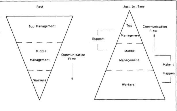
Decision making and problem solving method- ology considering the levels of the organization for conventional and JIT production systems is given by Goddard (1986) as in Figure 1. As can be observed from Figure 1, one of the most important characteristics of a JIT environment is the ability to get all departments involved with everyone else in the organization as well as with themselves. Therefore, it is important for the management to include lower levels in the decision making and problem solving process. Here again, the DSS environment plays an essential role for a successful JIT production system.

In brief, efficiency can be increased in a JIT production system by (i) simplifying the process of communication, (ii) allowing problems to be solved at the point of origin, and (iii) providing

(4)

C. O~uz, C. Dinner / Incorporating just-in-time into a DSS emironment 347

accurate and timely information in order to take corrective action before the process is out of control. Consequently, the advantages of a DSS for JIT production systems can be summarized as follows:

1. DSS can obtain accurate data which is a must in JIT production systems with small time periods.

2. Information gathering process needs to be quick, accurate, and reliable in JIT production systems and this can easily be satisfied in a DSS environment.

3. Communication aspects of a DSS provide the possibility for frequent changes on shop floor together with demand a n d / o r schedule changes in JIT production systems.

4. Interface component provides ease of use of the DSS for the workers on shop floor.

5. Management style of JIT production systems requires incorporation of the workers, team work, and quality circles. These can best be achieved in a DSS environment.

6. Decision making process of a DSS environment gives the opportunity of decision making both from top to bottom (in model base) and from bottom to top (in database) for JIT production systems.

3. A DSS environment for a JIT production sys- tem

In this work, a system that has the characteristics of JIT production systems discussed so far is considered. It is a multi-stage, multi-period, single-line, and single-item production system. A major decision is to determine ULS values, i.e., the number of containers required for each stage in the system. If the environment is stochastic due to demand variations, then the number of required containers may change from time to time and from stage to stage. These decisions are made by supervisors at shop floor level. Conse- quently, if a DSS can be established, supervisors can easily change the number of containers and this type of decisions can be transferred throughout the plant with the help of the DSS. When there is a need to change the number of containers, data can easily be edited using the database. Then results can be observed immediately using model base through interface.

If there is a change in the system, then the model base can be changed by the planning department and these changes can be easily trans- mitted to the shop floor with the help of the DSS. As a result, all changes in the system can be

Past , m

TopManagement

V

J u s t - In - T i m e C o m m u n i c a t i o n

/

orkr 2n

(5)

348 C. O~,uz, C. Dinqer / Incorporating just-in-time into a DSS environment

reflected by the DSS immediately, and the system can be adapted according to these changes. The interaction between the system and the decision maker is established by the DSS with the help of its components, namely the database, the model base, and the interface.

3.1. The database

The data requirement of a JIT production system is huge as in any production system. Fur- thermore, for real-time monitoring and information feedback throughout the system, data has to be collected continuously. Besides, quick response to data evaluation is essential in order to control the production process. This necessitates a database by which the decision maker can edit, view, and use the data. In the database an important point is to identify what data is needed by each of the activities in the system.

For the JIT production system used in this study, the following eleven parameters are identi- fied in order to form the database:

1. Final product demand, 2. Production lead time, 3. Unit load size,

4. Variable processing time, 5. Pulling rate,

6. Container capacity, 7. Inventory holding cost, 8. Backlog cost,

9. Container cost,

10. Unit variable production cost, 11. Annual fixed machine cost.

Among those, to satisfy feasibility conditions, items 1, 2, 4, and 5 must be consistent with each other. Furthermore, items 7, 8, and 10 must also be consistent. In addition, only the final product demand is an external data and in general, it is obtained by a generating process such as forecast- ing.

For the model base, the above required data is generated from a discrete uniform distribution using the predefined parameters so that the decision maker can generate the necessary data by giving its parameters. Data which are dependent on others are generated by considering the functional relationship between the data.

After performing sensitivity analyses on parameters, it is observed that none of the costs, i.e., items 7, 8, 9, 10 and 11, significantly affect

the behavior of the model and hence the system is not sensitive to them. Furthermore, the variable processing time is observed to be sensitive to the capacity of the stages. The upper bounds of the production capacity of the stages are determined by the variable processing time and ULS values of stages. For the final product demand, three cases are considered in the analysis of the system: (i) high demand variability, (ii) medium demand variability, and (iii) low demand variability.

3.2. The interface

An interface is a critical component of any information system and it is a link between the decision maker and the system as well as a link among the component subsystems of the system itself. According to Anthonisse et al. (1988), interaction between the decision maker and the system adds to effectivity, efficiency, and accept- ability. The interface component for the proposed DSS is a processed-oriented interface since the decision maker is led through a sequence of questions. It is assumed that the capabilities of the decision maker will be better utilized via interaction with a process-oriented interface as stated by Bennett (1983).

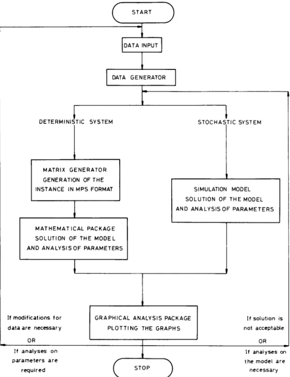
As an interface between the decision maker and the system, a mathematical module is developed. This mathematical module embodies not only the interface but also the database and the model base of the DSS. It includes a data generator which is part of the database and provides the necessary data to the model base. The model base includes a matrix generator together with a mathematical software package when the system is deterministic, and a simulation model when the system is stochastic. The model base (mathematical package or simulation model) solves the given problem and its output is sent to a graphical analysis package. From DSS context, this module provides a medium to the decision maker to enter desired data properties and to obtain graphical results for the solution of the problems. Further- more, this mathematical module permits examination of a large number of alternative data sets, especially for the sensitivity analyses. The relationship between the components of the DSS in the mathematical module is given in Figure 2.

The communication aspect of a DSS can easily be accomplished by the interface component. As

(6)

C. O~uz, C. Dinner / Incorporating just-in-time into a DSS enuironment 349 can be observed from Figure 2, after obtaining

the alternative solutions for the problem, the decision maker can return either to the beginning of the process if some analyses are required for the data or to the model base if it is required to analyze the model used. Also, information obtained from the model base can be sent to the

database to store it and it can be displayed to the decision maker with the help of the interface.

3.3. The model base

Decision making is a process of problem solving and modeling is a vital tool in achieving this.

START )

_ 1

i

1

L

DETERMINISTIC SYSTEM STOCHASTIC SYSTEM

MATRIX GENERATOR GENERATION OF THE INSTANCE IN MPS FORMAT

1

MATHEMATICAL PACKAGE SOLUTION OF THE MODEL AND ANALYSIS OF PARAMETERS

SIMULATION MODEL SOLUTION OF THE MODEL AND ANALYSISOF PARAMETERS

If modifications for

d a t a are necessary OR

If analyses on parameters are

GRAPHICAL ANALYSIS PACKAGE If solution is PLOTTING THE GRAPHS not acceptable

OR ,_, If analyses on

required STOP necessary

(7)

350 C. O~,uz, C. Dinner / Incorporating just-in-time into a DSS encironment

Hence, an adaptive and effective model base component is a must for any DSS. A model base may include several models in which decisions and their quality are specified differently in terms of variables and relations between them. These models can be classified according to their characteristics in performing the decision process. Anthonisse et al. (1988) state that, in the first class, the models are designed to generate decisions such as accounting models, statistical models, and optimization models. In the second class, the model is designed to evaluate decisions. Queueing models and simulation models are ex- amples of that approach.

In the proposed DSS, first a linear programming model is developed for the JIT production system in the model base to analyze the deterministic system with optimization techniques. Then simulation techniques are used when the stochastic parameters are introduced into the system. So, this model base involves models from both two classes.

In previous studies, it is assumed that production kanbans are collected in a stack at the buffer station during the period and then all of the collected production kanbans are sent to the production station at the beginning of the next period in order to trigger production (see Bitran and Chang (1987); Davis and Stubitz (1987); Huang et al. (1983); Kimura and Terada (1981); Philipoom et al. (1987); Rees et al. (1987)). In this study, since a single line production system is considered, i.e. there is no network configuration, it is a natural assumption to send the production kanban to the production station to start production whenever it is detached at the buffer station, if that production station is already waiting for a production order.

By using the model base, unit load size, amount of production, production capacity, inventory level, amount of backlog, and capacity of buffer are determined in terms of containers to minimize the total cost of the system subject to several functional constraints. The system reflects all assumptions and properties of a JIT production system. Furthermore, the following additional assumptions are made for the system:

• buffer capacity is limited with only the maximum demand,

• no partially filled container can move between stations.

3.3.1. Deterministic JIT production system

The model constructed for a deterministic JIT production system described so far is nonlinear in both the objective function and constraints (see O~uz (1988)). But it is computationally restrictive to solve large scale models which have nonlineari- ties in both constraints and the objective function. In this study, the model is transformed into a linear model by taking the ULS as a parameter. The linear model is simpler and much easier to solve. In order to see the effect of ULS, a sensitivity analysis is performed by changing its value. Integer variables constitutes another difficulty in solving this model. In real life, variables will have integral values. In order to remedy computational difficulties, first these constraints are relaxed and a perturbation analysis is performed on the integer variables by maintaining the feasibili- ties of the solution. Then these results are com- pared to see whether they are significantly different or not.

Below, first the definitions related with the model are given and then the transformed model is presented. Definitions. Indices: n: Stage of production (n = 1 , . . . , N). t: Time period (t --- 1 . . . . , T). Parameters:

Hn: Inventory holding cost at stage n per unit per period (S/unit-period).

Sn: Cost of a backlog at a stage per unit per period (S/unit-period).

Kn: Cost of containers including storage and space cost at stage n (S/container). p: Pulling rate (container/period).

Dr: Demand of final product in period t (unit).

Ln: Production lead time at stage n.

U~n: Unit variable production cost at stage n at time period t (S/unit-period).

AFCn: Annual fixed machine cost rate for stage n (S/period).

an: Variable processing time for stage n (time unit/unit).

Decision Variables:

07: Net accumulated number of empty containers at stage n in time period t, i.e., production order quantity.

(8)

C. O~uz, C Dinner / Incorporating just-in-time into a DSS environment 351

PF: Production amount of stage n in time period t (number of full containers).

Mn: Unit load size at stage n.

cn: Production capacity of stage n.

Wt": N u m b e r of units of item remaining in a partially filled container at stage n in time period t.

I~: Number of full containers in buffer at stage n in time period t (amount of inventory carried).

BT: Number of empty containers in buffer at stage n in time period t (amount of backlog).

X": Number of containers in buffer at stage n.

Model.

(i) Objective function is to minimize the total cost:

min TC = E ( Ut ~ + AFC na ~) M n P f + Y', Utn Wt n

tl,t tt,l

+ E H"M"It" + E S " M ' B ~ + E K " X " . n , l n , t n

(ii) Constraints:

(1) M a x i m u m possible production quantity: (a) Total production must not exceed capacity (in terms of units):

Mnpt" + I, Vt~ - M~C~ <~ O V t , V n .

(b) Total production must not exceed the total in-process inventory of the preceding stage (in terms of units): - - l t . ¢ n + l D n + l l i f t + 1, MnP~ + Wi ~ ~,, ~_L,+~ ~< M ~+ n = l . . . N - l , - M n + l I n+l Mn+lB~+11 Mnptn+Wt n t - 1 + - - M " + 1Ptn_~ l_L.+l ~< 0, t = 2 . . . T, n = l . . . N - l , M N p f f + W N ~ X N + I , M N p , N+wtN<~IN+I', t = 2 , . . . , r .

(c) Production must not exceed the empty buffer amount (buffer s i z e - on-hand inventory) (in terms of containers):

P ~ ' - X n ~< -I~' Vn,

P t - X ~ + I [ ' _ I < ~ O , t = 2 . . . T, Vn.

(2) Balance equations for the number o f units o f

items remaining in a partially filled container:

W11 = M 1 0 ~ - D1,

W / = W t l 1 + M I O ] - D t , t = 2 . . . . , T ,

Wt" = Wt n , + M " O ~ - M ' - I P t " - ' ,

n = 2 , . . . , N , Vt.

(3) Net inventory balance equations (in terms of units): M1B~ - M I I 1 + M ' P ~ _ L, = D 1 - M l i I ' M ' B ] - M1B]_, - M I # + Mtl,'_l + M1p,1L~ = Dr, t = L 1 + 1 . . . T, M " B ~ - M " I ~ + Mnp~_L. - M " - ' P ~ - I _ W ? - I = - M n I g , n = 2 , . . . , N , MnB~ - M~B~- 1 - MnI~ ' + M"I]_~ + Mnpt~_L. - M n - l p t n - l _ _ w t n - l = O , t = L " + l . . . T, n = 2 . . . N.

(4) Production order quantity balance equations (in terms of units) (production order quantity = demand (or total production quantity of the succeeding s t a g e ) + backorder from previous time p e r i o d - on-hand inventory from previous time p e r i o d - u n i t s produced in a partially filled container in previous time period):

M I o ~ = D 1 - M I I 1, M ' O ] - M I B ] _ 1 + M l l t ' - - 1 + W/_, = D r t = 2 , . . . , T , M ~ O ~ _ M ~- 1p~ -1 _ W(' -1 = _ M n I ~ , n = 2 , . . . , N , M " O ~ - M n B ~ ' I + M"It_ 1 - M " - 1 P t "-1 + Wt~l - W t ' - l = O , t = 2 . . . . , T , n = 2 . . . N .

(5) Bounds for buffer."

X " < ~ m a x ( D t : t = l , . . . , T ) / M ~ V n ,

X ' > ~ m i n ( D t : t = l . . . T ) / M ~ V n .

(6) Upper bound for number o f units remaining

in a partially filled container:

(9)

352 C. O~,uz, C. Dinner / Incorporating just-in-time into a DSS environment

(7) Lower and upper bounds for capacity:

C n >~p Vn,

C" <~ 1 / ( a " M ") Vn.

(8) Nonnegativity constraints:

O f , Wt">~O V t , n.

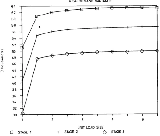
Optimization and statistical techniques are used to solve and to analyze the above model. Production lead time is taken as zero to reduce the computational difficulty. Sensitivity analysis is carried out on the d e m a n d and ULS to see the effects of these p a r a m e t e r s on the response of the model. To eliminate the bias and to incorporate true randomness of data, twenty statistically independent runs are g e n e r a t e d and their average values are considered as the result for each problem. In this case, there exist 10 × 3" different data patterns to be examined where n de- notes the n u m b e r of stages in the system. Since as n increases the n u m b e r of problems also increases, n is taken equal to 3 to observe the gross effect of the production system. T h e results can easily be extended to a system with n ~> 4 by

adding extra intermediate stages. When the total cost function is examined, it is seen that the value of the total cost function is very sensitive to a change in the ULS value from 1 to 2. For further increases in the ULS value, the change in the value of the total cost function reduces. This trend is the same in all stages for all d e m a n d types. A typical result of the deterministic system is given in Figure 3. A n o t h e r result, observed from the solutions of perturbing the variables to integer values, indicates that the relaxed LP solution differs from the optimal solution by at most 4 percent.

3.3.2. Stochastic JIT production system

Since it is computationally hard to incorporate uncertainty into the constructed model, a simulation model is developed for the stochastic system. In addition, the need for the dynamic interactions between decisions and among the variables together with the long time horizon makes it mean- ingful to use simulation instead of optimization techniques. But due to its descriptive nature, it is very hard to conduct an optimization with a simulation model. Simulation shows only

0 U ~ tl.I < 64 62 60 58 54

-

52 ~ 50

-

4B - /

46 - 44 - 42 - 40 36 34 32 30 [ ] STAGE I

HIGH DEMAND VARIANCE

[] El O .~.

I I I I

0

0 -I^

0

l I I I I I I I

3 5 7 9

UNIT LOAD SIZE

4- STAGE 2 ~ STAGE 3

(10)

UJ N U3~ C O I.t.I r n , . v t..tl 43 42 /.,1 /*0 39 38 37 36

C. O~uz, C. Dinner / Incorporating just-in-time into a DSS environment D (20,/*0)AND B ( 3 0 , 5 0 )

I I I I I I I I I

1 3 5 7 9

UNIT LOAD SIZE

STAGE 1 + STAGE 2 ~ STAGE 3

Figure 4. Results for medium demand variability and buffer capacity greater than mean demand in a stochastic system D (20,/.,0) AND B ( 3 0 , 3 0 ) /.,5 --r O t ) o o LLI 0 W < /.,4 43 /.,2 /.,,1 40 39 38 37 36 35 34 _I _I _I _I ₁ _I _I _I _I 1 3 5 7 9

UNIT LOAD SIZE

O STAGE 1 + STAGE 2 ~ STAGE 3

Figure 5. Results for medium d e m a n d variability and buffer capacity at mean demand in a stochastic system

(11)

354 C. O~uz, C. Dinner / Incorporating just-in-time into a DSS environment the relationship between various components of

the system and predicts the performance of the system under different operating policies. In short, it evaluates the system numerically over a time period.

While simulating the system, the production lead time is no longer taken to be zero, but it is changed in an interval as a function of variable processing time and is generated from the uniform distribution. Furthermore, the buffer capacity is limited with only the maximum demand, i.e. the buffer capacity is unlimited in the deterministic system. Therefore, in order to see the effect of the buffer capacity on the system, the buffer capacity is taken as a parameter in the simulation. Three cases are considered for the buffer capacity. In the first case, the buffer capacity is generated so that the mean value is 50% less than the mean demand. In the second case, the buffer capacity is equal to the mean demand. In the final case, the buffer capacity is generated where its mean value is 50% greater than the mean demand value.

In this part of the study, by taking three stages, three levels of demand, and three levels of buffer

k - u 3 8 O b J r ~ h i E O 3 o v 46 45 4 4 - 43 42 41 40 39 I 38 ~ 37 - 36 1 I I I 3 [ ] STAGE 1

together with ten ULS values, 252 different problem structures are simulated. For each problem structure, ten independent runs are conducted and the average of ten different runs is analyzed in the simulation.

The simulation model reflects the production system's processes and characteristics, generates data needed by the decision logic and answers questions such as:

• what happens if ULS values change? • how much must be produced to minimize in-process inventories?

• how will the cost function behave under capacity a n d / o r ULS changes?

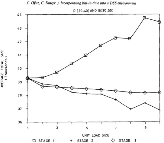
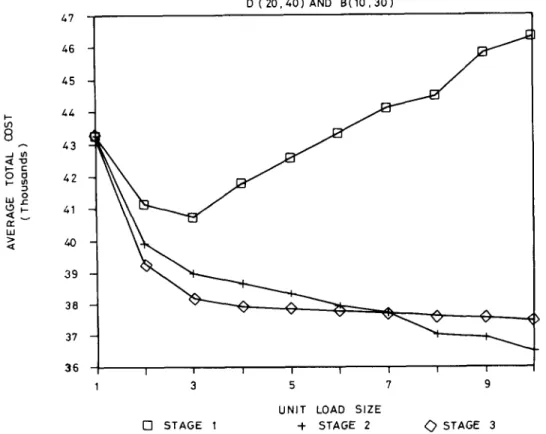
The main point in this simulation is to determine the value of the ULS and to get an idea about the long-run behavior of the system. A similar analysis is carried out for the simulation as for the deterministic system. The results show that as buffer capacity increases, the cost function becomes concave. This result supports the solution of the deterministic system with respect to the buffer capacity. As can be seen from Figures 4, 5, and 6, this structure is stronger at the first stage, which produces the final product, com- D ( 2 0 , 4 0 ) AND B ( 1 0 , 3 0 )

I I l I [

5 7 9

UNIT LOAD SIZE

-I- STAGE 2 ~ STAGE 3

(12)

C. O~uz, C. Dinqer / Incorporating just-in-time into a DSS environment 355

pared to the previous stages. This means that the first stage is more sensitive to a change in the buffer capacity. Since this is the stage that di- rectly affects the final product; hence the cus- tomers and the buffer capacity should be care- fully determined. One can also observe that, as in the deterministic system, the slope of the total cost function becomes flatter as the ULS values increase. This shows that the cost function is very robust after some threshold value of the ULS. It is interesting to note that when the buffer capacity is tightly constrained, the best value of ULS appears to be 3 which is greater than the ideal one unit. As the buffer capacity increases the best value of ULS approaches to one unit. These observations can also be deduced from Figures 4, 5, and 6.

4. Conclusions

In this paper, the incorporation of a JIT production system into a DSS environment together with the advantages of such an incorporation are discussed. The proposed DSS environment is also provided for the JIT production system.

As explained in the main body of the paper, DSS has many advantages for JIT production systems. It makes the communication easier which helps a JIT production system to achieve its requirements and ultimate goal. Furthermore, the involvement of shop floor to management which is a necessity for a JIT production system can be better attained with a DSS environment. In addition, data collection can be easier, quicker and more accurate in this environment. This increases the efficiency and the effectiveness of a JIT production system since time periods are very short in such systems.

Another advantage of a DSS environment for a JIT production system is to utilize a model base. For instance in this study, the decision maker has the opportunity to treat the system both as deterministic and stochastic. Analysis of a stochastic system may require a substantial computational effort and the decision maker may prefer to analyze the .deterministic system as an approximation to the stochastic system. Then, having a feeling on how good this deterministic approximation is, the decision maker chooses the appropriate model. On the other hand, the deci-

sion maker may want to use the long-run results obtained from the simulation study in the analyses of the deterministic system. Therefore by having these results in its database, the DSS provides an environment to the decision maker to perform these analyses with ease.

Also, this study analyzes the system according to the changes in ULS values. These values can be updated according to demand changes in the system. This requires many interactions among the system, shop floor, and every level of the organization. DSS provides an environment that efficiently handles such interactions. In addition, a DSS environment generates several solution alternatives for the problems of the decision maker. A final decision is obtained through DSS after analyses on the alternative solutions with the preference policy of the decision maker. For example, in the simulation study, there are different ULS values with different costs and since there is no optimization in simulation, a solution which seems inferior to another solution may be selected by the decision maker. But this solution may be preferred by the decision maker according to the conditions on the shop floor and his accumulated knowledge of the system. Accord- ingly, one of the alternative solutions may be selected by the decision maker using his experi- ence.

In brief, the DSS helps the decision maker in the decision making process by increasing the productivity and the profitability of the system which, as in any production system, is the major goal in a JIT production system.

References

Anthonisse, J.M., Lenstra, J.K., and Savelsbergh, M.W.P. (1988), "Behind the screen: DSS from an OR point of view", CWI Report OS-R8805, Centre for Mathematics and Computer Science, Amsterdam.

Bennett, J.L. (1983). Building Decision Support Systems, Addi- son-Wesley, Reading MA.

Bitran, G.R., and Chang, L. (1987), " A mathematical programming approach to a deterministic kanban system", Management Science 33/4, 427-441.

Conway, R., Maxwell, W., Clain, J.O., and Thomas, L.J. (1988), "The role of work-in-process inventory", Opera- tions Research 36/2, 2297241.

Davis, W.J., and Stubitz, S.J. (1987), "Configuring a kanban system using a discrete optimization of multiple stochastic responses", International Journal of Production Research 25/5, 721-740.

(13)

356 C. O~uz, C. Dinner / Incorporating just-in-time into a DSS environment

Eom, H.B., and Lee, S.M. (1990), "Decision Support Systems applications research: A bibliography (1971-1988)", Euro- pean Journal of Operation Research 46/3, 333-342. Finch, B.J., and Cox, J.F. (1986), "An examination of Just-In-

Time management for the small manufacturer: With an illustration", International Journal of Production Research 24/2, 329-342.

Goddard, W.E. (1986), Just-In-Time: Surviving by Breaking Tradition, Oliver Wight Limited Publications.

Gray, P., and Lenstra, J.K. (1988), "Special focus and Deci- sion Support Systems (DSS)", Operations Research 36/6, 823-825.

Huang, P.Y., Rees, L.P., and Taylor III, B.W. (1983), "A simulation analysis of the Japanese Just-In-Time technique (with kanbans) for a multiline, multistage produc- tion system", Decision Science 14, 326-343.

Kimura, O., and Terada, H. (1981), "Design and analysis of pull system, a method of multi-stage production control", International Journal of Production Research 19/3, 241- 253.

Methlie, L.B., and Sprague, R.H. (eds.) (1986), Knowledge Representation for Decision Support Systems, Elsevier, Am- sterdam.

Mittra, S.S. (1986), Decision Support Systems: Tools and Tech- niques, Wiley, New York.

Monden, Y. (1981a), "What makes the Toyota production system really tick?", Industrial Engineering 13/1, 36-46. Monden, Y. (1981b), "Adaptable kanban system helps Toyota

maintain Just-In-Time production", Industrial Engineering 13/5, 29-45.

Monden, Y. (1983), Toyota Production System, Industrial En- gineering and Management Press.

O~uz, C. (1988), "Design and analysis of Just-In-Time Pro- duction Systems", Unpublished Master's Thesis, Bilkent University, Ankara.

Philipoom, P.R., Rees, L.P., Taylor III, B.W., and Huang, P.Y. (1987), "An investigation of the factors influencing the number of kanbans required in the implementation of the JIT technique with kanbans", International Journal of Production Research 25/3, 457-472.

Rees, L.P., Philipoom, P.R., Taylor III, B.W., and Huang, P.Y. (1987), "Dynamically adjusting the number of kanbans in a Just-In-Time production system using estimated values of lead time", liE Transactions 19/2, 199-207. Schonberger, R.J. (1982), "Some observations on the advan-

tages and implementations issues of Just-In-Time produc- tion systems", Journal of Operations Management 3/1, 1-11.

Schonberger, R.J. (1983), "Selecting the right manufacturing inventory system: Western and Japanese approaches", Production and Inventory Management 24/2, 33-44. Schonberger, R.J., and Schniederjans, M.J. (1984), "Reinvent-

ing inventory control", Interfaces, 14/3, 76-83.

Sprague Jr., R.H. (1986), "A framework for the development of Decision Support Systems", in: R.H. Sprague Jr. and H.J. Watson (eds.), Decision Support Systems: Putting The- pry into Practice, 7-32,

Trevino, J., and Mc Ginnis, L.F. (1987), "Design procedures for Just-ln-Time production systems", 1FORS 1987, Buenos Aires, August, 10-14.