COMPUTATIONS
a thesis
submitted to the department of electrical and
electronics engineering
and the institute of engineering and science
of bilkent university
in partial fulfillment of the requirements
for the degree of
master of science
By
Ali Rıza Bozbulut
September 2005
Prof. Dr. Levent G¨urel (Supervisor)
I certify that I have read this thesis and that in my opinion it is fully adequate, in scope and in quality, as a thesis for the degree of Master of Science.
Prof. Dr. Ayhan Altınta¸s
I certify that I have read this thesis and that in my opinion it is fully adequate, in scope and in quality, as a thesis for the degree of Master of Science.
Assoc. Prof. Dr. Tu˘grul Dayar
Approved for the Institute of Engineering and Science:
Prof. Dr. Mehmet Baray
Director of the Institute Engineering and Science
IMPLEMENTATIONS FOR ELECTROMAGNETIC
COMPUTATIONS
Ali Rıza Bozbulut
M.S. in Electrical and Electronics Engineering Supervisor: Prof. Dr. Levent G¨urel
September 2005
Multilevel fast multipole algorithm (MLFMA) is an accurate frequency-domain electromagnetics solver that reduces the computational complexity and memory requirement significantly. Despite the advantages of the MLFMA, the maximum size of an electromagnetic problem that can be solved on a single pro-cessor computer is still limited by the hardware resources of the system, i.e., memory and processor speed. In order to go beyond the hardware limitations of single processor systems, parallelization of the MLFMA, which is not a trivial task, is suggested. This process requires the parallel implementations of both hardware and software. For this purpose, we constructed our own parallel com-puter clusters and parallelized our MLFMA program by using message-passing paradigm to solve electromagnetics problems. In order to balance the work load and memory requirement over the processors of multiprocessors systems, efficient load balancing techniques and algorithms are included in this parallel code. As a result, we can solve large-scale electromagnetics problems accurately and rapidly with parallel MLFMA solver on parallel clusters.
Keywords: Parallelization, Load Balancing, Partitioning, Optimization, Parallel Computer Cluster.
ELEKTROMANYET˙IK HESAPLAMALARI ˙IC
¸ ˙IN
PARALEL DONANIM VE YAZILIM UYGULAMALARI
Ali Rıza Bozbulut
Elektrik ve Elektronik M¨uhendisli˘gi, Y¨uksek Lisans Tez Y¨oneticisi: Prof. Dr. Levent G¨urel
Eyl¨ul 2005
C¸ ok seviyeli hızlı cok kutup y¨otemi (C¸ SHC¸ Y) frekans alanında hassas sonu¸clar veren bir elektromanyetik ¸c¨oz¨uc¨us¨ud¨ur; bu ¸c¨oz¨uc¨u hesapsal karma¸sıklı˘gı ve bellek gereksinimi olduk¸ca azaltmı¸stır. C¸ SHC¸ Y’nin t¨um bu yararlarına kar¸sın, tek i¸slemcili bilgisayarların donanım kaynakları, ¨orne˘gin bellek miktarı ve i¸slemci hızı, ¸c¨oz¨ulebilen elektromanyetik problemlerin b¨uy¨ukl¨u˘g¨un¨u kısıtlamaktadır. Tek i¸slemcili sistemlerin bu kısıtlamalarını a¸sabilmek i¸cin, C¸ SHC¸ Y’nin par-alelle¸stirilmesi ¨onerilmi¸stir. C¸ SHC¸ Y’nin paralelle¸stirilmesi kolay bir i¸slem de˘gildir, bu i¸slemin yapılabilmesi i¸cin paralel donanım ve yazılım alanında yo˘gun emek ve deneyim gerekmektedir. Elektromanyetik problemleri paralel ortamda ¸c¨ozebilmek icin kendi paralel bilgisayar k¨umemizi kurduk ve C¸ SHC¸ Y kodumuzu paralelle¸stirdik. Paralel bilgisayarlar ¨uzerindeki i¸s y¨uk¨un¨u ve bellek kullanımını dengeleyen verimli y¨uk dengeleme algoritmalarını ve y¨ontemlerini paralel kodu-muza yerle¸stirdik. S¸u anda, paralel C¸ SHC¸ Y ¸c¨oz¨uc¨um¨uzle geli¸sig¨uzel ¸sekilli ¸cok b¨uy¨uk elektromanyetik problemleri paralel bilgisayar k¨umeleri ¨uzerinde ¸cok kısa bir zamanda ¸c¨ozebilmekteyiz.
Anahtar s¨ozc¨ukler : Paralelle¸stirme, Y¨uk Dengelemesi, Y¨uk Da˘gıtımı, Optimizasyon, Paralel Bilgisayar K¨umesi.
I gratefully thank my supervisor Prof. Dr. Levent G¨urel for his supervision and guidance throughout the development of my thesis.
I also thank Prof. Dr. Ayhan Altınta¸s and Assoc. Prof. Dr. Tu˘grul Dayar for reading and commenting on my thesis.
I also thank all graduate students of Bilkent Computational Electromagnetics Laboratory for their strong support in my studies.
I express my sincere gratitude to TUBITAK for allowing access to their high performance computing cluster, ULAKBIM, on which part of the computations for the work described in this thesis was done.
1 Introduction 1
1.1 Motivation . . . 1
1.2 Parallel Computer Systems and Parallelization Techniques . . . 3
1.2.1 Communicational Model of Parallel Computer Systems . . . 4
1.2.2 Control Structure of Parallel Computer Systems . . . 7
1.3 Parallelization Basics and Concepts . . . 9
1.4 An Overview to the Parallelization of MLFMA . . . 12
2 Parallel Environments 14 2.1 32-Bit Intel Pentium IV Cluster . . . 15
2.1.1 Hardware Structure of 32-Bit Intel Pentium IV Cluster . . 15
2.1.2 Software Structure of 32-Bit Intel Pentium IV Cluster . . . 17 2.2 Hybrid 32-Bit Intel Pentium IV and 64-Bit Intel Itanium II Cluster 20
2.3 Proposed 64-Bit AMD Opteron Cluster . . . 23
2.4 ULAKBIM Cluster . . . 26
3 Parallelization of MLFMA 29 3.1 Adaptation of MLFMA into Parallel System . . . 29
3.2 Partitioning Techniques . . . 30
3.3 Partitioning in Parallel MLFMA . . . 32
3.3.1 Partitioning of Block Diagonal Preconditioner . . . 32
3.3.2 Partitioning of MLFMA Tree Structure . . . 34
3.4 Load Balancing in Parallel MLFMA . . . 35
3.4.1 Load Balancing of Near-field Interactions Related Opera-tions and Structures . . . 40
3.4.2 Load Balancing of Far-field Interactions Related Operations and Structures . . . 40
4 Results of Load Balancing Techniques 42 4.1 Sphere Geometry . . . 43
4.1.1 Time and Memory Profiling Results . . . 44
4.1.2 Speedup, Memory Gain, and Scaling Results . . . 51
4.2 Helicopter Geometry . . . 61
4.2.1 Time and Memory Profiling Results . . . 62
1.1 Shared-address-space architecture models: (a) uniform-memory-access multiprocessors system (UMA) model and (b)
non-uniform-memory-access multiprocessors system (NUMA) model . . . 5
1.2 Message-passing multicomputer model . . . 6
1.3 Control architectures: (a) single instruction stream, multi-ple data stream (SIMD) model and (b) multimulti-ple instruc-tion stream, multiple data stream (MIMD) model . . . 8
1.4 Typical speedup curves . . . 11
2.1 Typical Beowulf system . . . 16
2.2 File system structure of a Beowulf cluster . . . 17
2.3 Generating a parallel MLFMA executable . . . 19
2.4 Run of a parallel program on homogenous Beowulf cluster . . . . 20
2.5 Execution of a parallel program on hybrid Beowulf cluster . . . . 21
2.6 Mountings in the hybrid cluster . . . 22
2.7 Performance comparison of different processors with pre-solution part of sequential MLFMA . . . 24
2.8 Performance comparison of different processors with matrix-vector multiplication in the iterative solver part of sequential MLFMA . 25 2.9 Performance comparison of different processors with pre-solution
part of parallel MLFMA . . . 27
2.10 Performance comparison of different processors with matrix-vector multiplication in the iterative solver part of parallel MLFMA . . . 27
3.1 (a) One-dimensional partitioning of an array (b) two-dimensional partitioning of an array . . . 31
3.2 Extraction of preconditioner matrix . . . 33
3.3 Partitioning of preconditioner matrix . . . 33
3.4 Partitioning of MLFMA tree . . . 34
3.5 Structure of forward load balancing algorithm for the memory . . 38
3.6 Structure of backward load balancing algorithm for the memory . 39 3.7 Memory calculations for far-field related arrays . . . 41
4.1 Electromagnetic scattering problem from a PEC sphere . . . 43
4.2 Memory usage of near-field interactions related arrays for sphere with 1.5 mm mesh when load balancing algorithms are not applied 45 4.3 Memory usage of near-field interactions related arrays for sphere with 1.5 mm mesh when load balancing algorithms are applied . . 45
4.4 Memory usage of far-field interactions related arrays for sphere with 1.5 mm mesh when load balancing algorithms are not applied 46 4.5 Memory usage of far-field interactions related arrays for sphere with 1.5 mm mesh when load balacing algorithms are applied . . 46
4.6 Peak memory usage in the modules of MLFMA for sphere with 1.5 mm mesh when load balancing algorithms are not applied . . . . 47 4.7 Peak memory usage in the modules of MLFMA for sphere with 1.5
mm mesh when load balancing algorithms are applied . . . 47 4.8 Pre-solution time for sphere with 1.5 mm mesh when load
balanc-ing algorithms are not applied . . . 49 4.9 Pre-solution time for sphere with 1.5 mm mesh when load
balanc-ing algorithms are applied . . . 49 4.10 Matrix-vector multiplication time profiling for sphere with 1.5 mm
mesh when load balancing algorithms are not applied . . . 50 4.11 Matrix-vector multiplication time profiling for sphere with 1.5 mm
mesh when load balancing algorithms are applied . . . 50 4.12 Memory scale plots of three different sphere meshes for array
struc-tures, which are related with near-field computations (load balanc-ing algorithms are not applied) . . . 52 4.13 Memory scale plots of three different sphere meshes for array
struc-tures, which are related with near-field computations (load balanc-ing algorithms are applied) . . . 52 4.14 Memory gain plots of three different sphere meshes for array
struc-tures, which are related with near-field computations (load balanc-ing algorithms are not applied) . . . 53 4.15 Memory scale plots of three different sphere meshes for array
struc-tures, which are related with near-field computations (load balanc-ing algorithms are applied) . . . 53 4.16 Memory scale plots of three different sphere meshes for array
struc-tures, which are related with far-field computations (load balancing algorithms are not applied) . . . 54
4.17 Memory scale plots of three different sphere meshes for array struc-tures, which are related with far-field computations (load balancing algorithms are applied) . . . 54 4.18 Memory gain plots of three different sphere meshes for array
struc-tures, which are related with far-field computations (load balancing algorithms are not applied) . . . 55 4.19 Memory gain plots of three different sphere meshes for array
struc-tures, which are related with far-field computations (load balancing algorithms are applied) . . . 55 4.20 Time scale plots of three different sphere meshes for the
computa-tions of near-field interaccomputa-tions (load balancing algorithms are not applied) . . . 56 4.21 Time scale plots of three different sphere meshes for the
compu-tations of near-field interactions (load balancing algorithms are applied) . . . 56 4.22 Speedup plots of three different sphere meshes for the
computa-tions of near-field interaccomputa-tions (load balancing algorithms are not applied) . . . 57 4.23 Speedup plots of three different sphere meshes for the
computa-tions of near-field interaccomputa-tions (load balancing algorithms are ap-plied) . . . 57 4.24 Time scale plots of three different sphere meshes for the
matrix-vector multiplication (load balancing algorithms are not applied) . 58 4.25 Time scale plots of three different sphere meshes for the
matrix-vector multiplication (load balancing algorithms are applied) . . . 58 4.26 Speedup plots of three different sphere meshes for the
4.27 Speedup plots of three different sphere meshes for the matrix-vector multiplication (load balancing algorithms are applied) . . . 59 4.28 PEC helicopter model . . . 61 4.29 Memory usage of arrays structures which are related with near-field
interactions for helicopter with 1.5 cm mesh when load balancing algorithms are not applied . . . 63 4.30 Memory usage of arrays structures which are related with near-field
interactions for helicopter with 1.5 cm mesh when load balancing algorithms are applied . . . 63 4.31 Memory usage of arrays structures which are related with far-field
interactions for helicopter with 1.5 cm mesh when load balancing algorithms are not applied . . . 64 4.32 Memory usage of arrays structures which are related with far-field
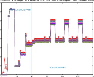
interactions for helicopter with 1.5 cm mesh when load balancing algorithms are applied . . . 64 4.33 Peak memory usage in the modules of MLFMA for helicopter with
1.5 cm mesh when load balancing algorithms are not applied . . . 65 4.34 Peak memory usage in the modules of MLFMA for helicopter with
1.5 cm mesh when load balancing algorithms are applied . . . 65 4.35 Pre-solution time for helicopter with 1.5 cm mesh when load
bal-ancing algorithms are not applied . . . 66 4.36 Pre-solution time for helicopter with 1.5 cm mesh when load
bal-ancing algorithms are applied . . . 66 4.37 Matrix-vector multiplication-time profiling for helicopter with 1.5
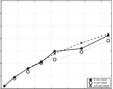
4.38 Matrix-vector multiplication-time profiling for helicopter 1.5 cm mesh when load balancing algorithms are applied . . . 67 4.39 Memory scale plots of three different helicopter meshes for array
structures, which are related with near-field interactions (load bal-ancing algorithms are not applied) . . . 69 4.40 Memory scale plots of three different helicopter meshes for array
structures, which are related with near-field interactions (load bal-ancing algorithms are applied) . . . 69 4.41 Memory gain plots of three different helicopter meshes for array
structures, which are related with near-field interactions (load bal-ancing algorithms are not applied) . . . 70 4.42 Memory gain plots of three different helicopter meshes for array
structures, which are related with near-field interactions (load bal-ancing algorithms are applied) . . . 70 4.43 Memory scale plots of three different helicopter meshes for array
structures, which are related with far-field interactions (load bal-ancing algorithms are not applied) . . . 71 4.44 Memory scale plots of three different helicopter meshes for array
structures, which are related with far-field interactions (load bal-ancing algorithms are applied) . . . 71 4.45 Memory gain plots of three different helicopter meshes for array
structures, which are related with far-field interactions (load bal-ancing algorithms are not applied) . . . 72 4.46 Memory gain plots of three different helicopter meshes for array
structures, which are related with far-field interactions (load bal-ancing algorithms are applied) . . . 72
4.47 Time scale plots of three different helicopter meshes for the com-putations of near-field interactions (load balancing algorithms are not applied) . . . 73 4.48 Time scale plots of three different helicopter meshes for the
com-putations of near-field interactions (load balancing algorithms are applied) . . . 73 4.49 Speedup plots of three different helicopter meshes for the
compu-tations of near-field interactions (load balancing algorithms are not applied) . . . 74 4.50 Speedup plots of three different helicopter meshes for the
com-putations of near-field interactions (load balancing algorithms are applied) . . . 74 4.51 Time scale plots of three different helicopter meshes for the
matrix-vector multiplication (load balancing algorithms are not applied) . 75 4.52 Time scale plots of three different helicopter meshes for the
matrix-vector multiplication (load balancing algorithms are applied) . . . 75 4.53 Speedup plots of three different helicopter meshes for the
matrix-vector multiplication (load balancing algorithms are not applied) . 76 4.54 Speedup plots of three different helicopter meshes for the
4.1 Sphere geometries, which were used in the profiling measurements 43 4.2 Helicopter geometries, which were used in the profiling measurements 61
Introduction
1.1
Motivation
Computational electromagnetics (CEM) deals with the solution of real-life elec-tromagnetic problems in the computer simulation environment. In our studies, we mainly focus on two types of of these real-life problems: Radiation problems and scattering problems.
In radiation problems, we aim to model and simulate the electromagnetic field radiation from a source which is placed on a conducting body e.g., far-field radiation modeling of an antenna. On the other hand; in scattering problems, our goal is focused on the simulation of scattered electromagnetic field, which is transmitted from a conducting object after the illumination of this object with an external electromagnetic radiation source e.g., radar cross section (RCS) profile computations of a helicopter.
In order to solve these kinds of problems accurately, many researchers in the field of computational electromagnetics use the method of moments (MoM). MoM is based on the discretization of electromagnetic integral equation into a matrix equation. The memory requirement and computational complexity of this method are both in the order of O(N2
), where N is number of unknowns; 1
because of such high computational complexity and memory requirement, the size of the electromagnetic problem that is solvable with this method is very limited. Even today’s computers can not satisfy the memory requirement of a MoM based electromagnetic simulation program for the solution of a moderate size electromagnetic problem which might have 50000–60000 unknowns—a MoM based program needs at least 20 GBytes of memory to solve a 50000 unknowns electromagnetic scattering problem.
In 1993, Vladimir Rokhlin proposed the fast multipole method (FMM) for the solution of electromagnetic scattering problems in three dimensions (3-D) [1]. FMM reduces the complexity of matrix-vector computations and memory require-ment to O(N1.5), where N is the number of unknowns. After the proposal of this
new method, multilevel versions of FMM were proposed [2]. Weng Cho Chew introduced a new view to multilevel FMM by using translation, interpolation and anterpolation (adjoint interpolation) concepts. This new multilevel FMM approach was renamed as multilevel fast multipole algorithm (MLFMA). Chew and his group reduced the computational complexity and memory requirement of FMM to O(N log N ) with the new MLFMA [3].
With this new algorithm, MLFMA, people started to solve large scattering problems, which are not solvable with MoM. Despite the advantages of MLFMA in terms of memory and computational time, people have to use very effective supercomputers to solve large scattering problems, which correspond to the num-ber of unknowns in the order of one million. Using the supercomputers for the solution of large electromagnetic scattering problems is very costly; because of that reason and to overcome the hardware limitations of supercomputers, re-searchers shifted their studies into the parallelization process with message pass-ing paradigm. In 2003, research group of Weng Cho Chew at University of Illinois computed bistatic RCS of an aircraft, whose dimensions are not scaled down, at 8 GHz with the parallel implementation of MLFMA [4]. This computation corre-sponds to the solution of 10.2 million unknown dense matrix equations and this is a turning point in CEM area. After that achievement, many research groups in CEM community started to work on parallel implementations of MLFMA. Our group has been working on parallel MLFMA since 2001 and we have developed
our own parallel MLFMA code in order to solve very large scattering problems on Beowulf parallel PC clusters. Now, we can solve 1.3 million unknowns helicopter problem with our parallel MLFMA code on a 32 nodes parallel PC cluster. Our studies are still continuing and our aim is to achieve the computation capabil-ity to solve much larger electromagnetic scattering problems, which might have number of unknowns greater than 3–3.5 millions.
1.2
Parallel Computer Systems and
Parallelization Techniques
In this part, we present an overview of various architectural basics and concepts which lay behind the parallel computer systems. These basics are detailed ac-cording to two categories: We give the details of hardware structure choices that most of parallel computers are based, and then, we introduce the programming models in order to use these hardware structures effectively.
From hardware structure point of view, parallel computer platforms can be classified with respect to the communicational model that they use. On the other side, from software point of view, parallel systems can be grouped according to the control structures in order to program them. So, in the following two subsections we mainly focus on the these issues:
1. Communicational Model of Parallel Computer Systems 2. Control Structure of Parallel Computer Systems
1.2.1
Communicational Model of Parallel Computer
Systems
Parallel computers need to exchange data during parallel tasks. There are two primary ways to do this data exchange between parallel jobs: By using shared-address-space systems or with the usage of sending messages between tasks. De-pending on these mentioned communicational approaches, parallel computer plat-forms can be grouped in two groups:
Shared-address-space platforms: This type of parallel systems have single memory addressing space, which supports the access to the memory from all the processors of the system. These parallel platforms are also sometimes referred to as multiprocessors [5].
Message-passing platforms: In this approach, every processing unit or pro-cessor of these platforms has its own address space for its memory. So, none of the processing units can reach other processing units’ data directly. Because of this reason, processing units send and receive messages between themselves in order to do data exchange. Since these systems are mostly based on the connection of separate single processor computers, they are sometimes called as multicomputers [6].
Shared-Address-Space Platforms
Memory in these parallel computers might be common to all the processors or it may be exclusive to each processor. If the time required to access memory address on the system is equal for all processors, this shared-address parallel computer is classified as uniform memory access (UMA) computer. On the other hand, if this access duration changes from one processor to the another processor, this system is categorized as non-uniform access (NUMA) parallel computer system. UMA and NUMA architectures are depicted in the Fig. 1.1:
IN T E R C O N N E C T IO N N E T W O R K (b) P M P M … …… ……… ……… …… … …… P M
SHARED -ADDRESS -SPACE
IN T E R C O N N E C T IO N N E T W O R K P M P P M M (a) …… … … …… ……… …… … …… … …… … … …… ……… ……… … P : PROCESSOR M : MEMORY
Figure 1.1: Shared-address-space architecture models: (a) uniform-memory-access multiprocessors system (UMA) model and (b) non-uniform-memory-uniform-memory-access multiprocessors system (NUMA) model
Programming in these systems is very attractive with respect to message-passing multicomputers; because, the data is shared among all the processors. Therefore, the programmer need not worry about how to update the data if there is a change during the execution of parallel task in these systems. Generally, shared address space computers are programmed using special parallel program-ming languages, which are extensions of existing sequential languages; e.g. High Performance Fortran 90 (HPF90) is derived from Fortran 90 in order to pro-gram the multiprocessors in parallel with Fortran language. In addition to these parallel languages, threads can be used for programming these platforms.
Despite these advantages in programming these systems, generally multicom-puters are very expensive with respect to off-the-shelf single processor comput-ers. Moreover, the development stages of these platforms take a lot of time and therefore, these platforms are usually superseded by single processors, which
have been regularly upgraded. For these reasons, message-passing multicomput-ers have been more popular with respect to these systems in the last 20 years. Nevertheless, Intel and AMD still produce processors for special computational applications: Intel Itanium and Xeon processors, and AMD Opteron processor based systems are recent examples of such systems; but, generally these processors are not used in large scale multiprocessors systems. Researchers working in par-allel processing choose to deploy these processors in small scale multiprocessors and utilize them in the parallel message-passing multicomputer systems—these small scale multiprocessors generally support two processors or four processors, very few of them contain eight processors.
Message-Passing Platforms
Another approach to build a parallel processor hardware environment is to con-nect the complete computers through an interconcon-nection network, which is shown in Fig. 1.2. These computer systems can be chosen from off-the-shelf processors and computer components. Parallel Beowulf Cluster is the most popular example of this type of parallel platforms.
INTERCONNECTION NETWORK M P M P COMPUTERS MESSAGES LOCAL MEMORY
Figure 1.2: Message-passing multicomputer model
Beowulf clusters are generally built from ordinary ’off-the-shelf’ computers. These computers are connected to each other using a network switch which sup-ports fast ethernet or gigabit ethernet connections. Linux is the most exten-sively used operating system on these clusters [7], because parallel programming
libraries, such as message passing interface (MPI) [8] [9] and parallel virtual ma-chine (PVM), are installed as default tools in Linux. Moreover, Linux file system tools and servers make the installation of these clusters very easy and the biggest advantage of Linux is that, especially for research groups, we do not need to pay money in order to use it. On the other hand, Microsoft Windows 2000 based op-erating systems, such as Microsoft Server 2003, can also be used as the opop-erating system in a Beowulf cluster. However, by experience, Microsoft’s operating sys-tems’ performance decrease for more than eight computers connected in a cluster connection manner.
1.2.2
Control Structure of Parallel Computer Systems
Processing units in parallel computer systems either work independently or pro-cess their tasks under the supervision of a special control unit. Single instruction stream, multiple data stream (SIMD) control architecture corresponds to the pre-viously mentioned special supervision control over the processing units. In this control approach, control unit sends the instructions to each unit of the system and all units execute the same instruction synchronously. Today, Intel Pentium Processors support this control architecture; actually, this control methodology obtains very small scale parallelization inside the single processor architecture.
SIMD works properly on structured data computations; however, this method-ology is not feasible for both shared-address space parallel computers and message-passing multicomputer, because, these systems are composed of physi-cally separate processing units. Multiple instruction stream, multiple data stream (MIMD) approach was proposed in order to handle the control mechanism of such parallel computing environments. In Fig. 1.3, these two control methodologies are depicted:
MIMD model supports two programming techniques: Multiple program, mul-tiple data (MPMD) and single program, mulmul-tiple data (SPMD). In MPMD tech-nique, each processor unit is able to execute a different program on different data; e.g. a hybrid cluster, which is a cluster composed of computers with different
INTERCONNECTION NETWORK PE PE GLOBAL CONTROL UNIT (a) (b) PE : PROCESSING ELEMENT CU : CONTROL UNIT INTERCONNECTION NETWORK PE + CU PE + CU PE
Figure 1.3: Control architectures: (a) single instruction stream, ple data stream (SIMD) model and (b) multiple instruction stream, multi-ple data stream (MIMD) model
processor architectures, such as 32 bit and 64 bit machines connected together; different executables and programs, should be compiled for each architecture. On the other hand, SPMD technique, a single code is compiled for all the pro-cessors of the parallel system. However, by using if-else blocks with conditional statements, we can assign different tasks to different processors; e.g. master-slave parallel programming approach can be implemented with that programming tech-nique by using conditional statements; we can separate the tasks of the master processing unit from the tasks of the slave units’.
Another instruction model is the multiple instruction stream, single data stream. In this model, different instructions are executed on the same data by different processing units; e.g. pipelining approach.
1.3
Parallelization Basics and Concepts
During the improvement of our parallel MLFMA code, we continuously took measurements to control the effects of our improvements and changes on the per-formance of our parallel program. In these measurements, we looked at certain metrics, which are used as common performance measurements in parallel pro-cessing applications. In this part, brief information is presented on these parallel measurement metrics in order to give some intuition before showing the perfor-mance results of our parallel MLFMA code. In addition to these metrics, we give some definitions of some basic parallel concepts for the aim of understanding these metrics:
Processes are simultaneous tasks that can be executed by each parallel process-ing unit—this processprocess-ing unit generally refers to a processor in a parallel platform. Parallelization’s main methodology for the solution of a prob-lem is actually to divide the probprob-lem into smaller pieces, processes, and then solve these pieces over connected processing units, which are placed in either a shared address space parallel platform or a message-passing multi-computer.
Execution time is the duration of the runtime of a program elapsed between the beginning and the end of its execution on a computer system. The execution time of a parallel program is denoted by Tp and the execution
time of sequential program which is run on a single processor computer is denoted by Ts.
Overhead, or total parallel overhead of a parallel platform is the excess of total time collectively spent by all processing units in a parallel system with respect to the required time by the fastest known algorithm in order to solve the same problem on a single processor computer. It is also named as overhead function and it is denoted with T0:
where p is the number of processors in the parallel system; Tp and Ts are
parallel and sequential execution times respectively.
Overhead in parallel systems is mainly dependent on three factors:
1. Time durations when not all processing units are doing useful work or computations and are waiting for other processors—this is also called as idle time.
2. Extra computations which are done in parallel implementation of com-putations; for instance recomputation of some constants on the pro-cessing units of a parallel platform.
3. Communication time which is spent during the sending and receiving of messages.
Granularity is defined as the size of computations between communication and synchronization operations on message-passing multicomputers. It can be summarized as the ratio of computation time to the communication time during the execution of a parallel program.
computation / communication ratio = tcomp tcomm
, (1.2)
where tcomp is the computation time and tcomm is the communication time
In parallel systems, most of the time, our aim is to make granularity as big as possible.
Speedup is the ratio of the time duration for the solution of a given problem on a single processor computer to the time needed to solve the same problem with p identical processors on a parallel platform. Speedup is denoted by S and it is formulated as follows:
S = Ts Tp
, (1.3)
where Tsand Tp are the sequential and the parallel execution times,
respec-tively.
Maximum achievable speedup on parallel processor system with p number of processor is p, if processors do not wait idle or communicate with each other.
If the speedup of a parallel program is p, then this program is perfectly parallelized. In real life, this situation does not happen frequently. Sometimes, a speedup greater than p is observed in the parallelization of a program; this extraordinary situation is named as superlinear speedup. This phenomenon usually occurs if the computations performed by a serial algorithm is greater than its parallel counter part or because of the hardware features that put the serial implementation at a drawback.
WIDELY EXPERIENCED SPEEDUP SUPERLINEAR SPEEDUP LIN EAR SPE EDU P S P E E D U P NUMBER OF PROCESSORS
Figure 1.4: Typical speedup curves
Efficiency is the metric of the fraction of time duration for which a processing unit is usefully employed on the system. Actually, it is defined as the ratio of speed up, S, to the number of processors, p, in a parallel platform. In the parallelization of a program, our aim is to achieve efficiencies as close to unity as possible.
Gain, or memory gain is the ratio of amount of memory needed to solve a problem on a single processor system to the maximum amount of memory needed by a single processing unit of the parallel system which deploys p identical processors in order to solve the same problem. Gain is generally
denoted by G:
G= Ms Mp
, (1.4)
where Ms and Mp are the amount of sequential and parallel memory
re-quirements, respectively.
Scalability is the ability of a parallel program to be executable in a larger hard-ware environment with more processors, more dynamic memory, more stor-age, etc., with a proportional increase in performance.
1.4
An Overview to the Parallelization of
MLFMA
As mentioned before, MoM discretizes the electromagnetic integral equation to a matrix equation. This matrix in MoM is called as impedance matrix or Z matrix and this matrix equation corresponds to a full dense matrix equation system. In MLFMA methodology, we rewrite this full impedance matrix as the summation of two matrices:
Z = Znear+ Zfar, (1.5)
where Znear corresponds to near-field matrix elements of impedance matrix and
Zfar denotes the far-field components of this Z matrix—Near-field elements are
electromagnetically inducing currents which have a strong electromagnetic influ-ence (interaction) between them; on the other hand, far-field elements correspond to the electromagnetically induced currents on the same geometry whose electro-magnetic interactions can be formulated by far-field approximations [10].
Despite the Z matrix being written as a summation of two matrices, these two new matrices are not stored in the memory as sparse matrices. Memory required for each component of these two matrices are computed carefully and the elements of these matrices is stored in one dimensional arrays, because effective memory usage is one of the most crucial part of our programming approach in MLFMA. In addition to that, in MoM, whole Z matrix is filled with its elements
before the matrix solution starts; however, in the MLFMA approach, just near-field interactions on near-near-field elements (Znear) are computed before the matrix
solution begins. In our MLFMA program, we actually use iterative solvers in order to solve this matrix equation, and far-field interactions in far-field elements (Zfar) are computed dynamically in each iteration of the iterative solver.
Far-field interactions are computed very differently with respect to the near-field interactions. In these calculations, far-near-field related induced currents are grouped in clusters; moreover these clusters are also grouped. This clustering strategy is used recursively and a tree structure is formed by this way. This tree structure is called as MLFMA tree and electromagnetic computations over that tree are done by special operations such as: interpolations, anterpolations and translations [3] [11]. Because of these two different structured matrices (Znear
and Zfar) and electromagnetic computational approaches (near-field and far-field
computations), parallelization of MLFMA is not trivial. It certainly needs quite a lot of effort and thinking in order to be parallelized.
We use a Beowulf PC cluster, which is relatively cheap and flexible for our purposes, as parallel platform for our parallelization approach. Our sequential MLFMA program was written in a non-standard Fortran 77 format, Digital For-tran 77, and thus even the adaptation of the sequential version of MLFMA to this new hardware backbone caused a lot of problems. After the adaptation of the sequential program into our platform, we started to develop our own parallel MLFMA code. In this parallelization process, we have written our code accord-ing to SPMD methodology with the usage of MPI library for Fortran 77. We tried different parallelization techniques. At the first stage we programmed the parallel MLFMA according to master-slave programming approach and since we do not have a parallel iterative solver, one of the nodes on the cluster was used as a master of the other processors. This master node is the main computer of the cluster and it does more work with respect to the other processors. After the adaptation of a parallel iterative solver library into our parallel program, the Portable, Extensible Toolkit for Scientific Computation (PETSc), all nodes share the total work load of parallel MLFMA almost equally. The details of these improvements and developments are given in the following chapters.
Parallel Environments
As we mentioned earlier, we chose to use a Beowulf cluster [7] [12] as our hardware backbone in order to improve our own parallel MLFMA program. For this aim, we built our own message-passing multicomputer: Building such a system is not a trivial process, but it certainly gives us a lot of advantages in our parallelization efforts:
• By building our own cluster, we freely develop our parallel MLFMA; we do not have a dependence to other sources and this fastens our studies after we get familiar with the parallel system.
• When you have your own cluster, you can have full control over the software and hardware structure of your cluster. Therefore, you have a chance to do and experiments in order to find an optimum hardware and software structure for your own needs.
Depending on these reasons, we did several changes and made upgrades in our cluster system. The clusters that we worked on include:
1. 32-bit homogeneous PC cluster. 2. 32-bit and 64-bit hybrid cluster.
3. 64-bit homogeneous multiprocessor cluster—proposed.
We also did measurements and program development studies on TUBITAK’s ULAKBIM high performance cluster.
2.1
32-Bit Intel Pentium IV Cluster
The first cluster that we built is the 32-bit Intel Pentium IV cluster. In the very first stage, it just contained three computers and in time this number went up to nine. As our improvements on parallel MLFMA progressed, the speed and performance of that cluster become the bottleneck. Nevertheless, we still use this cluster architecture and we are solving many problems with this system working at its limits. Today, this cluster consists of four computers since we have taken out some nodes for special purposes, all having identical Intel Prescott Pentium IV 2.8 GHz processors and 2 GBytes of memory installed on each of them. We use a non-blocking fast ethernet based network switch to connect these computers. This cluster is completely based on the Beowulf cluster system in terms of hardware and software structure. Thus, by looking at this cluster, we can understand the Beowulf cluster topology in both hardware and software:
2.1.1
Hardware Structure of 32-Bit Intel Pentium IV
Cluster
Beowulf clusters are the most extensively used parallel computers. As a message-passing multicomputer, in the Beowulf clusters, separate computers send mes-sages with the aid of a network environment. Fast ethernet or gigabit ethernet switches are used for interconnection purposes. In our cluster we used 3com’s 48
port non-blocking fast ethernet superstack network switch. Hardware structure of our cluster is schematically shown in Fig. 2.1:
NODES WORLDLY NODE (HOST) NETWORK SWITCH NETWORK CONNECTIONS
Figure 2.1: Typical Beowulf system
Worldly node shown in Fig. 2.1 is actually the host that is connected to the outside internet connection or local area network. Therefore to reach the Beowulf cluster, first you should connect to the worldly node and then connect to the other nodes of the cluster.
In our cluster, we compiled the software needed to run programs on the system with the best compiler optimizations which are advised by processor manufactur-ers.
2.1.2
Software Structure of 32-Bit Intel Pentium IV
Cluster
In almost all Beowulf clusters, Linux based operating systems are installed. Linux supports many tools about network and cluster technology as default features in itself. Network information service (NIS) and network file system (NFS) [13] are the most important features of Linux operating system in order to install and operate in the parallel environment, the Beowulf parallel multicomputer.
LINUX OPERATING SYSTEM
HOMES (PHYSICALLY STORED )
NFS AND NIS SERVERS
NFS AND NIS CLIENTS
LINUX OPERATING SYSTEM ON NODE 1 HOMES ON NODE 1
(MOUNTED)
NFS AND NIS CLIENTS
LINUX OPERATING SYSTEM ON NODE N HOMES ON NODE N
(MOUNTED) WORLDLY NODE (HOST)
NODE 1 NODE N
NODES NETWORK
Figure 2.2: File system structure of a Beowulf cluster
As seen in Fig. 2.2, in a Beowulf cluster, users’ directories are stored in the host. Despite all home directories being stored in the worldly node, other nodes which are connected to the worldly node can reach users’ directories too, with the aid of NFS—this reaching is called as mounting in Linux and Unix operating systems terminology. The other service, NIS, actually supports the connection between the nodes of the cluster without asking for any permission; thus a user is able to directly connect from one node to another if he has an access to the worldly
node. For this reason, security of the connection from the outside world to the worldly node should be well configured; for instance many system administrators install firewalls to secure the connection of host to the external network.
For the execution of a message-passing parallel program, this file system archi-tecture is a must but it is not solely enough to build up the parallel environment. In addition to that file structure, we need to install parallel environment pro-grams to our system: message passing interface (MPI) implementation, scientific sequential and parallel libraries and compilers.
Message passing interface and compilers are a must, in order to code and run basic parallel applications. In our system, we use the local area multicomputer MPI (LAM/MPI) implementation as the MPI interface and Intel Fortran and C/C++ compilers are installed for compilation purposes. However, these soft-ware tools are not enough to parallelize and to run our parallel MLFMA program; we use certain parallel and scientific libraries, which are used extensively by the scientific computations community. These libraries make our life easier in order to program and develop applications and modules in our parallel program. An-other advantage of scientific libraries are that these libraries are written by very professional groups and these groups give strong support in the usage of these libraries. Also, these libraries are provided for the usage after numerous trials and thus, most of the time, these libraries routines are more reliable for certain tasks than the routines that we write for the same application. In our parallel program, we used the following parallel libraries:
Basic linear algebra subroutines (BLAS) —we use these subroutines in ba-sic matrix-vector and matrix-matrix operations.
Linear algebra package (LAPACK) is actually based on BLAS, and it sup-ports more complicated linear algebra operations such as LU factorization [14] and etc.
AMOS library is a portable package for Bessel functions of a complex argument and nonnegative order.
Portable, extensible toolkit for scientific computation (PETSc) is used as a parallel iterative solver and preconditioner preparation tool in our parallel program.
All these tools are used in order to generate a parallel MLFMA executable:
ifort (INTEL FORTRAN COMPILER) icc (INTEL C /C++ COMPILER) PARALLEL MLFMA CODE LAM/MPI ENVIRONMENT PARALLEL MLFMA EXECUTABLE
MATH LIBRARIES PETSc
TOOLKIT
mpicc
mpif77
Figure 2.3: Generating a parallel MLFMA executable
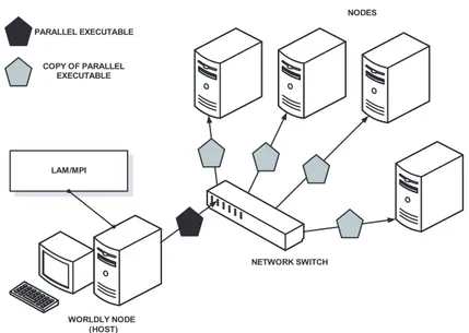
After we get a parallel executable, we run our parallel program with the aid of LAM/MPI. LAM/MPI supports SPMD approach and it actually sends the parallel executable, which is compiled on host, to all other nodes. Then, when program execution starts, each processor does the task that is predefined for itself in this single executable code:
During the installation and especially in usage of the parallel libraries and interfaces, we have faced some problems. This situation occurs occasionally; because, we work on the cutting edge in the scientific problem solving. Thus we are the firsts to face these new problems in our country. Especially, the problems that we experienced are mainly based on the compatibility problems between parallel libraries, such as PETSc and Scalable LAPACK (ScaLAPACK)—parallel version of LAPACK—, and parallel implementations, LAM/MPI in our case. In spite of these problems, we worked continuously and have achieved a stable parallel software environment which give us the chance to improve and run our
NODES WORLDLY NODE (HOST) NETWORK SWITCH PARALLEL EXECUTABLE COPY OF PARALLEL EXECUTABLE LAM/MPI
Figure 2.4: Run of a parallel program on homogenous Beowulf cluster parallel programs.
2.2
Hybrid 32-Bit Intel Pentium IV and 64-Bit
Intel Itanium II Cluster
While beginning our parallel programming approach, we assumed that we might assign some of the hard tasks of the parallel program on a special node of the cluster, which has more computational power and memory capacity. For this purpose, we decided to connect our newly bought multiprocessor system, which is based on 64-Bit Intel Itanium II processor architecture, to our homogeneous 32-Bit Intel Pentium IV cluster. This new multiprocessor system has two 64-Bit Intel Itanium II processors, which operates at 1.5 GHz and 24 GBytes of memory. Therefore, as it is mentioned before, this huge memory capacity and computational power might be successfully used in a master-slave approach in our continuous program development effort.
64-bit architecture of Intel Itanium is completely different from the normal 32-bit Intel Pentium based processors. As a result, assembly instruction set of this
new processor also differs from the instruction set of 32-Bit Intel Pentium based processors; so, Itanium multiprocessors need its own executable which is compiled specially for its instruction set. Thankfully, Intel company developed a special version of compilers which we used for generating the executable for our 32-bit machines; Intel Fortran and C/C++ compilers for the Itanium architecture are freely available for Linux operating environment and we installed those mentioned compilers on our multiprocessors system.
Difference between the architectures of processors that we deployed in our cluster system shifts our programming strategy to MPMD programming tech-nique:
32-BIT NODES
64-BIT WORLDLY NODE (MAIN HOST)
PARALLEL EXECUTABLE FOR 32-BIT PROCESSOR COPY OF PARALLEL
EXECUTABLE FOR 32-BIT PROCESSOR
LAM/MPI COMPILED FOR 64-BIT PROCESSOR
PARALLEL EXECUTABLE FOR 64-BIT PROCESSOR
32-BIT SLAVE HOST
LAM/MPI COMPILED FOR 32-BIT PROCESSOR
NETWORK SWITCH
Figure 2.5: Execution of a parallel program on hybrid Beowulf cluster As it can be seen in Fig. 2.5, we generate two different executables from the same parallel MLFMA code for two different processor architectures. We build the executable for Itanium machine on itself. On the other hand, we specially allocate one 32-bit node of parallel cluster in order to compile programs and to store parallel and sequential system tools for the rest of the 32-bit nodes. De-pending on this methodology, parallel executables for 32-Bit nodes are generated on the mentioned special 32-bit node of the cluster, which can be named as a slave host—shown in Fig. 2.5.
64-bit machine and users’ homes are mounted by the nodes from these multi-processors. Nevertheless, as explained before, 32-bit machines need some system programs, which are compiled for their architecture and these system programs are stored on the 32-bit slave host. Other nodes of the cluster mount these system programs, which are compatible for 32-bit systems from this special node. All those mounting operations are done with the aid of NFS.
64-BIT MAIN HOST 32-BIT SLAVE HOST
NODE 1 NODE N
LIBRARIES COMPILERS PARALLEL APPLICATIONS
FOR 64-BIT PROCESSOR
HOME DIRECTORIES HOME DIRECTORIES HOME DIRECTORIES HOME DIRECTORIES LIBRARIES COMPILERS PARALLEL APPLICATIONS
FOR 32-BIT PROCESSOR
LIBRARIES COMPILERS PARALLEL APPLICATIONS
FOR 32-BIT PROCESSOR
LIBRARIES COMPILERS PARALLEL APPLICATIONS
FOR 32-BIT PROCESSOR HOME MOUNTING SYSTEM PROGRAMS MOUNTING NODES
Figure 2.6: Mountings in the hybrid cluster
In the software topology, as depicted in Fig. 2.6, there are a lot of mounting operations done between computers. Since all these mountings use the network of the cluster, the system’s overall network performance degrades. In addition, compiling different programs on different architectures and servers working on host computers, decrease the performance of the hosts. Moreover, as we continue to improve our parallel code, we experience that we do not need such a special computer for the tasks of our program. Therefore, we took out our 64-Bit Ita-nium multiprocessors from the cluster and returned to our homogeneous Beowulf architecture.
2.3
Proposed 64-Bit AMD Opteron Cluster
In the beginning of 2004, Advanced Micro Devices (AMD) released the new 64-bit processors for personal usage and computational purposes. These new processors support both 64-bit and 32-bit assembly instruction sets; therefore, AMD’s pro-cessors give a very huge flexibility in many applications. In addition to this flexibility, Linux operating system developers always have sympathy for AMD processors; because Intel generally supports and advices to use Microsoft’s oper-ating system products on its products—Microsoft has been the natural rival of Linux since the beginning of Linux’s first release. As a result, Linux developers released 64-Bit Linux operating systems for these new processors in a very short amount of time; so, AMD’s cheap and powerful new processors serve as a good choice for Beowulf cluster computing solutions.
AMD produces many different versions of these new processors, but the most interesting and suitable processor for scientific computing is its Opteron archi-tecture. AMD Opteron is specially designed for server applications and heavy scientific computing. It comes in three different models 1-way, 2-way and 8-way. 1-way model can only be used on single processor mainboards, 2-way can be used on single processor and double processors systems and 8-way can be used in a system which can support 8 AMD Opteron processors. In Turkey, only the 2-way version is sold. We obtained many positive feedbacks about this architecture and decided to build one such Opteron based system and compare its performance with the other computers that we have. Thus, we would be able to plan how to build our future cluster systems and decide which hardware components should be chosen in order to get optimum performance in our parallel program develop-ment efforts. For this purpose, we bought a 2-way AMD Opteron multiprocessors system, whose processors operate at 1.8 GHz, and 4 GBytes of memory installed in it. The system has a NUMA communication architecture; 2 GBytes of RAM is directly addressed by one processor and the remaining 2 Gbytes of memory is addressed by the other processor. Thus, when a sequential application needs memory greater than 2 GBytes, its execution speed decreases a little bit because of this NUMA architecture.
After buying this new system, we used the sequential version of MLFMA program as a benchmark tool and we compared performance of the computer systems in different parts of the sequential MLFMA program. The following hardware architectures are compared:
• Intel Prescott Pentium IV, 2.8 GHz single processor computer with 2 GBytes of memory
• AMD Opteron 244, 1.8 GHz dual multiprocessors computer with 4 GBytes of memory
• Intel Itanium II, 1.5 GHz dual multiprocessors computer with 24 GBytes of memory
In order to compare AMD Opteron multiprocessors with the other systems that we have, we especially focused on the performances of these machines in the two important parts of MLFMA: nearfield matrix Znearfilling module and
matrix-vector multiplication module in iterative conjugate gradient stabilized (CGS) solver. These performance plots are given in Fig. 2.7 and Fig. 2.8, respectively:
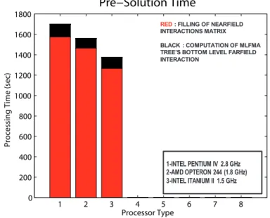
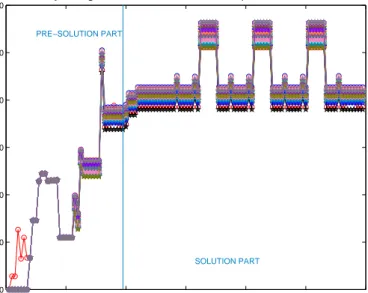
1 2 3 4 5 6 7 8 0 200 400 600 800 1000 1200 1400 1600 1800 Processor Type Proc essi ng T ime (s ec) Pre−Solution Time 1-INTEL PENTIUM IV 2.8 GHz 2-AMD OPTERON 244 (1.8 GHz) 3-INTEL ITANIUM II 1.5 GHz
RED: FILLING OF NEARFIELD INTERACTIONS MATRIX
BLACK : COMPUTATION OF MLFMA TREE’S BOTTOM LEVEL FARFIELD INTERACTION
Figure 2.7: Performance comparison of different processors with pre-solution part of sequential MLFMA
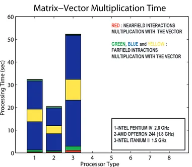
1 2 3 4 5 6 7 8 0 10 20 30 40 50 60 Processor Type Proc essi ng T ime (sec)
Matrix−Vector Multiplication Time
1-INTEL PENTIUM IV 2.8 GHz 2-AMD OPTERON 244 (1.8 GHz) 3-INTEL ITANIUM II 1.5 GHz
RED : NEARFIELD INTERACTIONS MULTIPLICATION WITH THE VECTOR GREEN, BLUE and YELLOW: FARFIELD INTRACTIONS MULTIPLICATION WITH THE VECTOR
Figure 2.8: Performance comparison of different processors with matrix-vector multiplication in the iterative solver part of sequential MLFMA
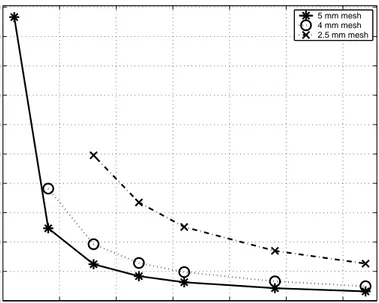
These benchmark plots are obtained for the scattering solution of sphere at 6 GHz and this problem corresponds to the solution of a 132003 unknown full dense matrix. As can be seen from the first plot, Fig. 2.7, nearfield matrix filling performance of Itanium machine is the best; despite this, in the matrix-vector multiplications, AMD Opteron machine gives the best timing results. Ac-tually, matrix-vector performance of machines is more important with respect to nearfield matrix filling operation; because, this multiplication is done many times in the iterative solution part of both sequential and parallel MLFMA. Moreover, as the problem size grows—number of unknowns increase, iteration numbers also increase, whereas only one nearfield matrix filling operation is done for the same problem. Therefore, if we want to solve larger problems, we have to choose a processor which performs better with respect to others in matrix-vector multipli-cations. As a result, we choose AMD Opteron dual multiprocessors as the nodes of our proposed cluster, which is going to be built in shortly.
2.4
ULAKBIM Cluster
Our cluster at Bilkent consists of four nodes. Despite this small cluster, our paral-lel program has been improved a lot by our group since 2002. In this improvement process, main goal is to build a parallel program which is scalable. For this reason, we wanted to test our program on a bigger cluster which has more processors. Fortunately, TUBITAK built a high performance cluster at ULAKBIM which has 128 nodes and we obtained access to this system and the system administrators of this cluster cooperated with us for our scalability measurements.
This cluster at ULAKBIM has 128 single processor machines which have Intel Celeron Pentium IV processor operating at 2.6 GHz and 1 GBytes of memory installed on all machines. We did certain parallel profiling measurements on those machines and from these measurements, we observed that the network speed of the cluster is more faster than ours. Since, we plan to build a new parallel computer and we had to make decisions on hardware components of this proposed cluster, we used our parallel program as a profiling tool in order to test and compare the speed of network connection at ULAKBIM’s cluster, on our cluster and on the two processors of dual AMD Opteron multiprocessors. To achieve this aim, we did measurements on two processors of ULAKBIM’s cluster and our cluster. In addition to that, we measured the two processor AMD Opteron by using our parallel MLFMA program. In Figs. 2.9-2.10, these benchmarking results are plotted:
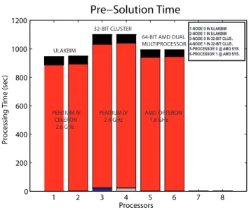
1 2 3 4 5 6 7 8 0 200 400 600 800 1000 1200 Processors Proc essi ng T ime (sec) Pre−Solution Time ULAKBIM 32-BIT CLUSTER
64-BIT AMD DUAL MULTIPROCESSOR PENTIUM IV CELERON 2.6 GHz PENTIUM IV 2.4 GHz AMD OPTERON 1.8 GHz 1-NODE 0 IN ULAKBIM 2-NODE 1 IN ULAKBIM 3-NODE 0 IN 32-BIT CLUS . 4-NODE 1 IN 32-BIT CLUS . 5-PROCESSOR 0 @ AMD SYS. 6-PROCESSOR 1 @ AMD SYS.
Figure 2.9: Performance comparison of different processors with pre-solution part of parallel MLFMA 1 2 3 4 5 6 7 8 0 2 4 6 8 10 12 14 16 18 Processors Proc essi ng T ime (sec)
Matrix−Vector Multiplication Time
ULAKBIM
32-BIT CLUSTER
64-BIT AMD DUAL MULTIPROCESSOR
1-NODE 0 IN ULAKBIM 2-NODE 1 IN ULAKBIM 3-NODE 0 IN 32-BIT CLUS . 4-NODE 1 IN 32-BIT CLUS . 5-PROCESSOR 0 @ AMD SYS. 6-PROCESSOR 1 @ AMD SYS.
Figure 2.10: Performance comparison of different processors with matrix-vector multiplication in the iterative solver part of parallel MLFMA
From the figures, it can be easily observed that the performance of dual AMD multiprocessors is the best for matrix-vector multiplications. The red and gray parts on Fig. 2.10 actually shows the communications between processors in matrix-vector multiplications—red corresponds to the sending and receiving electromagnetic data, mainly translations; gray denotes idle time. As you can see from the graph, network performance of ULAKBIM is much better than our cluster’s network connectivity, but it is still not as good as our AMD Opteron system. We expected this situation before we did our measurements; because AMD Opteron processors do their communication on the same motherboard; no network interface is used during these communications. On the other hand, in our cluster and at ULAKBIM, processors communicate through an ethernet based network. Actually ULAKBIM has a really fast ethernet system since they use gigabit ethernet interfaces and network switches in order to connect their com-puters. In spite of having a 100 Mbit/sec fast ethernet connection, here in our lab, it is ten times slower than ULAKBIM’s gigabit connection. Depending on these measurements, we plan to use a gigabit network or a much faster network in our future cluster.
Parallelization of MLFMA
3.1
Adaptation of MLFMA into Parallel System
Before starting to parallelize our MLFMA code, firstly, we tried to adapt and run the original sequential version of the program on our message-passing multicom-puter system. Our original program is written in DIGITAL FORTRAN 77, which supports Cray pointers for the sake of dynamic memory allocation (DMA). These dynamically allocated memory structures increase the efficiency of memory usage. Nevertheless, the default FORTRAN 77 compiler, g77, in Linux systems does not support this feature; therefore, we could not compile the sequential MLFMA code directly and we could not run it on our Linux based parallel computer system.
For the solution of this problem, we primarily focused on the usage of open source software solutions and compilers, which are installed as default features in Linux based operating systems; we realized that open source Fortran and C/C++ compilers, g77 [15] and gcc, are compatible with each other and Fortran programs are able to call functions or features of C/C++ language by the aid of this compatibility. Then, we wrote small C subroutines which implements malloc (memory allocation) feature of this language and used them in Fortran trial programs. These trials were successful, and then we used these C subroutine in our sequential MLFMA code and it worked well. In spite of all these successful
trials, this new feature of C certainly complicates the array structure of our program. In addition, it also complicates the readability of our program. As a result of these facts, we started to look for another solution for this compilation problem.
At this point, we found freely available Intel Linux FORTRAN compiler, which supports many extensions in Fortran semantics and has a backward compatibility with the old FORTRAN distributions. We installed this free compiler in our sys-tem and compiled our parallel applications, such as MPI and parallel-sequential libraries, with that compiler. We followed that way, because we do not want to face any compatibility problems because of different compilations of these system programs. After all these, we compiled the sequential version of MLFMA suc-cessfully and executed it on a single node of the parallel cluster. Then, we put this sequential version of MLFMA as a single parallel process in a simple parallel program and executed it as such and we realized that we could start to parallelize our code. Following chapters are going to give the details of this parallelization process.
3.2
Partitioning Techniques
Message-passing parallelization paradigm is actually based on partitioning of data structures among processors. Most of the time, processes do similar tasks on those partitioned data and depending on the type of the problem or computation, they interchange their partitioned or processed data. These partitioned data structures are generally arrays or array-based data structures. One-dimensional arrays and two dimensional arrays are the most commonly used array architectures. For the sake of parallelization, these array structures are firstly partitioned; then, these partitions are mapped onto the processors depending on the criteria of the parallelization approach e.g., minimizing communication, equalizing memory usage, and etc. Arrays can be partitioned as shown in Fig. 3.1:
(a) (b) COLUMN-WISE
DISTRIBUTION
ROW-WISE DISTRIBUTION 4 x 6 GRID
2 x 6 GRID
Figure 3.1: (a) One-dimensional partitioning of an array (b) two-dimensional partitioning of an array
In Fig. 3.1, common array partitioning methodologies are shown. These par-titioned arrays can be distributed among the processor statically or dynamically, depending on the application or problem. We used statical mapping of these ar-rays on our processors, because, we know the sizes of the arar-rays that we need for our electromagnetic data and we try to minimize the communication over proces-sors. For these reasons, in our program, array load of each cluster is determined in the beginning of the code.
In our MLFMA code, all arrays related with the matrix information of our problem, Znear and Zfar matrices, which need a lot of memory in order to be
stored, are one-dimensional arrays. Therefore , partitioning of these arrays among processors is not trivial; because of that reason, we started our parallelization efforts from the relatively easily parallelized parts of our program.
3.3
Partitioning in Parallel MLFMA
We mentioned that our strategy for the parallelization of MLFMA code is to parallelize relatively simple parts at the beginning; then, we decided to move on to more complex parts of the program. According to our point of view, the first parallelized part of MLFMA is the filling of preconditioner matrix [16], which is used in the iterative CGS solver part of the program. After parallelization of this part, we realized that the partitioning applied on the data structure of preconditioner can be used to partition the whole tree structure of MLFMA among the processors.
3.3.1
Partitioning of Block Diagonal Preconditioner
In the iterative solution techniques, preconditioners are used in order to get a better solvable matrix equation system. Preconditioners are actually matrices, which are very similar to the inverse of the original matrix. In our MLFMA code, the preconditioner, M, is extracted from the near-field matrix, Znear, of
our matrix system and then it is applied to the matrix system:
M−1
.Z.x = M−1
.y (3.1)
where x and y are the unknown and excitation vectors, respectively.
As stated before, M is extracted from Znear. Actually, M contains the most
powerful terms of Znear matrix, which are the self interaction terms of the
in-duced electromagnetic currents grouped in the last level clusters of MLFMA tree structure—self interactions refer to the near-field interactions of clusters in Znear
with themselves. These interaction terms are placed as blocks in the diagonal of near-field matrix; because of this placement, the preconditioner is named as block diagonal preconditioner (BDP). In order to build our preconditioner, we take out these blocks and treat each of them as a normal matrix system: LU fac-torization is applied on each of these blocks and the inverses of them are taken. LAPACK subroutines, ZGETRF and ZGETRI [17] are used in these operations,
respectively. Finally inverses of these blocks are written in the memory in order to built the preconditioner matrix:
NEARFIELD MATRIX SELF INTERACTIONS OF A CLUSTER LAPACK SUBROUTINES MATRIX BLOCK INVERSE MATRIX BLOCK PRECONDITIONER MATRIX
Figure 3.2: Extraction of preconditioner matrix
In parallelization, each of these clusters’ self interaction blocks are partitioned among processors, equally; so, each of the processor gets equal number of blocks according to this partitioning. For this purpose near-field matrix’s corresponding blocks are row-wise partitioned and then partitioned blocks are assigned to a processor consecutively as it is shown in Fig. 3.3:
PROCESSOR 0
PROCESSOR M M+1 PROCESSORS
LAST LEVEL CLUSTERS’ SELF INTERACTIONS
3.3.2
Partitioning of MLFMA Tree Structure
It is stated before that MLFMA is actually based on the grouping of electromag-netic interactions in clusters and those clusters are re-grouped in bigger clusters recursively. As a result, we get a tree structure. In that tree structure, bigger clusters have direct electromagnetic relations with the small clusters, which are in its group. For that reason, a cluster, which contains a small cluster, is called as parent of that cluster and the small cluster is called as child of the bigger cluster. Thus, MLFMA’s far-field operations—aggregations, disaggregations and translations [11]— and near-field matrix filling operations are done on this hier-archical tree structure. Actually the near-field matrix, Znear, is computed by last
level cluster’s electromagnetic interactions; because in order to compute the near-field matrix, we should interact each discretized induced electromagnetic current with its near-field neighbor directly according to the MoM. Hence near-field in-teractions are calculated depending on this approach, we do not need to do any computation for near-field interactions of the upper levels clusters in MLFMA tree.
In the parallelization of BDP, last level clusters of the MLFMA tree are parti-tioned among the processors in order to assign equal number of last level clusters in each of the processors. Partitioning of MLFMA is based on this basic par-titioning: We simply start to put last level clusters’ parents on the processor where their children are deployed, and this strategy is applied from the last level, bottom level of clusters, to the top level. This situation is depicted in Fig. 3.4:
C0 C1 C3 C4 C5 C6 C7 C8 PR1 COPY OF PR2 PR2 PROCESSOR 1 PROCESSOR 0 LAST LEVEL CLUSTERS UPPER LEVELS OF MLFMA TREE PR : PARENT CLUSTER C : CHILD CLUSTER