368 IEEE TRANSACTIONS ON COMPUTER-AIDED DESIGN OF INTEGRATED CIRCUITS AND SYSTEMS, VOL. 15, NO. 3, MARCH 1996
ered in the paper, signal probability based transistor reordering is also valid in CMOS dynamic logic, where considerable power dissipation occurs in the internal nodes of dynamic gates. Furthermore, since velocity saturation effects are expected to increase the maximum number of MOSFET’s that can be serially connected in smaller geometries [l], this techniques will remain valid with scaled device sizes.
The principal advantage with the proposed approach is that it does not increase the number of transistors or require any architectural modifications in the design. Transistor reordering also does not alter the global routing of the circuit as all changes are local. The timing characteristics of the design may, however, be altered by the reordering scheme. This may limit the applicability of the technique in some gates along the critical paths. Transistor reordering based reductions in power dissipation are applicable across CMOS circuits and with appropriate tools support can be incorporated in both custom and ASIC design methodologies.
A New Method for Nonlinear Circuit
Simulation in Time Domain: NOWE
Ogan Ocali, Mehmet A. Tan, and Abdullah AtalarAbstract- A new method for the time-domain solution of general nonlinear dynamic circuits is presented. In this method, the solutions of the state variables are computed by using their time derivatives up to
some order at the initial time instant. The computation of the higher order derivatiws b equivalent to solving the same linear circuit for various sets of dc excitations. Once the time derivatives of the state variables are obtained, an approximation to the solution can be found as a polynomial rational function of time. The time derivatives of the approximation at the initial time instant are matched to those of the exact solution. This method is promising in terms of execution speed, since it can achieve the same accuracy as the trapezoidal approximation with much smaller number of matrix inversions.
I. INTRODUCTION
As VLSI technology improves, circuit simulators face the challenge of increasing circuit complexity. Therefore, it seems the need for the faster algorithms will never come to an end. The numerical integration approximations such as Forward Euler, Backward Euler, Trapezoidal ApproKimations [ 11, and Asymptotic Waveform Eval- uation (AWE) [Z] are the prominent methods for the time-domain ACKNOWLEDGMENT
The authors wish to thank the members of the VLSI &roup at the University of Rochester and the anonymous reviewers for their valuable comments. The suggestions of B. Cherkauer and Anonymous Reviewer 1 were especially incisive.
REFERENCES
T. Sakurai and A. R. Newton, “Delay analysis of series-connected MOSFET circuits,” IEEE J. Solid-State Circuits, vol. 26, pp. 122-131, Feb. 1991.
B. S. Cherkauer and E. G. Friedman, “Channel width tapering of serially connected MOSFET’s with emphasis on power dissipation,” IEEE Trans. VLSI Syst., vol. 2, pp. 100-1 14, Mar. 1994.
K. Roy and S. Prasad, “SYCLOP: Synthesis of CMOS logic for low power applications,” I992 IEEE Int. Con$ Computer Design, Oct. 1992, pp. 464-467.
A. Shen, A. Ghosh, S. Devadas, and K. Keutzer, “On average power dissipation and random testability of CMOS combinational logic net- works,” 1992 IEEE/ACM Int. Con5 Computer-Aided Design, Nov. 1993, pp. 402406.
B. S. Carlson and C. Y. Roger Chen, “Performance enhancement of CMOS VLSI circuits by transistor reordering,” 30fh ACMLEEE Design Automation Con$, June 1993, pp. 361-366.
F. N. Najm, R. Burch, P. Pang, and I. N. Hajj, “Probabilistic simulation for reliability analysis of CMOS VLSI circuits,” IEEE Trans. Computer- Aided Design, vol. 9, pp. 439450, Apr. 1990.
M. A. Cirit, “Estimating dynamic power consumption of CMOS circuits,” IEEE Int. Con$ Computer-Aided Design, Nov. 1987, pp. 5 34-5 37.
B. Johnson, T. Quarles, A. R. Newton, D. 0. Pederson, and A. Sangiovanni-Vincentelli, “SPICE3 Version 3D2 User’s Manual,” Dept. Elec. Eng. Comput. Sci., University of California, Berkeley, 1990. R. Marculescu, D. Marculescu, and M. Pedram, “Switching activity analysis considering spatio temporal correlations,” 1994 IEEE/ACM Inf. Con$ Computer-Aided Design, San Jose, CA., Nov. 1994, pp. 294-299. N. H. E. Weste and K. Eshraghian, Principles of CMOS VLSI Design 2nd ed. Reading, MA: Addison-Wesley, 1993.
analysis of electronic circuits. There also exist some exponential fitting algorithms such as those implemented in the programs MOTIS
[3], [4] and CINNAMON [5] and XPSim [6] which are tailored for
the MOS circuits only. These methods provide varying accuracyhme- complexity tradeoffs. The trapezoidal integration is used in SPICE [7] and preferred in many cases because .of both stability and accuracy
[&I.
However, in the time domain analysis of a nonlinear circuit, the Trapezoidal Approximation at every time step requires a new Newton-Raphson iteration. Furthermore, each Newton-Raphson iteration step involves the solution of a new linear resistive circuit, which requires an LU decomposition [I] and a forward and back substitution (FBS). AWE has proven itself to be a very fast and an accurate alternative for time domain analysis of linear dynamic circuits. The power of AWE comes from the fact that it performs a single LU decomposition and a few FBS’s for the entire time region for which the transient analysis is performed. The analysis with AWE is concluded by a simple evaluation of the linear combination of exponential terms. The speed and precision of the AWE method is employed in piecewise-linear AWE (PLAWE) [9], by using piecewise linear models for nonlinear elements. In the PLAWE approach, a slowdown may result when the number of segments of the models is increased to improve the accuracy.Inspired by the AWE approach, we propose a Nonlinear circuit Waveform Evaluation (NOWE) method for the transient analysis of ‘nonlinear circuits. NOWE is based on the waveform approximation of the solution. The approximate waveform i s evaluated as the sum of polynomial rational function of time whose time derivatives Manuscript received July 21, 1992; revised March. 1, 1994, July 26, 1994, and December 5, 1995. This work was supported in part by the Scientific and Technical Research Council of Turkey Project EEEAG-24. This paper was recommended by Associate Editor J. White.
0. Ocall and A. Atalar are with the Department of Electrical and Electronics Engineering, Bilkent University, Ankara, Turkey.
M. A. Tan was with Bilkent University, Ankara, Turkey. He is ’now with Silicon Systems Inc., a TDK Group Company, Tustin, CA 92680 USA.
Publisher Item Identifier S 0278-0070(96)01844-1.
IEEE TRANSACTIONS ON COMPUTER-AIDED DESIGN OF INTEGRATED CIRCUITS AND SYSTEMS, VOL. 15, NO. 3, MARCH 1996 369
match the time derivatives of the exact solution. Computation of all time derivatives of the exact solution requires only one LU decomposition as in AWE. Once the LU factorization has been completed, performing one FBS per derivative order is sufficient. The approximate solution is valid for a longer interval of time than the one achieved in Trapezoidal Approximation.
The next section explains the proposed approach and its imple- mentation. The performance of this method is verified through two examples in Section I11 and compared with SPICE in terms of the time complexity and accuracy.
11.
THE
METHOD: NOWEAssume that we are given a circuit which consists of one-port and two-port elements, namely resistors, capacitors, inductors, and independentkontrolled sources, all of which may be linear or non- linear. Also, assume that at time t = O+ we know the initial values of voltages of capacitors, currents of inductors, and the controlling parameters of nonlinear controlled sources. NOWE basically attempts to find a waveform whose time derivatives up to a certain order match to the time derivatives of the exact solution of the considered variable. First of all, we shall explain how to find a polynomial rational function of time whose time derivatives match the time derivatives of the exact solution of a variable (i.e., voltage or current) under consideration. Polynomial rational function is chosen instead of sum of complex exponentials because it requires the solution of only a set of linear equations rather than a polynomial equation. Moreover, there is no particular reason to choose exponentials, since the circuit is nonlinear. At the end of this section, the computation of the time derivatives of the exact solution will be described.
2.1 Finding the Polynomial Rational Function in the Time Domain Let d i ) , i = 0 , 1 , 2 , . . . , 2 q denote the ith derivative of ~ ( t ) ,
which is the exact solution of any variable of the circuit, evaluated at t = O+. Assume that
where ? ( t ) is an approximation to the exact solution ~ ( t ) , and N ( t ) and D ( t ) are the finite degree numerator and denominator polynomials of time, respectively, that is
Assume that R ( t ) can be expressed as
m
(3) (4)
( 5 ) i=O
The task is to find ni's and d i ' s such that
Note that
d k ) ' s ,
in other words, rk's can be computed from the circuit given, as shall be explained later on. Having known Tk's, the coefficients nz's and d,'s should satisfy(7)
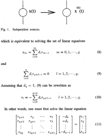
Fig. 1. Independent sources.
which is -equivalent to solving the set of linear equations
m
and
Assuming that dq = 1, (9) can be rewritten as
In other words, one must first solve the linear equation
(9)
for d z ' s . Afterwards, n,'s are computed from (8). An efficient
algorithm for the solution of (1 1) is available at the complexity of
O ( q 2 ) instead of O ( q 3 ) [lo].
2.2 Evaluating Derivatives
We will show that the task of finding the time derivatives of any voltage or current in the given circuit is equivalent to solving the same linear resistive circuit for various appropriate independent currentlvoltage sources.
First of all, let us recognize the fact that Kirchhoff s Current Law (KCL) and Kirchhoffs Voltage Law (KVL) hold for all orders of derivatives of currents and voltages in the circuit. That is
(12) d" dtn KCL: A i ( t ) = 0 A - i ( t ) = 0 KVL: v - A T e ( t ) = 0 -v d" - A T c e ( t ) = 0 (13) dt" dt"
for n = 0 , 1 , 2 , .
. .
,
where A is the reduced incidence matrix, edenotes the node voltages, v ( t ) and i ( t ) stand for branch voltages and currents. We can now consider the nth time derivatives as new branch variables, i.e., the voltages and currents of a circuit (let us refer to it as the nth derivative circuit) in the same topology and with possibly new branch constitutive relations. Next, we shall investigate the branch constitutive relations of the nth derivative circuit for various types of elements.
2.2.1 Independent Sources: Obviously, an independent source is replaced by the same type of independent source in the nth derivative circuit whose value is equal to the nth time derivative at t = 0 of the original independent source. The simulation is valid within the time intervals where the time derivatives exist and are continuous. The entire NOWE must be repeated at the discontinuity borders.
370 IEEE TRANSACTIONS ON COMPUTER-AIDED DESIGN OF LNTEGRATED CIRCUITS AND SYSTEMS, VOL. 15, NO. 3, MARCH 1996
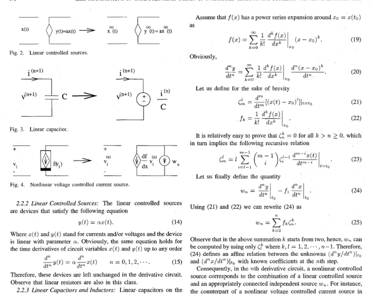
Fig. 2. Linear controlled sources.
i
(n+l)Fig. 3 . Linear capacitor.
+
n
Fig. 4. Nonlinear voltage controlled current source.
2.2.2 Linear Controlled Sources: The linear controlled sources are devices that satisfy the following equation
y(t) = a!z(t). (34)
Where z( t ) and y ( t ) stand for currents and/or voltages and the device is linear with parameter a. Obviously, the same equation holds for the time derivatives of circuit variables z ( t ) and y(t) up to any order (15) Therefore, these devices are left unchanged in the derivative circuit. Observe that linear resistors are also in this class.
2.2.3 Linear Capacitors and Inductors: Linear capacitors on the circuit obey the following differential equation
d" d"
dt" dt"
- y ( t ) = a!-x(t) n = 0 , 1 , 2 , .
.
..
(16) By taking the nth derivative of (16) with respect to t , one can obtain
Cd,,,vc(t) = --zc(t) n = 0 , 1 . 2
:...
(17) As can be observed from (17), (n+
1)st derivative of the voltage is independent of ( n+
1)th derivative of the current. The ( n+
1)st derivative of the voltage only depends on the nth order derivative of the current. Therefore, in the (n+
1 ) s t derivative circuit, linear capacitors are replaced by independent voltage sources of value (l/C)(d"/dt")r.(t) evaluated at time t = O+. By the duality principle [ll], in the (n+
1)st derivative circuit, every Linear inductor is replaced by an independent current source of value (l/L)(d"/dt")vL(t) evaluated at time t = O+ where L is the inductance.2.2.4 Nonlinear Controlled Source: Assume that a nonlinear con- trolled source is defined by
d at C - v c ( t ) = ic(t). d"+l d" . at"
d t )
= f ( x ( t ) ) (18)where z( t ) and y ( t ) stand for the controlling and controlled variables (i.e., voltage or current) of the element, respectively. We also assume f (.) is n times differentiable. This assumption may require that the time domain analysis be performed in appropriate intervals if the nonlinearity is given as piecewise analytic functions.
Assume that f(z) has a power series expansion around xo = z ( t 0 )
as
Obviously,
Let us define for the sake of brevity
It is relatively easy to prove that
&
= 0 for all k>
n2
0, which in turn implies the following recursive relationLet us finally define the quantity
Using (21) and (22) we can rewrite (24) as wn = f k d .
k=2
Observe that in the above summation k starts from two, hence, w, can be computed by using only
Cf
where k , 1 = 1 , 2 ,. . .
,
n- 1 . Therefore, (24) defines an affine relation between the unknowns ( d " y / d t " ) l t ,and ( d " z / d t " ) l t o with known coefficients at the nth step. Consequently, in the nth derivative circuit, a nonlinear controlled source corresponds to the combination of a linear controlled source and an appropriately connected independent source w,
.
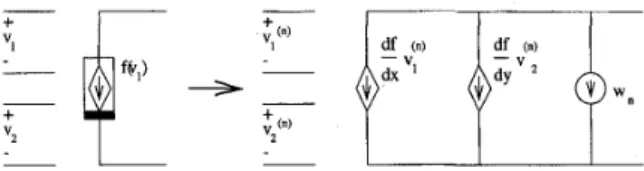
For instance, the counterpart of a nonlinear voltage controlled current source in the nth derivative circuit is a linear voltage controlled current source with an independent current source W, connected to its output portin parallel, as shown in Fig. 4.
For the first derivative circuit, we set W I = 0. The solution of
this circuit provides the first order derivatives of the circuit variables, enabling us to set the initial value of the recursion
c : = -
.
2
lto
At the nth step, we compute
<,",
k = 2 , .. . ,
n using (23) and store them. Afterwards, we compute W, from (25) and use this value to setup the nth order derivative circuit equations. By using the solution of this circuit we set
d " z =
=Ito
which completes the computation of the nth derivatives of the circuit variables.
Note that although the derivation of the recursion presented above is valid for any analytic nonlinearity, the computational burden at the nth step is not very high (e.g., at O ( n 2 ) for each nonlinear controlled source, where n is the derivative order). Furthermore, wn can be computed even more efficiently in case of the most encountered functions such as exponentials in the model of semiconductor diodes and bipolar junction transistors or square-law functions in the model of MOSFET's.
IEEE TRANSACTIONS ON COMPUTER-AIDED DESIGN OF INTEGRATED CIRCUITS AND SYSTEMS, VOL. 15, NO. 3, MARCH 1996 371
ranging from two to n. We use (36) and (37) to obtain a;, b;, and I ranging from two to n f r o m a F , b t i , k = l , . . . , n - 1, not using ( d " z / d t " ) , ( d " y / d t " ) . Therefore (38) defines an affine coefficients. This relation implies that the corresponding element to a circuit is an appropriate combination of two linear controlled sources and an independent source. For instance, the counterpart of a non- -
~
+ relation among ( d " z / d t " ) , ( d n y / d t " ) , and ( d " z / d t " ) with known controlled source with two controlling variables in the nth derivative
-0'
"1
+
i"
\Fn
"2
;p
~ ~
Fig. 5. Nonlinear voltage controlled current source two controlling voltages.
linear voltage controlled current source with two controlling voltages in the nth derivative circuit is two linear voltage controlled current Sources whose output ports are connected in parallel together with an independent current source, as shown in Fig. 5. Finally we can sumarize the task at the nth derivative computation for a doubly controlled source as follows.
First compute a:, b k , k , I = 2 , .
. ,
n using (36) and (37), and store This derivation is slightly different in the case of controlledsources that are controlled by two Controlling variables as in of MOSFET's and BJT's.
defined by
Let us consider a controlled source with two controlling variables
(28)
4 t )
= f(z(t),dt))
them since they will be needed in the forthcoming steps. Then, find
& l , 2
5
where z ( t ) and y ( t ) are the controlling and ~ ( t ) is the controlled
variable. resnectivelv. + 1
5
though(33). Next find wn as
We assume a bivariate power series expansion of
f
(z, y ) around W n = f k 1 4 E 1 . (39)k , l > O 2 < k + l < n
the operating point ( z ( t o ) , y ( t 0 ) ) as
Use w n to set up the circuit equations. Finally, use the solution of
k=O l=O " 0 , Y O the circuit to set
' (z
-
z O p ( Y-
Y 0 ) l (29) where 20 = z ( t 0 ) and yo = y(t0). Consequently, we have1 d " z an = - dt" A n b: = ? (41) d t n m o o completing step n.
Practically, for small to moderate n (10 N 14) the computational
complexity of the recursion described above can be tolerated. More-
k l d" (31) over, the amount of computation can be drastically reduced for certain
analytical functions that do not require a power series expansion. 2.2.5 Nonlinear Capacitor: We assume that a nonlinear voltage controlled capacitance is defined by
(30) d"
dt"
-f(.(t),
d t ) )
= f k l & l k=O 1=0 where, in parallel to the singly controlled sourcedt"
4 n
= - ~ O ) ' ( Y - ~ 0 ) ' I I t o(32)
Observing that ( d " / d t " ) [ z ( t ) - z O ] k l t o = 0 if IC
>
n we can show q ( t ) = f ( v ( t ) ) (42) thatn-1 where q is the charge on the capacitor. Taking derivatives with respect
to tn times and recalling the fact that the current through the capacitor i = d q / d t we obtain
4;'
= ( y ) a F b k - t (33) t=k where and d i ( t ) d Z q ( t ) - df d 2 v ( t ) d 2 f d v ( t ) d 2 v ( t ) -=--.-- (35) d t d t 2 d v d t 2 +-(TI
*
dt2
d2 - dtc k - 1 - d t d v 2(
d t)
b1 - - [ y ( t > - .olEltowhich can be computed recursively as d i ( t ) _ _ - - d 2 f d v ( t )
~ (44) - (45) k - 1 d " - l i ( t ) d " v ( t ) - d t n - 1 bf = k ( k ' ) b ; - ' ~ ( ' - ~ ) . (37) - - 3 ~ 2 - 1
($)
dt" Finally, we define d" d" d" wn = - - . ( t ) d t n - f l o - z ( t ) dt" - f01 - ~ ( t ) I t o dt" k+l<n k,l=Owhere un depends only on time derivatives of capacitor voltage up to the order n - 1 and ( d k / d v k ) f ( v ) k = 2 , 3 , .
. .
,
n. So, we replace nonlinear capacitors with independent voltage sources in series as shown in Fig. 6, where= f k l & l - f l O & O
- fOl$:l
(38)where w n can be computed from $ k 1 , 2
5
k+
15
n which in turn requires a : , b f i , k = l , . . . , n - 1 and a L , b ; , and Id f C = -.
372 IEEE TRANSACTIONS ON COMPUTER-AIDED DESIGN OF INTEGRATED CIRCUITS AND SYSTEMS, VOL. 15, NO. 3, MARCH 1996 10
i
(n-1) 8C
q=f(v)
-e+
v'"'
- 6>
v-
C
S 0 '4 23:
i
Fig 6 Nonlinear capacitor
The procedure of computing u n is exactly the same as the computation of w n in the nonlinear controlled source case with appropriate variable substitutions.
By the duality principle, the counterpart of the nonlinear inductor in the nth derivative circuit can be easily derived from the above discussion by interchanging li by 2 , and replacing the charge q by the flux
4.
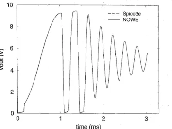
2.3. Algorithm 0 0 1 2 3 time (ms) Fig. 7NOWE and Spice3e.
Simulation results of nonlinearly loaded oscillator obtained by
By constructing and solving the derivative circuits successively, one can compute the time derivatives of the exact solution of branch currents and voltages. Note that, the linearized equivalent of the original circuit for the solution at t = O+ and the derivative circuits obtained by the construction described above differ only in the values of the independent sources. Therefore, the solution of the nth derivative circuit requires a forward and back substitution over the single LU decomposition performed at the beginning of the entire analysis. Unlike AWE analysis, in NOWE, all previous order derivatives are required for the computation of the values of the independent sources. The whole algorithm may be summarized
5
.r
: 3 EE
0$
.- as follows. G 2 \ \ \ \ \ ~ NOWE \ \ _ _ _ Trapezoidal App. \ \ \ \ \ \Find the dc solution 50 of the circuit at t = 0- while the
capacitors are open circuit and the inductors are short circuit. Note that this is the solution of zeroth time derivative circuit. Find all of the time derivatives of the voltages and currents in the circuit up to a desired order by the following steps.
2.1. Construct the first time derivative circuit and solve. The solution of this circuit yields the first time derivatives of the voltages and currents at t = O+.
2 . . .
2.n. Construct the nth derivative circuit and solve. The solutions of the all previous ( n - 1) derivative circuits are needed in the construction.
Find ( n - 1) st and nth order polynomial rational functions of time derivatives of which match to the derivatives computed in Step 2 for the storage elements and outputs under consideration. For voltages and currents of nonlinear elements, find nth order approximating polynomial rational functions.
Find a sufficiently small (but as large as possible) time step such that the following conditions hold. For storage elements, the normalized difference between the two successive approx- imation orders is less than a prescribed value. For nonlinear elements, the computed variables of the device satisfy the constitutive relations within a certain normalized error. Replace the energy storage elements by the appropriate inde- pendent sources whose values are equal to the last computed state variables (i.e., the capacitor voltages and the inductor currents) from Step 4. Go to Step 1. Use the solution of the circuit at the last time point as the seed of the new Newton-Raphson iteration.
Continue until the required time interval is covered.
G I
rn \ \1 ' I
-8 -6 -4 -2 0
log(max.
abs.
error)
Fig. 8. A typical relationship between the number of time steps required and the accuracy.
III.
EXAMPLESNOWE has been implemented in a computer program written in C++ and run on a SUN Sparcstation 10/40. Sparse Tableau Analysis formulation is selected for the sake of simplicity. Note that there is a significant penalty because of this selection.
The first example is a nonlinearly loaded oscillator with two bipolar transistors and three capacitors, and an inductor and four resistors. The simulation result of NOWE and the result obtained from Spice3e closely match, as depicted in Fig. 7 .
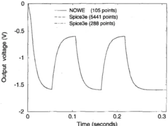
The second example is an ECL four-bit adder with 102 transistors, 34 diodes, and 364 resistors, and is simulated by using NOWE. The results are compared with the results obtained from Spice3e simulation which is run for various error criteria. The Sparse Tableau Analysis formulation results in a matrix size of 2036 x 2036 for this example. The relative error criterion is set to 10F4 for NOWE. Under this criterion, the maximum of the actual error appears to be less than lop5. The error is controlled by comparing the simulation results of two consecutive order approximations for the state variables. The error is also checked by evaluating the controlled variables of the
IEEE TRANSACTIONS ON COMPUTER-AIDED DESIGN OF INTEGRATED CIRCUITS AND SYSTEMS, VOL. 15, NO. 3, MARCH 1996
nonlinear devices. For example, for a device defined by i = f ( v ) ,
the error Jiapprox,mate - f ( ~ ~ is evaluated and controlled. ~ ~ ~ ~ ~ , ~ ~ ~ ~ ) ) There exist two means of increasing the accuracy: i) increasing the
order of approximation at each NOWE step and ii) decreasing the time interval between two consecutive NOWE steps. Our experimental implementation of NOWE keeps the order fixed and decreases the time step until the error is less than a predetermined limit. By this rule of error control, the total execution time is weakly dependent on the selected order. Moreover, increasing accuracy requirement causes a minimal increase in the required number of time steps and hence in the total execution time. However, unlike the Trapezoidal Approximation, the error limit should be kept below a certain value in order to obtain a convergent simulation result. To be on the safe side, this value should be chosen less than
The NOWE method may introduce serious problems for highly stiff circuits. Typical problems for simulation of stiff circuits by NOWE may involve an overflow in the high-order derivatives or too-small time steps. However, these problems may be overcome by destzffeening the circuit and/or by using a tight error control mechanism. Destiffening is achieved by inserting series resistors with parasitic capacitors and parallel resistors with parasitic inductors with time constants determined by the user supplied time step. The cost of this procedure is an increase in the size of the circuit and degradation in accuracy. However, it enables a fast solution of the circuit. Destiffening can be justified by its effect on the frequency- domain behavior of a linear circuit. One can easily show that this operation is equivalent to warping of the s-plane such that the poles and zeros with large magnitudes are shifted closer to the origin while those with small magnitudes remain almost untouched. Accordingly, a stiff circuit is observed as a nonstiff one in simulation. Moreover, one can easily show that integration using Forward Euler approximation after applying this kind of destiffening is equivalent to the integration by Trapezoidal Approximation.
The typical relationship between the number of time steps required and the accuracy is shown in Fig. 8 for a fourteenth order NOWE. Here the abscissa is the maximum absolute difference between the computed solution and the exact solution for a chosen output variable. In the same figure, the behavior of accuracy versus number of time steps for the Trapezoidal Approximation algorithm is depicted. In the Trapezoidal Approximation, to get two orders of magnitude in im- provement in accuracy, the number of time steps should be increased roughly by an order of magnitude. For the same improvement, NOWE requires a modest (10% N 15%) increase in the number of time
steps. Moreover, in NOWE, the Newton-Raphson analysis requires more iterations at each time point. This is due to the fact that the solution obtained for the new time point is used as a seed for the next Newton-Raphson analysis, and this seed having a smaller error requires a lesser number of Newton-Raphson iteration steps.
The simulation result of NOWE is shown in Fig. 3 along with the results obtained from a 228-point Spice3e run and a 5441-point Spice3e run. A zoomed view of this comparison is given in Fig. 10. The whole NOWE simulation involves 376 LU decompositions of the 2036 x 2036 sparse matrix and 3289 forward and back substitu- tions. These numbers include fourteenth order NOWE approximations at 105 time points. Each of NOWE approximations require 28 forward and back substitutions plus one LU. The rest of the LU and FBS count is accounted for Newton-Raphson iterations at each time point. Since NOWE yields an analytical function to be evaluated at each iteration point, the value of the output under consideration can be evaluated at any arbitrary time point.
Note from the Fig. 10 that the 105-point NOWE result matches closely the 5441-point Spice3e simulation, while it differs signif- icantly from the 229-point Spice3e run. Compared to 16 302 LU
0 -0.5
2
> -1 a 0 m 0 c-
c 3 fl c -1.56
~ 373 __ NOWE (105points) - _ - Spice3e (5441 points) Spice3e (288 points) -2 0 0.1 0.2 0.3 Time (seconds)Fig. 9. Simulations carry-out signal of a 4 b adder by NOWE and by Spice3e with various tolerances.
-0.596 -0.598
1
__ NOWE (105 points) Spice3e (5500 points) Spice3e (288 points)I,
-0.602 0.104 0.105 0.106 0.107 Time (seconds)Fig. 10. Comparison of NOWE and Spice3e2 results in a detailed view.
decompositions of 5441-point Spice3e simulation, and 1289 LU decompositions of 229-point Spice3e simulation, NOWE requires only 376 LU decompositions, demonstrating the efficiency of the proposed method. In this comparison, we have omitted the compu- tation time required for waveform approximation operations, e.g., coefficient recursions, Hankel matrix inversions, and nonlinear error control function evaluations, mainly due to the following reasons. The operations mentioned here are scalar operations. That is, the runtime corresponding to Hankel matrix inversions and the coefficient recursions grow linearly with the circuit size and quadratically in the order of the NOWE approximation. Second, these operations take less than 10% for each of the total runtime, even excluding the input parsing and output formatting for this example. The extra nonlinear function evaluations for error control takes less than 0.5% of the total runtime and this complexity is independent of the order of approximation. LU decomposition and FBS operations will dominate the CPU time as the circuit size grows, since their complexity depend on the circuit size super-linearly.
IV.
CONCLUSIONThe comparison of the number of LU decompositions of NOWE and the Spice3e simulations with various accuracy criteria show that
314 IEEE TRANSACTIONS ON COMPUTER-AIDED DESIGN OF INTEGRATED CIRCUITS AYD SYSTEMS, VOL. 15, NO. 3, MARCH 1996
NOWE technique reduces the number of LU decompositions without sacrificing the accuracy.
The experimental version of the simulator that we have written to implement the NOWE technique already has a comparable speed with Spice, although the present implementation uses Sparse Tableau Analysis for the purpose of simplicity. Use of Modified Nodal Analysis formulation would reduce the matrix size by approximately an order of magnitude. Therefore, a speed-up of at least an order of magnitude is expected.
Evaluation of the output values at any desired points not coinciding with the simulation time points can be achieved with a minimal additional cost-just the evaluation of a polynomial rational function. Our experiments by NOWE have shown that satisfactory results are obtained for approximation orders in the range 5 to 14. In this range, the simulation times vary at most by a factor of two.
The method presented in this paper has a great potential to replace the Trapezoidal Approximation used in conventional circuit simulators by the virtue of reduced number of LU decompositions at the expense of an increase in the number of Fl3S’s. This is an attractive property especially for very large circuits.
REFERENCES
[l] L. 0. Chua and P.-M. Lin, Computer-Aided Analysis of Electronic Cir- cuits: Algorithms and Computational Techniques. Englewood Cliffs, NJ: Prentice-Hall, 1975.
[2] L. T. Pillage and R. A. Rohrer, “Asymptotic waveform evaluation for timing analysis,” IEEE Trans. Computer-Aided Design, vol. 9, pp.
352-366, Apr. 1990.
131 B. R. Chawla, H. K. Gummel, and P. Kozah, “MOTIS-an MOS timing simulator,” IEEE Trans. Circuits. Syst., vol. CAS-22, pp. 901-909, Dec. 1975.
[4] C. F. Chen and P. Subramaniam, “The second generation MOTIS timing simulator-An efficient and accurate approach for general MOS circuits,” in Proc. Int. Symp. Circuits Syst., Montreal, P.Q., Canada, May 1984, 538-542.
[5] L. Vidigal, S. Nassif, and S. Director, “CINNAMON: Coupled INte- gration and Nodal Analysis of MOs Networks,” in Proc. 23rd Design Automation Con$, July 1986, 179-185.
[6] R. Bauer, J. Fang, A. Ng, and R. Brayton, “XPSim: a MOS VLSI simulator,” in Proc. Int. Con5 Computer-Aided Design, Santa Clara, CA, Nov. 1988, pp. 66-69.
[7] L. W. Nagel, “SPICE2: A computer-program to simulate semiconductor circuits,” University of California, Berkeley, Tech. Rep., Memo ERL- M520, May 1975.
[SI L. M. Silveira, J. K. White, H. Neot, and L. Vidigal, “On exponential fitting for circuit simulation,” IEEE Trans. Computer-Aided Design, vol. 11, pp. 566574, May 1992.
[9] C. T. Dikmen, M. M. Alaybeyi, S. Topcu, A. Atalar, E. Sezer, M. A. Tan, and R. A. Rohrer, “Piecewise linear aymptotic waveform evaluation for transient simulation of electronic circuits,” in Proc. Int. Symp. Circuits Syst., Singapore, June 1991, pp. 854-857.
[lo] M. H. Press, B. P. Flannery, S. A. Teukolsky, and W. T. Vetterling, Numerical Recipes in C. Cambridge, MA: Cambridge University, 1988.
[ 111 L. 0. Chua, C. A. Desoer, and E. S. Kuh, Linear and Nonlinear Circuits. New York McGraw-Hill, 1987.
[12] J. J. Bussgang, L. Ehrman, and J. W. Graham, “Analysis of nonlinear systems with multiple inputs,” IEEE Proc., vol. 62, pp. 1088-1119, Aug. 1974.