Determination of shelter locations and evacuation routes for a possible earthquake in the city of Istanbul

(1)

DETERMINATION OF SHELTER LOCATIONS AND EVACUATION ROUTES

FOR A POSSIBLE EARTHQUAKE IN THE CITY OF ISTANBUL

A THESIS

SUBMITTED TO THE DEPARTMENT OF INDUSTRIAL ENGINEERING

AND THE GRADUATE SCHOOL OF ENGINEERING AND SCIENCE OF BILKENT UNIVERSITY

IN PARTIAL FULFILLMENT OF THE REQUIREMENTS FOR THE DEGREE OF

MASTER OF SCIENCE

By

Ceyda Kırıkçı

(2)

I certify that I have read this thesis and that in my opinion it is full adequate, in scope and in quality, as a dissertation for the degree of Master of Science.

___________________________________ Prof. Dr. Barbaros Tansel (Advisor)

___________________________________ Assoc. Prof. Dr. Bahar Y. Kara

______________________________________ Asst. Prof. Dr. İbrahim Akgün

Approved for the Graduate School of Engineering and Science :

____________________________________ Prof. Dr. Levent Onural

(3)

ABSTRACT

DETERMINATION OF SHELTER LOCATIONS AND EVACUATION ROUTES FOR A POSSIBLE EARTHQUAKE IN THE CITY OF ISTANBUL

Ceyda Kırıkçı

M.S. in Industrial Engineering Supervisor: Prof. Dr. Barbaros Tansel

June, 2012

In this study, the location of disaster response and relief facilities in Istanbul is investigated in view of a possible earthquake. Our objective is to determine and analyze the assignments of demand nodes to shelter nodes. We propose two mathematical models for this purpose. Model 1 is a path based model, in which the possible paths are determined by preprocessing the network data to assign demands to shelters while obeying path capacities. Model 2 is an arc based model that uses the network data directly and creates the paths as a byproduct of the solution. Both of the models ensure that each demand node is served by at least a shelter node in accordance with road and shelter capacities. We examine the effect of the shelter capacity, the number of shelters, and the road capacities on the results in different cases. In these cases, we find out that the shelter capacity, number of shelters, and road capacities influence the shelters to be opened, the assignment of the demand nodes to these shelters and the used arcs/paths in this assignment.

Keywords: Evacuation, shelter location, humanitarian logistics, arc capacitated

(4)

ÖZET

OLASI BİR ISTANBUL DEPREMİNDE BARINMA YERLERİNİN YER SEÇİMİ VE TAHLİYE ROTALARININ BELİRLENMESİ

Ceyda Kırıkçı

Endüstri Mühendisliği Yüksek Lisans Tez Yöneticisi: Prof. Dr. Barbaros Tansel

Haziran 2012

Bu çalışmada , Istanbul’da afet müdahale ve yardım tesisleri yer seçimi, olası bir deprem açısından incelenmiştir. Bu çalışma kapsamındaki problem, barınma yerleri ve olası bir deprem sonrasında kullanılmak üzere tahliye yolları belirleme problemidir. Burada amaç insanları kısıtlı bir zamanda bulundukları coğrafi konumdan barınak noktalarına İstanbul’un metropol yol ağını kullanarak tahliye etmek ve izin verilen maksimum güzergah uzunlukları, barınak ve yol kapasiteleri gibi olası kısıtlara uyarak onların yolda geçecek sürelerini en aza indirmektir. Bunun için iki matematiksel model öneriyoruz. Model 1, uzunluk kısıtlı olası güzergahları girdi olarak alan bir tahliye modelidir. Model 2 ise ağ yapısını doğrudan kullanan serim akış bazlı bir modeldir ve güzergahları çözüm çıktısının bir parçası olarak sunar. Her iki model de, yol ve barınak kapasitelerine uyacak şekilde her talep noktasının en azından bir barınak noktasından hizmet aldığını garanti eder. Bu modeller, ayrıt ve barınak kapasitelerinin olduğu ve olmadığı ve tesis sayılarının değişik değerler aldığı farklı durumlar için çözülmüştür. Çözümlerde, tahliye sırasında fazla yığılma olan ayrıtlar ve tesisler belirlenmiş ve darboğaz yaratan ayrıt veya tesislerin deprem sonrası devre dışı kalması durumunda tahliye ve tesis yer seçimlerinin nasıl etkileneceği incelenmiştir.

Anahtar Kelimeler: Tahliye, barınma yerlerinin yer seçimi, insani yardım lojistiği,

(5)

ACKNOWLEDGEMENT

First of all, I would like to express my genuine appreciation to my supervisor Prof. Dr. Barbaros Tansel for his guidance and contributions. He has supervised me with everlasting patience and encouragement throughout this thesis. I consider myself lucky to have a chance to work with him. I owe thanks to Assoc. Prof. Dr. Bahar Y. Kara and Asst. Prof. Dr. İbrahim Akgün for their valuable revisions and constructive suggestions. In addition, I would like to thank Dr. Emrah Tufan for his valuable contribution to this study.

I am thankful to Önder Okyay for his support and encouragements inspired my continued excitement and dedication to this study.

I am grateful to my mother Hediye Kırıkçı, to my father Mehmet Zeki Kırıkçı and to my brother Mustafa Caner Kırıkçı, for their unconditional love and support throughout my life. I always felt their loving presence and trust.

I wish to express my sincere gratitude to Oğuzcan Samsun for his morale support, endless patience and encouragement during this study.

I would like to thank TÜBİTAK (The Scientific and Technological Research Council of Turkey) for supporting my graduate study through a scholarship.

Finally, I owe thanks to all my professors, friends and colleagues for their valuable company and contributions to my life. I have always been proud of being a member of Bilkent University-IE Department both as a student and an assistant.

(6)

LIST OF FIGURES

Figure 1 The Earthquake Models (Master Plan (2003)) ... 11

Figure 2 Initial demand nodes ... 12

Figure 3 Initial shelter nodes ... 13

Figure 4 The main roads ... 14

Figure 5 The Snapping Process ... 15

Figure 6 The Splitting Process ... 16

Figure 7 Preprocessed Network ... 17

Figure 8 The free flow for two unit arc length and free flow velocity of one unit length/unit time ... 20

Figure 9 The free flow for three unit arc length and free flow velocity of one unit length/unit time ... 21

Figure 10 An example for the enumeration of the paths in the path enumeration program .. 25

Figure 11 The assignment of demand points to shelter points in Model1_ii (r= 30 km) in Case-1 ... 34

Figure 12 The assignment of demand points to shelter points Model2_ii in Case-1 ... 35

Figure 13 The over-capacitated arcs for Model1_i (r=30 km) and Model2_i ... 40

Figure 14 The assignment for demand nodes, 1, 8, 28 and 30 in Case-1 ... 44

Figure 15 The assignment for demand nodes, 1, 8, 28 and 30 in Case-3 ... 44

Figure 16 The assignments for Model1_i with r=30 km in Case-1 ... 47

Figure 17 The assignments for Model1_i with r=30 km in Case-4 ... 47

Figure 18 Model1_i (r=30 km) in Case-1 ... 52

Figure 22 The over-capacitated shelters in Case-1 ... 57

Figure 23 The percentage of population that is assigned to a shelter versus the evacuation time t for Model1 ... 68

Figure 24 The percentage of population that is assigned to a shelter versus the evacuation time t Model2 ... 68

(9)

LIST OF TABLES

Table 1 The arc capacities for different unit times (t) ... 23

Table 2 The total number of paths and maximum number of paths between a demand and a shelter node as an input for Model1 ... 26

Table 3 The Cases that are analyzed ... 31

Table 4 Computational results of Models ... 33

Table 5 The assignment of the demand nodes to shelter nodes ... 35

Table 6 Shelter Utilization ... 38

Table 7 Arc Capacity Usage for Model1_i (r=30 km) and Model2_i ... 39

Table 8 Computational results of Model1 ... 41

Table 9 Computational Results of Model2 ... 42

Table 10 Computational results for Models ... 43

Table 11 Computational results for Model1 ... 45

Table 15 Computational results for Model1 (r=30 km) and Model2 ... 51

Table 18 Computational results for Model1 (r=30 km) and Model2 ... 56

Table 19 Computational results of scenario analysis for Model1 and Model2 (p=49) ... 58

Table 20 The Maximum Distance Data for the blockages of some shelters for the Models (t=24h and p=49) ... 59

Table 21 The Maximum Distance Data for Models for Case-5 (t=24h) ... 60

Table 22 Computational results of scenario analysis for Model1 and Model2 (p=49) ... 61

Table 23 The Maximum Distance Data for the blockages of some arcs for the Models (t=24h and p=49) ... 62

Table 24 Computational results of scenario analyses for Model1 and Model2 ... 63

Table 25 Computational results of scenario analysis for Model1(r=30 km) and Model2 (r=30 km) ... 64

Table 26 Computational results for Model1_iii (r=30 km) and Model2_iii. ... 67

Table 27 The summary of the results obtained from Model1_i and Model2_i for all cases .. 71

Table 28 The summary of the results obtained from Model1_ii and Model2_ii for all cases 72 Table 29 CPU times (in seconds) for the Models ... 73

(10)

Chapter 1

Introduction

There is an increase in the number of people who suffer from a disaster in recent years. This led the entire world to focus on pre-disaster and post-disaster planning. Disaster issue is also an important issue in Turkey. In particular, the expected earthquake in Istanbul requires more attention since Istanbul has 12.5% of the total population of Turkey and 50 % of the industrial potential of Turkey (Erdik and Durukal 2007). Hence, AKOM (Afet Koordinasyon Merkezi- Disaster Coordination Center), IMM (Istanbul Metropolitan Municipality) and Governorship of Istanbul have performed many projects and applications about pre-disaster and post-disaster activities. The Master Plan (2003) which is conducted by four universities (Bogazici University, ODTU, ITU and YTU) and JICA Report (2002) which is prepared by Japanese experts are the most comprehensive work done for an expected Istanbul Earthquake so far. They have investigated the Istanbul Earthquake in all aspects, such as the possible scenarios, the analysis of damages according to these scenarios, economical and social effects of the earthquake, etc.

Being prepared is essential for properly responding to devastating effects of an earthquake. Strengthening activities, emergency response management activities and training for public are some examples of preparation activities.

After an earthquake, quick and effective response to the needs of people is a critical issue. In that case, shelter locations become important. Note that, shelters can be described as emergency response facilities and relief centers that serve for health

(11)

locations in Istanbul and assignment of people to these shelters in case of an earthquake.

We propose two different models to determine the location of shelters and assignment of people to these shelters. Model 1 has a path based structure. We assume that people will use the paths which are predetermined in a distance limit of r to reach the shelter points. Model 2 is an arc based model and the model forms the paths to be used for assignment of demand points. In both models, we consider the shelter capacity, the number of shelters, and the road capacities as given. It is assumed in these models that everybody who needs accommodation is assigned to a shelter. The number of people at a given node may be partly assigned to different nodes, i.e. demand splitting is allowed.

In Chapter 2, we provide a literature review on disaster management in a wide-range. First, we introduce the studies about disaster management and humanitarians logistics, then we present the studies about location of emergency response facilities and relief centers.

In the models, we use the real road network and the real population data for İstanbul. To construct the network that is used in the proposed models, we made some assumptions and we preprocessed the real data. In Chapter 3, we introduce this process, the data that is used to handle the problem, and the structure of the problem, in detail. We provide detailed information on scenario determination for the earthquake, determination of demand nodes, shelter nodes, roads that will be utilized, and description of the capacities of demand nodes, shelters and roads.

In Chapter 4, we give the mathematical models that capture essential aspects of the problem.

In Chapter 5, we evaluate the effects of shelter capacity, number of shelters, and the road capacities on the optimal solutions obtained from the models. In this chapter, we introduce eight cases that differ according to the assumptions on shelter capacity, number of shelters, and the road capacities. Case-1 is the uncapacitated case, in

(12)

which shelters and roads are uncapacitated and the number of shelters is set to its upper limit 49. In Case-2, we obtain results for different numbers of shelters less than 49, assuming that shelters and roads are uncapacitated. Case-3 is the shelter capacitated case in which number of shelters is set to 49 and roads are uncapacitated. Case-4 is the road capacitated case, the number of shelters is set to 49 and the shelters are uncapacitated. In Case-5, Case-6, and Case-7, two of the parameters, shelter capacity, number of shelters, and the road capacities, are restricted and the remaining parameter is uncapacitated or taken as its upper bound in case of number of shelters. Finally, in Case-8 which is the more realistic case, shelters and roads are capacitated and the number of shelters is set to values smaller than 49.

In Chapter 6, we present a general conclusion about the study according to the computational results provided in Chapter 5. In Case-1 (Uncapacitated case), the demand nodes are assigned to the closest shelter nodes, due to the fact that the shelters are uncapacitated and p is set to its upper limit. The paths that are used for these assignments are the shortest paths, since the roads are also uncapacitated. However, in the other cases, the capacity of shelters and roads, and the restriction on number of shelters is considered. As a result, we generally obtain different results, in comparison to Case-1.

In Chapter 7, we provide the future work that will be done for this study as an extension. In the appendix, we give the data used in the models and the details of the computational results.

(13)

Chapter 2

Literature Review

In this part, we investigate the literature on two main issues. First, we handle the operations management literature in disaster and humanitarians logistics, to provide a general viewpoint on the subject. Then, we introduce the research in the literature about location of disaster response facilities and relief centers.

2.1. Disaster Related Operations Management and Humanitarians Logistics

The literature on disaster related operation management is generally related to social sciences. The sociological and psychological effects of a disaster on survivors, organizational design and communication problems etc. are investigated in this literature. From the viewpoint of operational research, the literature about disaster related operation management is restricted. However, especially in recent years (2000-2010) there is some progress in this area. Altay and Green (2006) provided a survey on the use of operational research models in disaster management. In this survey, the issues in disaster management and existing OR/MS literature in disaster management are investigated. According to the survey, 109 articles are published that are related to the issue. 77 of them are published in OR/MS related journals. 60 % of these papers are published after 2000, which supports the progress in this area in recent years. Actually, most of the research that will be reviewed in our study is after the year 2006 which indicates that disaster management has become an important issue owing to the augmentation of the natural and man-made disasters in the world. As a result, this area has turned into a more productive research area.

(14)

Kovacs and Spens (2007) provided a study on humanitarians logistics in disaster relief operations. They have created a framework determining a network between actors, phases and logistical processes of disaster relief. The unique characteristics of humanitarians logistics similar to business logistics are investigated. Preparedness, immediate response to disaster, reconstruction issues and supply network of humanitarian aid are included in the research.

Tomasini and Wassenhove (2009) conducted a case study on humanitarian logistics. The paper investigated the evaluation of supply chain management in disaster relief and the role of new players like private sector. They have addressed the preparedness, response and collaboration of a disaster in the view point of humanitarian supply chains. In disaster preparedness, reconstruction of the supply chain network, management of the resources and prepositioning of relief items are investigated to lessen the effects of a disaster. In disaster response, coordination of actors that must work together after a disaster is included. With the case study, they call attention to the importance of collaboration of the public and private sector in humanitarian logistics in a disaster.

Ergun and Karakus (2010) provided an introductory article which points out main characteristics of disaster supply chains and the issues that will be faced while managing them. Debris management operations are investigated in the perspective of operational research.

Ozdamar, Ekinci, and Küçükyazıcı (2004) conducted a research on emergency logistics and planning in natural disasters. The paper focused on the emergency logistics problem of distributing multiple commodities from a number of supply centers to the distribution centers that are close to affected areas. The aim of the study is to determine pick up and delivery schedules for vehicles and the quantities of loads delivered on these routes. To this end, a multi-period multi-commodity network flow model is developed. In light of this problem, the aim is to minimize the

(15)

sum of unsatisfied demand of all commodities in the planning horizon. An iterative lagrangian relaxation algorithm and a greedy heuristic are built up to solve the problem.

Another research related with emergency logistics is provided by Yi and Ozdamar (2007). In that study, a dynamic logistics coordination model is proposed for evacuation and support in disaster response activities. The problem that is addressed is to coordinate the transportation of commodities from supply centers to distribution centers that are close to affected areas and the transportation of injured people from affected areas to the temporary and permanent emergency response facilities. The model for the problem is a mixed integer multi-commodity network flow problem. The objective is to minimize the delay in the arrival of commodities at aid centers and the delay of supply of medical operations for the injured people. The study also includes a case study for Istanbul.

2.2. Emergency Response and Location of Disaster Response Facilities and Relief Centers

There are many local studies about emergency response and location of disaster response facilities and relief centers, such as Dekle et al. (2005) focused on the location of disaster recovery centers in Florida. The aim is to minimize the total number of disaster recovery centers needed, considering that each country resident is within a distance/radius r of the nearest disaster response unit. To deal with this problem a two-stage approach is proposed based on the covering location problem. Jia, Ordonez, and Dessouky (2007) provided a modeling framework for facility location of medical services for large-scale emergencies. First, the general facility location problems are surveyed to investigate the models used to focus common emergency situations, such as house fires, etc. Then, the characteristics of large-scale emergencies are determined and they are modeled in the perspective of general facility location model as a covering model, a p-median model and a p-center model according to different characteristics of large-scale emergencies. The models are

(16)

scenario based. The impact of the emergency on a demand point is stated in the model.

Balcik and Beamon (2008) conducted a study on facility location in humanitarian relief. The study focused on the location of distribution centers to satisfy the needs of the people affected by quick-onset disaster. The number and location of distribution centers and the amount of relief inventory that will be stocked considering the maximization of the satisfaction of people needs are the main issues of the problem. A maximal covering location problem approach is proposed to solve the problem. The relief items that will be stocked and distributed are assumed to be in multiple types and they are weighted according to their importance and their target response times. Network reliability is not considered in the study. The research is scenario-based which means that the uncertainties about the disaster locations and demand quantities are reflected to the model with scenarios. In the model, a single demand unit and multiple capacitated supplier units are assumed. The objective is to maximize the total expected demand covered by established distribution centers. Cheng and Tzeng (2007) conducted a study on multi-objective optimal planning for designing relief delivery systems. The relief distribution model has three objectives: minimizing the total cost, minimizing the total travel time, and maximizing the minimal satisfaction during the planning period. Temporary storage units and two-stage transportation model are suggested. A fuzzy multi-objective linear programming formulation is developed to solve the problem.

Görmez, Köksalan, and Salman (2010) considered a case study on locating response facilities in Istanbul. Istanbul metropolitan municipality proposed 40 potential locations for response facilities after an earthquake. The criteria for determining these potential areas is accessibility by at least two alternative roads, closeness to major highways and the availability of land. A two-tier distribution system utilizes the public facilities as temporary facilities that will serve as local distribution and coordination center after a disaster. It uses the new facilities as permanent facilities

(17)

temporary facilities from which the demand point requirements are satisfied. In this flow the failure of the links are not taken into consideration. There are two assumptions in the construction of model: the facilities located have sufficient capacities and the new facilities will survive after an earthquake. This model is also scenario based. In the first stage of the model temporary facility locations and the allocation of demand points to temporary facilities are determined by minimizing the demand-weighted distance. In the second stage, the locations of permanent facilities to serve demands are determined by minimizing the average distance travelled to serve a demand point and the number of new facilities to establish.

There is not so much a study on disaster management with network reliability. If the link failures are considered, the disaster management problem can become more complicated. The study of Rawls and Turnquist (2009) considers issues related to network reliability. They have focused on pre-positioning of emergency supplies for disaster response. The problem is to determine facility locations for emergency response, the stock levels for emergency items and distribution of these items to multiple demand locations after an event. In this study, the uncertainty is considered and reflected to the problem definition in all aspects. Uncertainty about demand, the situation of prepositioned stocks and the condition of transportation network is considered in the model. A two-stage stochastic mixed integer program is developed to formulate the model. The model is scenario based, and the probability of scenarios is introduced to the model. The aim is minimizing the expected cost over all scenarios. The cost is formed by these components: the cost resulting from the selection of the pre-positioning locations and facility sizes, the commodity acquisition and stocking decisions, the shipments of supplies to demand points, unsatisfied demand penalties, and holding costs for unused material.

Hassin, Ravi, and Salman (2010) conducted a study on facility location on a network with unreliable links. The research focused on locating emergency response units on a network considering random link failure after a potential earthquake. Link failure among arcs is assumed to be dependent. The objective is to satisfy as much demand

(18)

as possible within a time /distance limit. A demand point can be covered, if a facility exits within a specified distance to the demand point. An exact Dynamic programming algorithm and an exact greedy algorithm are developed for the problem with no distance limit.

(19)

Chapter 3

Problem Definition

In this part, we provide the data that is used to comprehend the problem and discuss the assumptions that are used to construct the models. First, we present detailed information on scenario determination for the earthquake. Then, we determine the demand nodes, shelter nodes, the roads that will be utilized and the construction of the network. We also describe the capacities of the demand nodes, the shelters and the roads.

3.1. Scenario Determination

After a likely Istanbul earthquake, there are a lot of uncertain issues, e.g., the damages of the earthquake on the road network and the buildings, the amount and location of people that will be affected by the earthquake etc. We introduce this uncertainty to the models by determining a scenario on the likely Istanbul earthquake.

In this study, we form the data that is used in constructing the models according to the scenario in Model A which is defined in Master Plan (2003) as the most probable scenario.

Master Plan (2003) defines four scenarios according to the magnitude of the earthquake and the location of the fault. In Figure 1, the location of the fault can be seen for all models. Model A which is suggested to be the most probable scenario

(20)

has a magnitude estimation of 7.5 on the Richter Scale. The magnitude of the scenario in Model B, C and D is estimated to be 7.4, 7.7 and 6.9 Richter Scale, respectively.

This assumption influences the location and the portion of the population that will need a shelter after a likely earthquake. We assume that Istanbul road network is not affected.

Figure 1 The Earthquake Models (Master Plan (2003))

3.2. Network Construction

In this part; we describe the demand nodes, shelter nodes, the roads and the details about construction of the network.

We realize the construction of the network in two main steps: i) Initial Network Construction:

(21)

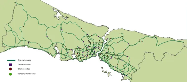
We select the districts of Istanbul as demand nodes. Note that, each demand node represents the number of people who may need accommodation in the aftermath of a likely Istanbul earthquake. There are 39 districts in Istanbul and each demand node is located at the administrative centers of the districts. However, “Adalar” district is left out of the demand set since we only deal with the Istanbul road network and there is no road connection between “Adalar” node and the other nodes. So, we have 38 demand nodes. We show the initial demand nodes in Figure 2.

Figure 2 Initial demand nodes

We tabulate the detailed information for demand nodes in Appendix 1.

Through interviews with IMM, 49 potential shelter location points are determined as shelter nodes. The shelters can be described as disaster response and relief facilities. They are permanent accommodation areas -6-8 months- and health units for people. They include storage units that will pre-store emergency response items including tents, medical equipment, dry food water, etc.

We illustrate these nodes with the help of electronic data (IMM 2006) that is introduced in ArcMap and with the help of GoogleMaps. Note that, open areas and

(22)

parks form these potential shelter nodes. The initial set for the shelter nodes is shown in Figure 3.

Figure 3 Initial shelter nodes

We show the information about shelter points in Appendix 2.

To comprehend the structure of the Istanbul road network, we investigate the current road data in GoogleMaps and construct the network in ArcMap. While developing the Istanbul road network, we consider the main roads (highways and large streets). The network consists of 318 edges and 209 road junction nodes. Note that the intersection of three or more roads constitutes a road junction point. The road network can be seen in Figure 4.

(23)

Figure 4 The main roads

Let V0 be the node set with V0=F0 U D0 U N where F0 is the set of nodes that represent the potential shelter nodes, D0 is the set of nodes that represent the demand nodes and N is the set of nodes that represent the transshipment nodes that are neither demands nor potential shelters.

Let E0 be the edge set. The edge set includes only the main roads of the Istanbul Road Network.

The initial network G0= (V0, E0) is an undirected network and includes 296 nodes (38 demand nodes, 49 shelter nodes and 209 transshipment nodes) and 318 edges.

During the development of the initial network, we ignore the rural roads, so most of the nodes in F0 U D0 are not located on E0. To construct a network in Arcmap with the main roads, we preprocessed the initial network.

(24)

ii) Preprocessed Network:

To construct the network in Arcmap, the demand and the shelter nodes are projected/snapped to the edge set, so that the resulting network possesses demands arising at nodes and snapped nodes of the final network. Note that “Snap” is a tool that projects the selected nodes to the nearest point of the closest line in ArcMap. To clarify the issue, we state an example for the snapping process.

(green = before snapping, red = after snapping)

Figure 5 The Snapping Process

In this simple example, four nodes occur near a line and one point is already on the line (Figure 5-A). The Snap tool is run with a snap tolerance high enough to allow all the nodes to be snapped to the line (Figure 5-B). Figure 5-C shows both sets of nodes.

Let ai be the distance between original location of ith node and its snapped point on

the network. While constructing the distance data, we also consider ai. The data about

ai is tabulated in Appendix 4.

After the snapping operation, the initial edge data is split by the snapped demand and shelter nodes into new edges. We realize this operation with the help of the tool “Split Line at a Point” in Arcmap. This tool splits the lines, based on intersection or proximity to nodes. Since all the nodes are snapped to the edge set, there is no need to define a distance value for proximity.

(25)

(green = before splitting, red = after splitting)

Figure 6 The Splitting Process

In this example, four nodes are located near a line and one point is already on the line in Figure 6-A. In this situation, the line is split by a point which is on the line and there are two edges. After the snapping operation, all the nodes are projected on the line and the line is divided into 5 edges (Figure 6-B).

In our network, at the end of these processes, demand nodes and shelter nodes are snapped to the edge set. Then, the edge set is split according to the snapped nodes. Note that preprocessed network includes 296 nodes and 407 edges.

Let G’=(V,A) be a directed network with vertex set V and arc set A where V=F U D U N s.t F is the set of nodes that represent preprocessed shelter nodes, D is the set of nodes that represent preprocessed demand nodes and N is the set of nodes that represent the transshipment nodes formed by the road junction nodes. A is constructed so that each undirected edge {i,j} in E is replaced by a pair of directed arcs (i,j) and (j,i) of the same length. Additionally, the same capacity is assigned to both directed arcs. As a result, we have 814 arcs in our network.

296 nodes in V are numbered in such a way that the first 38 are the demand nodes. The shelter nodes are numbered from 39 to 87 and the rest of the nodes are numbered 88 to 296. The details about numbering process can be seen in the Appendix. The preprocessed network is shown in the Figure 7.

(26)

Figure 7 Preprocessed Network

We show the arcs and the length of the arcs in Appendix 3.

3.3. Determination of Demand Amounts

We use the population values from TUIK (Turkiye Istatistik Kurumu) for 38 district nodes to determine the demand amounts. In master plan, there is a study on “Percentage of people that may need accommodation after Istanbul earthquake in Model A” which is shown in Appendix 5. In that study, only a part of Istanbul is investigated and we can obtain the information about the percentage of people that may need accommodation for some of the districts. The analyzed part of Istanbul is considered to be more likely to be affected by the earthquake. For this reason, we assume for the districts not included in the master plan study to be affected by 5% of their population. The list of demand nodes and their demand amounts are tabulated in Appendix 1.

3.4. Determination of Shelter Capacities

(27)

maximum number of people that can be served by this shelter. Note that the service capabilities of the shelters are identical.

The shelters include the health units for people and the storage units that will pre-store emergency response items (tents, medical equipment, dry food water etc.). These units and items may be placed at shelters before or after the earthquake. Shelters can be constructed and receive the items to be stored before the earthquake, which provides an advantage for preparedness. However, the constructed units and stored items can be damaged by the earthquake, and also the potential shelter areas can be utilized for other issues. Alternatively, they can be constructed and receive the supplies after the earthquake. In this case, the constructed units and stored items are not damaged. However, it may take time to construct such a shelter.

We do not investigate the issues related to the construction of these units and the storage of the items in this study. We assume that the shelters are constructed before the earthquake and will not be damaged by the earthquake. Accordingly, it is assumed that there will be no capacity loss after the earthquake.

To calculate the shelter capacities, we use the available areas of potential shelter locations as their capacities. The list of shelter nodes and their capacities are tabulated in Appendix 2. These capacities are calculated according to the approximate areas of the possible shelter locations and the assumption “4 people can accommodate in a 50 m2_{pre-fabric room”. For example, for shelter node “39”, the}

approximate area is 596000 m2 and the capacity of the shelter is calculated as:

The capacity of shelter node “39” = (596000 m2 / 50 m2 ) * 4 people = 47680 people Capacities of shelters change in the range of 47680–76000 people.

3.5. Determination of Arc Capacities

In this part, we describe the arc capacities.

An arc’s capacity is taken to be the maximum number of cars that can pass through the arc in free flow conditions in unit time.

(28)

The parameters that can influence the capacity of an arc are stated below: ¾ The length of the arc

¾ The structure of the arc (the number of lanes, width of the arc, and the physical structure etc.)

¾ The free flow velocity of the car ¾ The unit time t

We assume that the structure of the arc, the free flow velocity of the car and the unit time t are the same for all the arcs. So, the only factor that distinguishes the arcs in our network is the length of the arcs. We simulate the free flow of the cars on an arc to investigate the effect of the arc length on the arc capacity.

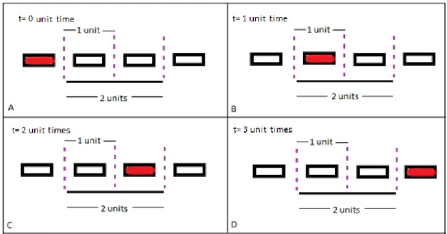
In this basic simulation, we take the free flow velocity as one unit length/unit time. The length of the arcs and the length of the spacing that a car needs (including its own length) in free-flow are determined in terms of “unit arc length”. The t value determined in terms of “unit time” and taken as three unit times. To steer to the left and to change the lane are not allowed and all roads are in free flow when the flow starts between demand nodes to shelter nodes.

(29)

Figure 8 The free flow for two unit arc length and free flow velocity of one unit

length/unit time

The discrete flow is shown for unit time intervals. The rectangles represent the cars and the line which has a two unit length represents an arc in the network. One of the cars is colored with red and with the help of this car, the flow of the cars on the arc can be seen clearly. The spacing of the car, including its own length is one unit length. Only one direction of the road is handled in this example, for the fact that the other side will also show the same behavior. In each Figure 8-A, 8-B- 8-C and 8-D, 1 unit advance of the red colored car can be seen. In Figure 8-A, the car is just about to enter the arc, in Figure 8-B and in Figure 8-C it flows through the arc and finally it leaves the arc in Figure 8-D. In 3 unit time, 3 cars can pass through the arc. According to this, the capacity of the arc is:

3 cars/3unit time = 1 car/ unit time

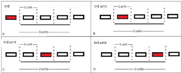
For further investigation, we change the arc length from two unit length to three unit length in Figure 9.

(30)

Figure 9 The free flow for three unit arc length and free flow velocity of one unit

length/unit time

In Figure 9, only the arc length is different from Figure 8 and the arc length is 3 unit length. In Figure A, the car is just about to enter the arc, in Figure B, in Figure 9-C and in Figure 9-D it flows through the arc. In 3 unit time, 3 cars can pass through the arc. According to the simulation, the capacity of the arc is:

3 cars/3unit time = 1 car/ unit time

According to the examples the capacity of the road remains the same while the length of the arc changes. As a result, it can be said that, the capacity of an arc is independent of the length of the arc.

An arcs capacity can also be calculated without a simulation with the help the following formula in the light of our assumptions:

Arc capacity (in cars)=(unit time t) / ((The spacing of a car)/ (The free-flow velocity of a car))

In this study, we do not consider how (the sequence of the flow of the cars, etc.) the demand amount flows through the arcs to the shelter nodes in the unit time. We only

(31)

determine the amount of cars that can pass through an arc in free flow conditions in unit time.

We state the assumptions for determination of the capacity of the arcs in our network below:

• The free flow velocity is 60 km/h.

• A car needs a spacing of 30 meters (including its own length) in free-flow. • All roads are bidirectional, single lane, have the same width and both sides

have equal capacity.

• To steer to the left and to change the lane are not allowed.

• All roads are in free flow when the flow starts between demand nodes to shelter nodes.

• 5 people can travel in a vehicle.

• The capacity of an arc is not affected by the blockage of the road due to the earthquake.

According to these assumptions and basic simulation, the structure of the arc, the free flow velocity of the cars are the same and the length of the arcs does not affect the capacity. We can conclude that all the arcs in our network have the same capacity. We use t which is the elapsed time for evacuation of people, as the unit time for capacity calculation. With the help of this, we determine the arc capacity that is the number of the cars that can pass through the arc in free flow conditions in the elapsed time for evacuation of people. In the models, we take the t value as 6h, 8h, 12h, 24h, 36h, 48h, 60h and 72h. Rt is introduced to the models as the capacity of the arc for

the elapsed time t in terms of people. The arc capacities for different t values are tabulated in Table 1.

(32)

Table 1 The arc capacities for different unit times (t)

t (h) Arc Capacity (cars) Rt

(people) 6 12000 60000 8 16000 80000 12 24000 120000 24 48000 240000 36 72000 360000 48 96000 480000 60 120000 600000 72 144000 720000

In the models to evacuate people. For example for t= 8h, we calculate the capacity of an arc:

Arc Capacity = (8 h)/ (30 m /60.000 m /h) = 16000 cars Rt = (Arc Capacity)*5 people = 80000 people

where the free flow velocity is 60 km/h, the spacing of a car is 30 meters (including its own length) in free-flow and we assume that 5 people travel in a car.

In our study we assume single lanes. If we have considered the multiple lanes for the arcs, the calculation of the capacity of the arc can be:

(33)

Chapter 4

Mathematical Models

In this part, we introduce the mathematical models that are developed for Shelter Location Problem. The mathematical models can be classified into two groups, these are:

• Path Based Models • Arc Based Models

4.1. Model 1 (Path Based Model)

Model 1 is the model that handles the problem with a path based structure in which the flow from demand nodes to shelters can be realized by the paths that are predetermined. In determination of these paths, alternative paths are investigated between a demand node and a shelter node, within a distance limit r.

The paths under consideration are simple paths, so it is not difficult to enumerate them when the path length is restricted to an upper bound r that corresponds to the maximum length of a path from a demand node to a shelter node. The code for the enumeration of length restricted simple paths for the İstanbul Network is developed by Tufan (2011).

The inputs to the code are the sets of demand nodes, shelter nodes, arcs with their lengths, the depth of the enumeration tree and the r value that restricts the lengths of the paths to be enumerated. The program searches for all length restricted paths between a demand node and shelter nodes that are acceptable in the specified depth of the enumeration tree.

(34)

In Figure 10, we show an example for the enumeration of paths between demand node 1 and the set of shelter nodes. Only one branch of the tree is given in the figure. The depth of the tree is 5 and the r value is set to 10 km.

Figure 10 An example for the enumeration of the paths in the path enumeration

program

In the example, we could see that the program searches for a shelter node starting from the demand node 1, for the depth value 5 according to the criteria that the path lengths are not longer than 10 km. For the branch that is shown in the example, the program finds the following paths:

¾ 1-39-159-41, with the path length 2600 m.

¾ 1-39-159-158-18-40, with the path length 6739 m. ¾ 1-39-159-158-155-43, with the path length 7398 m.

(35)

When the program enumerates the shelter node 41, it stops since there is no node to enumerate after node 41 that satisfies the upper bound of r=10 km on the path length.

This enumeration process is realized for all the demand nodes. As a consequence, we obtain all paths between the set of demand nodes and the set of shelter nodes that are admissible within the upper bound of r and within the specified depth of the tree.

The depth of the tree for the paths that are used is important for the models. The computational program attempts to enumerate all paths between a demand node and a shelter node with increasing tree depth. However, the CPU times and the memory bounds increase with increasing tree depth. For a depth ≥ 15, it was not possible to get an output from the program. Accordingly, we select the depth of tree as 14 for all path calculations. The set of paths so obtained gives a reasonably good approximation of the set of all paths that are admissible within the length restriction of r.

In Table 2, we tabulate the total number of paths for r values and the maximum number of paths between a demand and a shelter node that are found by the computational program of Tufan (2011).

Table 2 The total number of paths and maximum number of paths between a demand

and a shelter node as an input for Model1

r (km)

Maximum Number of Paths between a Demand Node and a

Shelter Node Total Number of Paths 16 98 3004 20 195 7718 25 251 13891 30 251 17365

(36)

In our network, we use the main roads in the arc set construction which made our network sparse. Accordingly, we utilize 3004 (for r=16 km), 7718 (for r=20 km), 13891 (for r=25 km) and 17365 (for r=30 km) paths as input for Model1.

Model 1 ensures that each demand point is covered by at least one shelter within distance r. We take into account shelter and arc capacities. Demand splitting is allowed. According to two different objectives; Model 1_i and Model 1_ii are formed.

Parameters:

eikzab 1 if the arc (a,b) is in the zth path that connects the nodes i and k

0 o.w.

dikz Length of zth path between nodes i and k.

wk Demand (affected population) of demand point k. Ci Capacity of shelter i (in terms of number of people). r Upper bound on path lengths.

Rt The capacity of an arc in unit time t (in terms of number of people)

(t=6h, 8h, 12h, 24h, 36h, 48h, 60h and 72 h).

p Upper bound on number of shelters.

Decision Variables:

xikz amount of demand k satisfied by shelter i with path z. yi 1 if shelter i is opened

(37)

Model 1-i : s.t. (1) (2) (3) (4) (5) (6)

In Model 1_i, the total distance travelled by people is minimized. (1) ensures that each demand point is covered by at least one shelter within a path of length at most r. (2) ensures that the people are served by a shelter in the capacity limit of the shelter if that shelter is opened. (3) puts an upper bound on the number of shelters that will be opened. (4) satisfies the edge capacity. Constraint (5) states that xikz are

nonnegative variables and (6) states variables are binary variables.

Model 1_ii is the same as Model 1_i except that the objective function is changed to the minimization of the number of shelters to be used. Additionally, the third constraint of Model 1_i is dropped.

Model 1-ii : Min s.t. (1), (2), (4), (5), (6).

4.2. Model 2 (Arc Based Model)

Model 2 is the arc capacitated version of the multicommodity flow formulation of the p-median problem proposed by Tansel and Akgün (2010).

(38)

To construct the model, a new node, node 0, is added, to G=(V,A) and arcs (i,0) are added to the arc set A for each i F. Let G* = (V*, A*) be the resulting directed network.

Let k D and define a supply of wk units at each demand node k D for commodity

k. Note that each demand node k is treated as a supply point (origin) for commodity type k. Define a demand of wk units for commodity k at node 0 where node 0 is a

sink for each commodity. As a result, wk units of flow will be delivered from node k

D to node 0 via directed paths that visit at least one of the shelter nodes. Denote by lij the length of arc (i,j). We assign the length 0 to arcs (i,0) for all i.

In the formulation below, we take into account the shelter and arc capacities. Note that demand splitting is allowed.

We remove the distance bound r from the problem and solve the arc capacitated problem to minimize the total distance travelled subject to an upper bound constraint on the number of shelters that can be used.

In this model, we use the parameters and variable yi that are described in Model2.

The variables xijk are defined as follows:

xijk : the flow of commodity k in arc (i,j) where (i,j) A* and k D.

Model 2-i : s.t. (7) (8) (9)

(39)

(10) (11) (12) (13) (14) (15)

In Model 2_i, the total distance travelled by people is minimized.

(7) is the flow balance constraint at node 0 for commodity k. (8) is the flow balance constraint at every other node i for commodity k. (9) ensures node k is served by a shelter i only if i is an open shelter. (10) puts an upper bound on number of shelters that will be opened. (11) ensures the total flow (population) served by shelter i is no more than its capacity. (12) is the arc capacity constraint. (13), (14) are nonnegativity constraints and (15) is the 0/1 constraint.

In Model 2_ii, the number of open shelters to evacuate all population will be minimized. Model 2_ii is the same as Model 2_i except that objective function is changed and constraint (10) in Model 2_i is dropped.

Model2-ii

(40)

Chapter 5

Computational Results

In Model1 and Model2, there are three important parameters that affect the results. These are number of open shelters (p), shelter capacities, and arc capacities. In this section, the computational results of different values of these parameters are investigated. Note that upper limit for p is 49.

We examine the cases that are stated in Table 3.

Table 3 The Cases that are analyzed

CASE p Shelter Capacities Arc Capacities 1 49 Infinite Infinite 2 < 49 Infinite Infinite 3 49 Finite Infinite 4 49 Infinite Finite 5 49 Finite Finite 6 < 49 Finite Infinite 7 < 49 Infinite Finite 8 < 49 Finite Finite

In order to analyze the cases above, we investigate some important metrics which are obtained from the output of the models that are implemented on GAMS. The computer that is used for this purpose has a processor Intel Pentium CPU U5400 @ 1.2 GHz and its memory is 4 GB. The operating system of the computer is Windows

(41)

The metrics that are used in the analyses are:

Average and maximum distance travelled by people to reach the shelters they are assigned.

Number of shelters that must be opened. Shelter capacity usage

Arc capacity usage

The assignment of people that are at demand points to shelter points and the assigned population amounts

The arcs/paths that are used for the assignment of the demand points to shelter points.

5.1. Analysis of Results for Case-1

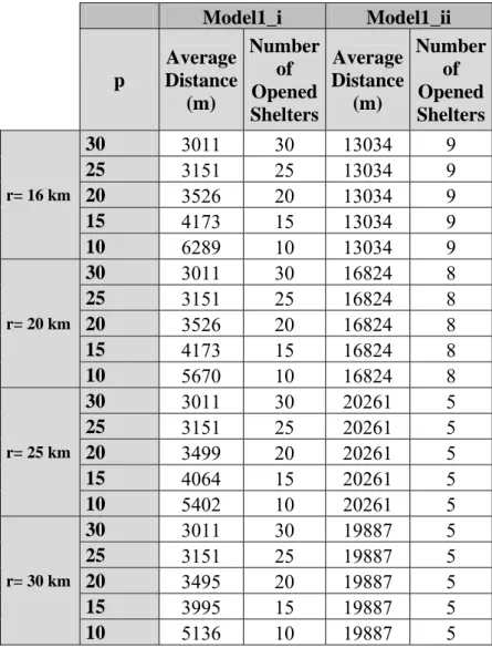
In Case-1, shelters and arcs are uncapacitated and p value is set to its upper limit 49. The length of the paths between the east end and the western end of Istanbul is approximately 100 km. During the evacuation, it is expected that most people will use paths to reach a shelter that are close to their home locations. With a diameter of 100 kilometers, it is reasonable to restrict path lengths to values of r ranging between 15 to 30 kilometers. The values of r that are used in model 1 are 16, 20, 25, and 30 kilometers.

The results corresponding to Model1_i and Model1_ii for r values 16 km, 20 km, 25 km and 30 km and the results corresponding to Model2_i and Model2_ii are tabulated in Table-2 in order to compare these models in terms of the average distance travelled per person and the number of opened shelters.

In Case-1, we expect that the demand points will be assigned to their closest shelter points since shelters are uncapacitated. Also, the paths that are used for these assignments will be shortest paths due to the fact that arcs are uncapacitated.

(42)

In the other cases, take into account capacities and have a chance to compare these results with Case-1 which is the uncapacitated case.

Table 4 Computational results of Models

Model1_i Model1_ii Average Distance (m) Maximum Distance (m) Number of Shelters Opened Average Distance (m) Maximum Distance (m) Number of Shelters Opened r= 16km 3011 15427 30 13034 15863 9 r=20 km 3011 15427 30 16824 19854 8 r=25 km 3011 15427 30 20261 24910 5 r=30 km 3011 15427 30 19887 29352 5 Model2_i Model2_ii Average Distance (m) Maximum Distance (m) Number of Shelters Opened Average Distance (m) Maximum Distance (m) Number of Shelters Opened 3011 15427 30 56995 78456 1

In Table 4, the results of Model1_i are the same for all r values. There is no capacity restriction on the model. So, the shortest paths are selected for the assignment of the demand points. The shortest paths and the assignments are the same for all r values since the paths in r =16 km are contained by other r values greater than r=16 km. Model2_i is an arc based model and considers all possible paths without an r limit. So, the same results are obtained.

For Model1_ii and Model2_ii, the objective is to minimize the number of shelters. In Model1_ii, there is an inverse relationship between average distance travelled per person and the number of opened shelters. As r increases, the number of shelters decreases or stays the same; in return, the average distance travelled increases. However, the situation for r=25 km and r=30 km are different. The number of shelters obtained are the same but the average travelled distance for r= 30 km is smaller. The primary reason for that is that the set of paths within a limit of r=25 km is included as a subset of the set of paths with a limit of r=30 km. This gives more

(43)

of shelters to open that satisfies all the constraints and minimizes the number of shelters. In the current case, the model finds shorter paths for more populated demand points for r=30 km and the average distance travelled becomes smaller with the same number of shelters.

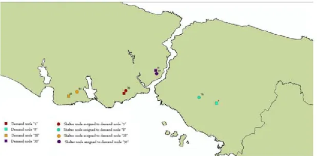
In Model1_ii, the number of the shelters can be minimized up to five shelters within defined r limits. In Model2_ii, one shelter suffices to serve all demand points in the uncapacitated case since Model2_ii assigns the demand points to shelter points without considering any r limit on the paths. In our graph each node is accessible from all other nodes, so the model opens a shelter and assigns all the demand nodes to this shelter. The model searches the shelter nodes starting from 39 to 87. The shelter node with the number 39 is opened as it gives the minimum total distance to serve the entire population. The demand node 6 which represents “Şile” district is also assigned to shelter node 39 with the path length 78456 m which is the maximum length for the model. We show the assignments for Model1_ii and Model2_ii in Figure 11 and Figure 12.

Figure 11 The assignment of demand points to shelter points in Model1_ii (r= 30

(44)

Figure 12 The assignment of demand points to shelter points Model2_ii in Case-1

The assignment of the demand nodes to shelter nodes and assigned demand amounts is tabulated in Table 5.

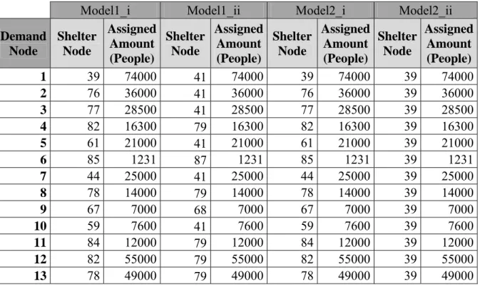
Table 5 The assignment of the demand nodes to shelter nodes

Model1_i Model1_ii Model2_i Model2_ii

Demand Node Shelter Node Assigned Amount (People) Shelter Node Assigned Amount (People) Shelter Node Assigned Amount (People) Shelter Node Assigned Amount (People) 1 39 74000 41 74000 39 74000 39 74000 2 76 36000 41 36000 76 36000 39 36000 3 77 28500 41 28500 77 28500 39 28500 4 82 16300 79 16300 82 16300 39 16300 5 61 21000 41 21000 61 21000 39 21000 6 85 1231 87 1231 85 1231 39 1231 7 44 25000 41 25000 44 25000 39 25000 8 78 14000 79 14000 78 14000 39 14000 9 67 7000 68 7000 67 7000 39 7000 10 59 7600 41 7600 59 7600 39 7600 11 84 12000 79 12000 84 12000 39 12000 12 82 55000 79 55000 82 55000 39 55000 78 49000 79 49000 78 49000 39 49000

(45)

Model1_i Model1_ii Model2_i Model2_ii Demand Node Shelter Node Assigned Amount (People) Shelter Node Assigned Amount (People) Shelter Node Assigned Amount (People) Shelter Node Assigned Amount (People) 14 51 115000 41 115000 51 115000 39 115000 15 79 54000 79 54000 79 54000 39 54000 16 63 32000 41 32000 63 32000 39 32000 17 77 31500 79 31500 77 31500 39 31500 18 40 68000 41 68000 40 68000 39 68000 19 45 55000 41 55000 45 55000 39 55000 20 41 108000 41 108000 41 108000 39 108000 21 70 30000 41 30000 70 30000 39 30000 22 54 22000 41 22000 54 22000 39 22000 23 44 23000 41 23000 44 23000 39 23000 24 74 9000 79 9000 74 9000 39 9000 25 68 4000 53 4000 68 4000 39 4000 26 55 9000 53 9000 55 9000 39 9000 27 61 36000 41 36000 61 36000 39 36000 28 54 10000 41 10000 54 10000 39 10000 29 71 8000 41 8000 71 8000 39 8000 30 61 17000 41 17000 61 17000 39 17000 31 42 50000 41 50000 42 50000 39 50000 32 46 12000 41 12000 46 12000 39 12000 33 47 70000 41 70000 47 70000 39 70000 34 48 130000 41 130000 48 130000 39 130000 35 43 88000 41 88000 43 88000 39 88000 36 53 69000 41 69000 53 69000 39 69000 37 78 18000 79 18000 78 18000 39 18000 38 69 9000 53 9000 69 9000 39 9000

In Table 5, the assignments of demand points to shelter points regarding Model1_i, Model1_ii for the r value 30 km and Model2_i and Model2_ii are tabulated. For Model1, r=30 km is selected since the case r=30 km gives the closest results to Model2. The assignments, assigned amounts of the demand points and the paths are the same for Model1_i and Model2_i. The reason for this situation is that the shortest paths are selected to reach the shelter points since the arcs are uncapacitated. Due to the fact that all the shortest paths for the nodes exist in both of the models, Model1_i

(46)

and Model2_i give the same results. The arcs used in the assignment of Model1 and Model2 are tabulated in Appendix 6, Appendix 7, and Appendix 8. If we compare the assignments in Model1_i and Model1_ii, we see that a demand node that is assigned to a shelter in Model1_i may be assigned to a different shelter in Model1_ii. For example; the demand node 1 is assigned to the shelter node 39 in Model1_i, however it is assigned to the shelter node 41 in Model1_ii due to their objective functions. The same situation is also valid for Model2.

(47)

Table 6 Shelter Utilization Shelter No Actual Shelter Capacity Total Number of People Assigned Utilization Percentage Total Number of People Assigned Utilization Percentage Total Number of People Assigned Utilization Percentage Total Number of People Assigned Utilization Percentage 39 47680 74000 155% 0 0% 74000 155% 1424131 2987% 40 48000 68000 142% 0 0% 68000 142% 0 0% 41 56000 108000 193% 1135100 2027% 108000 193% 0 0% 42 60000 50000 83% 0 0% 50000 83% 0 0% 43 48000 88000 183% 0 0% 88000 183% 0 0% 44 64000 48000 75% 0 0% 48000 75% 0 0% 45 28000 55000 196% 0 0% 55000 196% 0 0% 46 64000 12000 19% 0 0% 12000 19% 0 0% 47 40000 70000 175% 0 0% 70000 175% 0 0% 48 40000 130000 325% 0 0% 130000 325% 0 0% 49 36000 0 0% 0 0% 0 0% 0 0% 50 64000 0 0% 0 0% 0 0% 0 0% 51 68000 115000 169% 0 0% 115000 169% 0 0% 52 64000 0 0% 0 0% 0 0% 0 0% 53 80000 69000 86% 22000 28% 69000 86% 0 0% 54 28000 32000 114% 0 0% 32000 114% 0 0% 55 64000 9000 14% 0 0% 9000 14% 0 0% 56 72000 0 0% 0 0% 0 0% 0 0% 57 64000 0 0% 0 0% 0 0% 0 0% 58 72000 0 0% 0 0% 0 0% 0 0% 59 64000 7600 12% 0 0% 7600 12% 0 0% 60 64000 0 0% 0 0% 0 0% 0 0% 61 28000 74000 264% 0 0% 74000 264% 0 0% 62 37600 0 0% 0 0% 0 0% 0 0% 63 68000 32000 47% 0 0% 32000 47% 0 0% 64 56000 0 0% 0 0% 0 0% 0 0% 65 80000 0 0% 0 0% 0 0% 0 0% 66 80000 0 0% 0 0% 0 0% 0 0% 67 52000 7000 13% 0 0% 7000 13% 0 0% 68 56000 4000 7% 7000 13% 4000 7% 0 0% 69 64000 9000 14% 0 0% 9000 14% 0 0% 70 72000 30000 42% 0 0% 30000 42% 0 0% 71 80000 8000 10% 0 0% 8000 10% 0 0% 72 64000 0 0% 0 0% 0 0% 0 0% 73 72000 0 0% 0 0% 0 0% 0 0% 74 72000 9000 13% 0 0% 9000 13% 0 0% 75 72000 0 0% 0 0% 0 0% 0 0% 76 40000 36000 90% 0 0% 36000 90% 0 0% 77 56000 60000 107% 0 0% 60000 107% 0 0% 78 80000 81000 101% 0 0% 81000 101% 0 0% 79 80000 54000 68% 258800 324% 54000 68% 0 0% 80 96000 0 0% 0 0% 0 0% 0 0% 81 88000 0 0% 0 0% 0 0% 0 0% 82 80000 71300 89% 0 0% 71300 89% 0 0% 83 72000 0 0% 0 0% 0 0% 0 0% 84 72000 12000 17% 0 0% 12000 17% 0 0% 85 80000 1231 2% 0 0% 1231 2% 0 0% 86 72000 0 0% 0 0% 0 0% 0 0% 87 76000 0 0% 1231 2% 0 0% 0 0% Model2_ii Model2_i Model1_ii Model1_i

As it can be seen from Table 6, some of the shelters are over-capacitated. Especially, for Model1_ii and Model2_ii the number of shelters number is minimized and the true capacities of opened shelters are highly exceeded as we allowed infinite capacities in Case-1. With the help of these results, we conclude that if the capacity

(48)

of over-capacitated shelters is obeyed, we expect to obtain different results in terms of the average distance travelled and the number of shelters.

If we summarize Table 6, the over-capacitated shelters are: ¾ For Model1_i; 39,40,41,43,45,47,48,51,54,61,77 and 78, ¾ For Model1_ii; 41,79

¾ For Model2_i; 39,40,41,43,45,47,48,51,54,61,77 and 78, ¾ For Model2_ii; 39

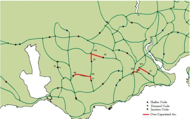
In Table 7, we show the over-capacitated arcs and usage percentages according to different t values in Model1_i (r=30 km) and Model2_i, the results are the same for both models.

Table 7 Arc Capacity Usage for Model1_i (r=30 km) and Model2_i

Node i Node j Flow Amount (People) Usage Percentage for t=8h Usage Percentage for t=12h Usage Percentage for t=24h 34 145 130000 163% 108% 54% 145 48 130000 163% 108% 54% 14 51 115000 144% 96% 48% 20 167 108000 135% 90% 45% 164 41 108000 135% 90% 45% 166 164 108000 135% 90% 45% 167 166 108000 135% 90% 45% 35 146 88000 110% 73% 37% 146 43 88000 110% 73% 37%

In Table 7, we can see the over-capacitated arcs for Model1_i and Model2_i for different arc capacity values (t=8h, 12h and 24h). If the capacities of these arcs are considered in the models, we expect to obtain different results in terms of average distance travelled by people.

(49)

Figure 13 The over-capacitated arcs for Model1_i (r=30 km) and Model2_i

In Figure 13, we show some of the over-capacitated arcs for Model1_i (r=30 km) and Model2_i for t= 8h.

The flow amounts on the arcs as an output of Model1_ii and Model2_ii are tabulated in Appendix 6. Most of the arcs that are used are over-capacitated according to the t values 8h, 12h, 24h, 36h and 48h. The aim is to minimize the number of shelters and all demand amounts flow through the same arcs to reach the small number of shelters.

In the following cases, the capacities of shelters and arcs and the number of shelters p are taken into account. As expected, the results are not better than Case-1 in terms of average distance and number of shelters. In the following sections, we investigate the effect of the capacities on the results.

(50)

5.2. Analysis of Results for Case-2

In Case-2, computational results are obtained for different values of p. Shelters and arcs are uncapacitated. In this case, we expect to analyze the effect of p on the results. The number of opened shelters will decrease or stay the same with decreasing p values. The possible changes on the shortest paths that are used for assignments and on the opened shelters are investigated.

To determine the effect of p on the results, p=30, 25, 20, 15 and 10 are introduced the models. In Table 8, the results are tabulated for Model1_i, Model1_ii and in Table 9 the results are shown for Model2_i and Model2_ii.

Table 8 Computational results of Model1

Model1_i Model1_ii p Average Distance (m) Number of Opened Shelters Average Distance (m) Number of Opened Shelters r= 16 km 30 3011 30 13034 9 25 3151 25 13034 9 20 3526 20 13034 9 15 4173 15 13034 9 10 6289 10 13034 9 r= 20 km 30 3011 30 16824 8 25 3151 25 16824 8 20 3526 20 16824 8 15 4173 15 16824 8 10 5670 10 16824 8 r= 25 km 30 3011 30 20261 5 25 3151 25 20261 5 20 3499 20 20261 5 15 4064 15 20261 5 10 5402 10 20261 5 r= 30 km 30 3011 30 19887 5 25 3151 25 19887 5 20 3495 20 19887 5 15 3995 15 19887 5

(51)

Table 9 Computational Results of Model2 Model2_i Model2_ii p Average Distance (m) Number of Opened Shelters Average Distance (m) Number of Opened Shelters 30 3011 30 56995 1 25 3121 25 56995 1 20 3465 20 56995 1 15 3934 15 56995 1 10 4822 10 56995 1

As it can be seen from Table 9, when p value decreases, the number of opened shelters decreases. As a result, average distance increases in Model1_i. For each p value, the number of opened shelters equals p. The reason for this situation is that the objective of Model1_i is to minimize the average distance travelled by people. So, to assign the demand points to the closest shelters, the number of shelters is set to its upper limit.

If we compare the results of Model1_i and Model2_i in this case with Model1_i and Model2_i in Case 1, the average distance values are greater in this case owing to the fact that some of the demand points cannot be assigned to the closest shelters since they cannot be opened due to the restriction on p.

For Model2_ii, the average distance travelled and the number of shelters does not change due to p, because the optimum number of facilities is smaller than p value. If we select a p value smaller than the optimum number of facilities for each model, we obtain infeasible solutions.

Model2 yields better results than Model1for r=30 km, 25 km, 20 km and 16 km, in terms of the optimal objective function values. To obtain the same results with Model2, in Model1 r should be set to the longest path in Model2 for this case or a greater value. However, this value can change with parameter changes.