Results in Physics 24 (2021) 104124
Available online 5 April 2021
2211-3797/© 2021 The Authors. Published by Elsevier B.V. This is an open access article under the CC BY license (http://creativecommons.org/licenses/by/4.0/).
Fractional stochastic sır model
Badr Saad T. Alkahtani
a, Ilknur Koca
b,*aDepartment of Mathematics, Riyadh, 11989, College of Science, King Saud University, P.O. Box 1142, Saudi Arabia
bDepartment of Accounting and Financial Management, Seydikemer High School of Applied Sciences, Mugla Sıtkı Kocman University, Mugla, Turkey
A R T I C L E I N F O Keywords:
Caputo Atangana-Baleanu
Caputo-Fabrizio differential operators Global derivative
Existence and uniqueness Numerical approximations
A B S T R A C T
Stochastic and fractional differentiation have been developed independently to depicting processes following randomness and power, a declining memory and passage from one process to another respectively. Very recently, fractional stochastic differential equations were suggested with the aim to capture processes following at the same time randomness and memory nonlocality. In this paper to further explore the applicability of this type of differential equations, a SIR model was considered and analyzed analytically and numerically. Some numerical simulations are presented for different values of fractional orders and densities of randomness.
Introduction
In the last decades few mathematical tools and concepts have been utilized to predict real world problems, for example classical differential and integral operators, fractional differential and integrals operators and stochastic-differential equations. They have been used for many different purposes. For example classical differentiation and integration have been used for modelling classical mechanical problems were memory is not captured. Indeed with these two mathematical operators many real world have been modelled with some limitations. Stochastic differential equations, have been used to modelling complex real world problems following randomness. Fractional calculus was introduced as extension of classical derivative, they have been introduced to replicate complex problems following power law processes, a declining memory and a passage from one process to another steady and non-steady states. In particular, these concepts have been applied to model epidemiolog-ical problems. The spread of many infectious diseases have been modelled and simulated, in some case the mathematical models have been compared with experimental data [1–4,9–11]. In some situation, the mathematical models were in good agreement with experimental data, clear indication that mathematical models were able to replicate accurately. However in many situation, modellers observed a clear disagreement between the observed data and the mathematical equa-tions. In these cases two questions could be asked the first question is to know if the collected data were done accurately, and the second one will be is the mathematical model suitable to model this situation? Now if the answer of the first question is yes, meaning the experimental data were
collected accurately, then clearly the mathematical models should be questioned. Indeed the spread of infectious diseases among humans is a serious worry and have reduced human population through death in the last past years. We can list few including Spanish flu that left many millions of death, HIV, syphilis, Ebola, malaria, dengue fever, Lassa fever, and covid-19 and its variants [19–25]. One main way to control their spread is perhaps to suggest a mathematical model that will be able to accurately replicate the spread such that its future can be predicted. Is the predictions are accurate, one could take decisions on how to control the spread. Very recently, Atangana and Seda suggested the use of fractional stochastic differential and integral equations [18]. This approach is very effective for modelling spread of infectious disease that follows processes with non-locality and randomness. In this paper, we analyse a mathematical model display the spread of some infectious diseases with fractional stochastic approach.
Fractional differentiation
In this section, we remember some important definitions for frac-tional derivative with local and non-local kernels [5–8,13].
Definition 1. Caputo fractional derivative of order α>0 of a function f : (0, ∞)→R, according to Caputo, the fractional derivative of a
continuous and differentiable function f is given as:
CDα tf ( t ) = 1 Γ(1 − α) ∫t 0 (t − x)−αd dxf ( x ) dx, 0 <α⩽1.1 (1) * Corresponding author.
E-mail addresses: [email protected] (B.S.T. Alkahtani), [email protected] (I. Koca). Contents lists available at ScienceDirect
Results in Physics
journal homepage: www.elsevier.com/locate/rinp
https://doi.org/10.1016/j.rinp.2021.104124
Definition 2. The Riemann–Liouville fractional integral of order α>0
of a function f : (0, ∞)→R, according to Riemann–Liouville, the frac-tional integral that is considered as anti-fracfrac-tional derivative of a func-tion f is: Iα tf ( t ) = 1 Γ(α) ∫t 0 (t − x)α−1f ( x ) dx, x > a.2 (2)
Definition 3. Let f ∈ H1(a, b), b > a, 0 <α<1 then, the new Caputo derivative of fractional derivative is defined as:
CF a D α tf (t) = 1 1 − α ∫t a f′ ( x ) exp [ − α(t − x) 1 − α ] dx.3 (3)
and also if the function does not belongs to H1(a, b) then, the derivative can be reformulated as CF a Dαtf (t) = α 1 − α ∫t a ( f ( t ) − f ( x )) exp [ − α(t − x) 1 − α ] dx.4 (4)
Theorem 1:Let 0 <α<1 then the following time fractional
ordi-nary differential equation
CF 0 D α tf (t) = u ( t),5 (5)
has a unique solution with taking the inverse Laplace transform and using the convolution theorem below:
f ( t ) =2(1 − α) (2 − α)u ( t ) + 2α (2 − α) ∫t 0 u ( s ) ds, t⩾0.6 (6)
Definition 4. Let f ∈ H1(a, b), b > a,α∈ (0, 1) then, the definition of the new fractional derivative is given as:
ABC a D α tf (t) = B(α) 1 − α ∫t a f′ ( x ) Eα [ − α(t − x) α 1 − α ] dx, 7 (7) where ABC
a Dαt is fractional operator with Mittag–Leffler kernel in the Caputo sense with order αwith respect to t and
B ( α ) =1 − α+ α Γ(α),8 (8) is a normalization function.
Definition 5. Let f ∈ H1(a, b), b > a,α∈ (0, 1) and not differentiable then, the definition of the new fractional derivative is given as:
ABR a D α tf (t) = B(α) 1 − α d dt ∫t a f ( x ) Eα [ − α(t − x) α 1 − α ] dx.9 (9)
Definition 6. The fractional integral of order α∈ (0, 1) of a new fractional derivative is defined as:
AB a I α tf ( t ) =1 − α B(α)f ( t ) + α B(α)Γ(α) ∫t a f ( y ) (t − y)α−1dy.10 (10)
When αis zero, initial function is obtained and when αis 1, the or-dinary integral is obtained.
The following time fractional ordinary differential equation
ABC 0 D α tf (t) = u ( t),11 (11)
has a unique solution with taking the inverse Laplace transform and using the convolution theorem below:
f ( t ) =1 − α B(α)u ( t ) + α B(α)Γ(α) ∫t a u ( y ) (t − y)α−1dy.12 (12)
Definition 7. Let f(t) be continuous, g(t) be a non-constant increasing
positive function. And also taking K(t) as kernel with singular or non- singular versions. For 0 <α⩽1, a fractional global derivative of Caputo sense is defined by
C 0D α gf (t) = Dgf (t)*K ( t ) 13 (13)
Also with Riemann–Liouville version, we have
RL
0 D
α
gf (t) = Dg(f (t)*K(t) ), 14 (14)
where * means the convolution operator.
We have to note that definitions above given with global idea are obtained very early by Atangana. You can see detailed analysis for global derivative in his paper referenced with [5]. Let us see some versions of its below.
Global derivative with Caputo version is given by
C 0D α gf ( t ) = 1 Γ(1 − α) ∫t 0 Dgf ( x ) (t − x)−αdx, 0 <α⩽1.15 (15)
Global derivative with Riemann–Liouville version is given by
RL 0 D α gf ( t ) = 1 Γ(1 − α)Dg ∫t 0 f ( x ) (t − x)−αdx, 0 <α⩽1.16 (16)
Global derivative with Caputo-Fabrizio version is given by
CF 0 Dαgf (t) = 1 1 − α ∫t 0 Dgf ( x ) exp [ − α(t − x) 1 − α ] dx.17 (17)
And finally global derivative with Atangana-Baleanu versions are given by ABC 0 Dαtf (t) = B(α) 1 − α ∫t 0 Dgf ( x ) Eα [ − α(t − x) α 1 − α ] dx, 18 (18) ABR 0 D α gf (t) = B(α) 1 − αDg ∫t a f ( x ) Eα [ − α(t − x) α 1 − α ] dx.19 (19)
In numerical proofs integral versions of those derivatives below are used, so integral operators with global derivative with Riemann–Liou-ville version is given by
0Iα gf ( t ) = 1 Γ(α) ∫t 0 g′ ( x ) f ( x ) (t − x)α−1dx.20 (20)
Caputo-Fabrizio version is given by
CF 0 I α gf (t) = 1 − α M(α)g ′ ( x ) f ( x ) + α M(α) ∫t 0 g′ ( x ) f ( x ) dx.21 (21)
Atangana-Baleanu version is given by
AB 0 I α gf ( t ) =1 − α B(α)f ( t ) g′ ( t ) + α B(α)Γ(α) ∫t a g′ ( x ) f ( x ) (t − x)α−1dx.22 (22)
Model derivation of stochastic SIR epidemic model
Although deterministic differential equations have been used inten-sively to replicate the spread of some infectious diseases, nevertheless, a day by day collection of data showed that, their spread sometime follow non-locality and randomness. A clear indication that neither fractional differential equation nor stochastic differential equations cannot be used to replicate such spread. Indeed if the spread follows randomness then stochastic differential equations are suitable for modelling such
prob-lems. Some published papers involving the use of stochastic differential equations can be found in [1–4]. In general the differentiation with randomness is given as below:
dx = f1(t, x, y)dt + f2(t, x, y)dw, 23 (23)
here wi = [w1,…,wn], for i = 1, …, n is an independent Wiener process. In the SIR model, s(t) is susceptible, i (t) is infective and r(t) is removed individuals in the population and given below
.s(t) = Λ − μs(t) − βs(t)i (t), (24) .i ( t ) = βs(t)i (t) − (μ+γ + ∊)i (t), .r(t) = γi (t) − μr(t).
The above Eq. (24) is the transform into stochastic, by adding invironment of noise.
ds(t) = [Λ − μs(t) − βs(t)i (t)]dt − w1s(t)dB1(t),
di (t) = [βs(t)i (t) − (μ+γ + ∊)i (t)]dt + w2i (t)dB2(t),
dr(t) = [γi (t) − μr(t)]dt + w3r(t)dB3(t)
where (wi)i=1,2,3 are densities of randomness and Bi(t)i=1,2,3are inviron-ment of noise.
All parameters above are positive constants. Also Λis the birth rate, μis the death rate, βis the average number of contacts per infective per day, γis the recovery rate and ∊is the death rate of infectives caused by disease.
0.1. Equilibrium point and stability analysis SIR epidemic model
In this subsection we can analyze the dynamics of the stochastic models with the help of the stability analysis of the deterministic equations. In fact, the solution to the deterministic model corresponds to the mean of the stochastic model. ˙In this subsection, firstly we study on deterministic SIR model to obtain equilibrium points and also we analyze sufficient conditions under which the equilibrium points are locally stable. Let us consider model below:
ds(t) dt =Λ − μs ( t ) − βs ( t ) i ( t ) , (25) di (t) dt = βs(t)i (t) − (μ+γ + ∊)i (t), dr(t) dt = γi (t) − μr(t).
Here if n(t) show total population size in dynamic, we calculate n(t) with following calculation. dn(t) dt = ds(t) dt + di (t) dt + dr(t) dt .26 (26) So we have dn(t) dt =Λ − μs ( t ) − μi ( t ) − ∊ + ( t ) − μr ( t ) , (27) ⩽ Λ − μs(t) − μi (t) − μr(t), ⩽ Λ − μn(t).
Then we will write
dn(t) dt +μn ( t ) ⩽Λ.28 (28)
Let us calculate inequality above with considering equality as
dn(t) dt +μn ( t ) =Λ.29 (29)
It’s a linear differential equation above so we have to find Lagrange
multiplier first. The multiplier is calculated as
λ = e
∫ μdt=
eμt.30 (30)
If we do necessary calculations then we have
n ( t ) =Λ μ+ce −μt.31 (31)
If we consider n(0) = 0, we will have
n ( t ) =Λ μ(1 − e −μt)32 (32)
For ∀t⩾0, we have that
n ( t ) ⩽Λ μ.33 (33) γ = ⎧ ⎨ ⎩ (s(t), i (t), r(t)) ∈ R3 +:s ( t)⩾0, i(t)⩾0, r(t)⩾0, n ( t ) =s ( t ) + i ( t ) +r ( t ) ⩽Λ μ ⎫ ⎬ ⎭,
region is positive invaryant for the system. Also for t→∞ lim t→∞ supn ( t ) ⩽Λ μ.34 (34)
So all the solutions of system is uniformly bounded in γ.
1. Equilibrium points
In this section, we derive the equilibrium points for both disease-free and endemic The disease-free equilibrium is given as E0 =
( Λ μ,0,0
) , for
i =0. The endemic equilibrium is obtained by solving the following
system. Λ − μs*− βs*i*=0, (35) βs*i*− (μ+γ + ∊)i*= 0, γi*− μr*= 0. Then we have s*=(μ+γ + ∊) β , i *=βΛ − μ(μ+γ + ∊) (μ+γ + ∊) ,r *=γ(βΛ − μ(μ+γ + ∊)) − μ(μ+γ + ∊) .36 (36) So endemic equilibrium point
E* ( s*, i*,r* ) =((μ+γ + ∊) β , βΛ − μ(μ+γ + ∊) (μ+γ + ∊) , βΛ − μ(μ+γ + ∊) (μ+γ + ∊) ) .
1.0.1. Local and global stability of the endemic equilibrium
First we consider Sır model as below
ds(t) dt =f1 ( s, i , r ) , (37) di (t) dt = f2(s, i , r), dr(t) dt = f3(s, i , r). Here f1(s, i , r) = Λ − μs(t) − βs(t)i (t), (38) f2(s, i , r) = βs(t)i (t) − (μ+γ + ∊)i (t), f3(s, i , r) = γi (t) − μr(t).
equilibrium J ⎛ ⎝E* ⎞ ⎠ = ⎡ ⎣− μ− βi * − βs* 0 βi* βs*− (μ+γ + ∊) 0 0 γ − μ ⎤ ⎦39 (39)
We now construct a characteristic equation associated to SIR model
k = det[J(E*) − λI] = 0.40 (40)
From the above, we obtain the following characteristic polynomial
k(λ)=λ3+k1λ2+k2λ + k3,41 (41)
where
k1=3μ+γ + ∊ + βi*− βs*, (42)
k2= μ2− 2μβs*+μβi*+(μ+γ + ∊)(2μ+βi*),
k3= (μ+γ + ∊)(μ2+μβi*)− μ2βs*.
Theorem: At the endemic equilibrium point E*(s*, i*,r*)is locally
asymptotic stable if all the eigenvalues λ1,λ2 and λ3 satisfy the following
condition |argλi|〉
απ
2fori = 1, 2, 3.43 (43)
Proof: If all the coefficients in the characteristic equation are
posi-tive (λi>0 for i = 1, 2, 3) then the system is asymptotically stable. The
matrix H is Hurwitz matrix, that is, all the real parts of the eigen values are in the left half plane so the above condition can be satisfied by Routh-Hurwitz criteria [14–17].The Hurwitz matrix for the character-istic polynomial k(λ) is written as
H3= ⎡ ⎣k11 k3k2 00 0 k1 k3 ⎤ ⎦44 (44) Then we have H1=k1>0, H2=k1k2− k3>0.45 (45)
So the proof is completed.
1.0.2. Global stability of the endemic equilibrium point
We present the global stability of the system
.s(t) = Λ − μs(t) − βs(t)i (t), (46) .i ( t ) = βs(t)i (t) − (μ+γ + ∊)i (t), .r(t) = γi (t) − μr(t).
We define in the classical case
.L =1 l1.i = βs(t)i (t) − l1i (t) l1 , (47) =(βs(t) − l1)i (t) l1 ,l1= ( μ+γ + ∊ ) . Then we write .L(t) = ( βs(t) l1 − 1 ) i ( t ) , (48) = (R0− 1)i ( t ) ,R0=βs * l1 .
Therefore, for all three cases
.L(t) = 0ifR0=1, (49)
.L(t) < 0ifR0<1,
.L(t) > 0ifR0>1.
Theorem: If R0⩾1, the endemic point E*(s*, i*,r*) is globally asymptotically stable.
Proof:We prove this using the idea of a fractional Lyapunov function.
We start by defining the Lyapunov function associated the system as below: L ( s*, i*,r* ) = ( s − s*+s*logs * s ) + ( i − i*+ i*logi * i ) + ( r − r* +r*logr * r ) ,50 (50) .L(t) =(s − s * s ) .s + ( i − i* i ) .i +(r − r * r ) .r, (51) = (s − s * s ) (Λ − μs(t) − βs(t)i (t)) + ( i − i* i ) (βs(t)i (t) − (μ+γ + ∊)i (t)) +(r − r * r ) (γi (t) − μr(t)). Then we write .L(t) = Λ +μs*+βsis * s+βsi + ( μ+γ + ∊ ) i*+μr*+γi (52) − ( Λs * s+μs + βsi + ( μ+γ + ∊ ) i + βsi*+μr +γi r * r = Π1− Π2, where Π1=Λ +μs*+βsis * s+βsi + ( μ+γ + ∊ ) i*+μr*+γi , (53) Π2=Λ s* s+μs + βsi + ( μ+γ + ∊ ) i + βsi*+μr +γi r * r . Therefore if Π1− Π2>0then.L(t) > 0, (54) Π1− Π2= 0then.L(t) = 0, Π1− Π2< 0then.L(t) < 0.
2. Analysis of SIR stochastic model
In this section, we consider a general SIR stochastic model where the classical time derivative is convertal to global derivative. Noting a global derivative of a differentiable function f with respect to an increasing non-negativecontinuous function g is defined
Dgf ( t ) =limt→t1f (t) − f (t1) g(t) − g(t1).
Indeed if g is differentiable then
Dgf ( t ) =f ′ (t) g′ (t).
Let us consider following stochastic SIR model,
ds(t) = [Λ − μs(t) − βs(t)i (t)]dt − w1s(t)dB1(t), (55)
di (t) = [βs(t)i (t) − (μ+γ + ∊)i (t)]dt + w2i (t)dB2(t),
dr(t) = [γi (t) − μr(t)]dt + w3r(t)dB3(t)
persistence of the disease. s(t) and i (t) and r(t) are positive solutions for
t⩾0 of system above for any given initial value (s(0),i (0),r(0)) ∈ R3
+. Also s ( t ) + i ( t ) +r ( t ) ⩽Λ μ,56 (56) for t⩾0.
But now we consider system of stochastic differential equations with global derivative first
Dgs
(
t)=[Λ − μs(t)− βs(t)i(t)]− σs(t)i(t), (57) Dgi
(
t)= [βs(t)i (t) − (μ+γ + ∊)i (t)] +σs(t)i (t),
Dgr
(
t)= [γi (t) − μr(t)],
s(0) = s0, i (0) = i0 and r(t) = r0.
Since g is differentiable, then we can write
ds(t) = [Λ − μs(t) − βs(t)i (t)]g′(t)dt − w1s(t)g′(t)dB1(t), (58)
di (t) = [βs(t)i (t) − (μ+γ + ∊)i (t)]g′(t)dt + w2i (t)g′(t)dB2(t),
dr(t) = [γi (t) − μr(t)]g′(t)dt + w3r(t)g′(t)dB3(t)
Its worth noting that if the environmental noiser (wi)i=1,2,3=0 then
the model is simple shetor ministic.
Applying the integral on both sides, we have
s ( t ) =s ( 0 ) + ∫t 0 g′ ( τ ) (Λ − μs(τ) − βs(τ)i (τ))dτ (59) − ∫t 0 g′ ( τ ) (σs(τ)i (τ))dτ, i (t) = i(0)+ ∫t 0 g′ ( τ ) (βs(τ)i (τ) − (μ+γ + ∊)i (τ))dτ + ∫t 0 g′ ( τ ) (σs(τ)i (τ))dτ, r ( t ) =r ( 0 ) + ∫t 0 g′ ( τ ) (γi (τ) − μr(τ))dτ+w3 ∫t 0 g′ ( τ ) r ( τ ) dB3 ( τ ) .
Now with the idea of Brownian motion, we have
s ( t ) =s ( 0 ) + ∫t 0 g′ ( τ ) (Λ − μs(τ) − βs(τ)i (τ))dτ (60) − ∫t 0 g′ ( τ ) (σs(τ)i (τ))dB(τ), i (t) = i(0)+ ∫t 0 g′ ( τ ) (βs(τ)i (τ) − (μ+γ + ∊)i (τ))dτ + ∫t 0 g′ ( τ ) (σs(τ)i (τ))dB(τ), r ( t ) =r ( 0 ) + ∫t 0 g′ ( τ ) (γi (τ) − μr(τ))dτ+w3 ∫t 0 g′ ( τ ) r ( τ ) dB3 ( τ ) .
Thus, with classical global derivative we have the following nonlinear stochastic equation. Let us present now the condition under which the nonlinear case has unique solution which is taking advantage of Atangana’s paper referenced by [5,6].
Theorem: Assume that there are four positive constants α1 ,α1,α2,α2,α3 and β1,β1,β2,β2,β3 such that.
i) |f1(t, s) − f1(t, s1)|2⩽α1|s − s1|2, (61) |f2(t, s) − f2(t, s1)|2⩽α1|s − s1|2 and also |g1(t, i ) − g1(t, i1)|2⩽ α2|i − i1|2, |g2(t, i ) − g2(t, i1)|2⩽ α2|i − i1|2, |h1(t, r) − h1(t, r1)|2⩽α3|r − r1|2. ii) |f1(t, s)|2⩽ β 1 ( 1 + |s|2), |f2(t, s)|2⩽ β1 ( 1 + |s|2), |g1(t, i )|2⩽ β2 ( 1 + |i |2), |g2(t, i )|2⩽ β2 ( 1 + |i |2), also |h1(t, r)|2⩽β3 ( 1 + |r|2).
Proof of Lipschitz condition for equations of SIR model: In this
part we reconsider stochastic model as below
ds(t) = f1(t, s(t))dt + f2(t, s(t))dB(t), (62) di (t) = g1(t, i (t))dt + g2(t, i (t))dB(t), dr(t) = h1(t, r(t))dt + h2(t, r(t))dB(t). Here f1(t, s(t)) = Λ − μs(t) − βs(t)i (t), (63) f2(t, s(t)) = − σs(t)i (t), g1(t, i (t)) = βs(t)i (t) − (μ+γ + ∊)i (t), g2(t, i (t)) = σs(t)i (t), h1(t, r(t)) = γi (t) − μr(t).
Now we define the following norm ‖ϑ‖∞= sup
t∈[0,T]
|ϑ|2,
then we have ∀s, s1∈R2 and t ∈ [0,T]
|f1(t, s) − f1(t, s1)|2= |( − μ− βi (t))(s − s1) |2, (64) ⩽ {2μ2+2β2|i (t)|2}| s − s1|2, ⩽ { 2μ2+2β2t∈[0,T]sup|i (t)|2}| s − s1|2, ⩽ {2μ2+2β2‖i (t)‖2 ∞ } |s − s1|2,⩽α1|s − s1|2.
where α1= {2μ2+2β2‖i (t)‖2∞}. And
|f2(t, s) − f2(t, s1)|2= |( − σi (t))(s − s1) |2, ⩽ {σ2|i (t)|2}| s − s1|2, ⩽ { σ2t∈[0,T]sup|i (t)|2}| s − s1|2, ⩽ {σ2‖i (t)‖2 ∞ } |s − s1|2,⩽α1|s − s1|2, where α1 = { σ2‖i (t)‖2∞ }
.Also we show that ∀i , i1∈R2 and t ∈ [0, T] then |g1(t, i ) − g1(t, i1)|2= |(βs(t) − (μ+γ + ∊))(i − i1) |2, (65) ⩽ {2β2|s(t)|2+ 2(μ+γ + ∊)2}|i − i1|2, ⩽ { 2β2t∈[0,T]sup|s(t)|2+ 2(μ+γ + ∊)2 } |i − i1|2, ⩽ {2β2‖s(t)‖2 ∞+2(μ+γ + ∊) 2} |i − i1|2,⩽α2|i − i1|2, where α2= { 2β2‖s(t)‖2 ∞+2(μ+γ + ∊)2 } .
|g2(t, i ) − g2(t, i1)|2= |(σs(t))(i − i1) |2, ⩽ {σ2|s(t)|2} |i − i1|2, ⩽ { σ2t∈[0,T]sup|s(t)|2} |i − i1|2, ⩽ {σ2‖s(t)‖2 ∞ } |i − i1|2,⩽α2|i − i1|2, where α2 = { σ2‖s(t)‖2∞ } .
Finally we show that ∀r, r1∈R2 and t ∈ [0, T] then
|h1(t, r) − h1(t, r1)|2⩽ | − μ(r − r1) |2, = μ2|r − r1|2, ⩽ {μ2+∊}|r − r1|2 , ⩽ α3|r − r1|2, where α3 ={μ2+∊}.
So condition (i) is satisfied. Now we will verify the second condition below:
Proof of linear growth condition for equations of SIR mod-el:∀(t, s) ∈ R2 ×[t0,T] then we will show that
|f1(t, s)|2= |Λ − (μ+βi (t))s(t)|2, (66) ⩽ 2|Λ|2+ (μ+βi (t))2|s(t)|2, ⩽ 2|Λ|2 ( 1 + 2 ( μ2+β2t∈[0,T]sup |i (t)|2 ) |s(t)|2 ) , ⩽ 2|Λ|2 ( 1 + ( 2μ2 |Λ|2+ 2β2 ‖i (t)‖2∞ |Λ|2 ) |s(t)|2 ) ,⩽β1 ( 1 + |s(t)|2), under condition ( 2μ2 |Λ|2+ 2β2‖i (t)‖2∞ |Λ|2 )〈 1. Also |f2(t, s)|2= | − σs(t)i (t)|2, (67) ⩽ (σ2|i (t)|2)|s(t)|2, ⩽ ( σ2t∈[0,T]sup|i (t)|2)( 1 + |s(t)|2), ⩽ (σ2‖i (t)‖2 ∞ )( 1 + |s(t)|2),⩽β 1 ( 1 + |s(t)|2), where β1 = ( σ2‖i (t)‖2∞ ) . |g1(t, i )|2= |βs(t)i (t) − (μ+γ + ∊)i (t)|2, (68) ⩽ (2β2|s(t)|2 |i (t)|2+2(μ+γ + ∊)2|i (t)|2), ⩽ (2β2|s(t)|2+ 2(μ+γ + ∊)2)|i (t)|2, ⩽ 2 ( β2t∈[0,T]sup|s(t)|2 + (μ+γ + ∊)2)(1 + |i (t)|2), ⩽ 2(β2‖s(t)‖2 ∞+(μ+γ + ∊) 2)( 1 + |i (t)|2),⩽β2 ( 1 + |i (t)|2), where β2 = ( β2‖s(t)‖2∞+(μ+γ + ∊)2 ) . |g2(t, i )|2= |σs(t)i (t)|2, (69) ⩽ (σ2|s(t)|2) |i (t)|2, ⩽ ( σ2sup t∈[0,T] |s(t)|2 ) ( 1 + |i (t)|2), ⩽ (σ2‖s(t)‖2 ∞ )( 1 + |i (t)|2),⩽β 2 ( 1 + |i (t)|2), where β2= ( σ2‖s(t)‖2∞ ) and finally |h1(t, r)|2= |γi (t) − μr(t)|2, (70) ⩽ 2γ2 |i (t)|2+2μ2|r(t)|2 , ⩽ 2γ2t∈[0,T]sup|i (t)|2 +2μ2|r(t)|2, ⩽ 2γ2‖i (t)‖2 ∞+2μ2|r(t)| 2,⩽2γ2‖i (t)‖2 ∞ ( 1+ μ 2 γ2 ‖i (t)‖2∞ |r(t)|2 ) ,⩽β3 ( 1+|r(t)|2), such that ( μ2 γ2‖i (t)‖2∞ )〈
1. Both two condition are verified. So according to the above theorem, the si r system has a unique solution.
Extinction
In this section, we present the extinction of speces classes. To do this, we defined 〈x(t)〉 = limt→∞1 t ∫t 0 x ( τ ) dτ.71 (71)
We start with the class s(t). Applying the integral on both sides of .s(t) yields s ( t ) − s ( 0 ) = ∫t 0 [Λ − μs(t) − βs(t)i (t)]dτ− w1 t ∫t 0 s ( τ ) dB1 ( τ ) 72 (72) Dividing on both sides by t gives
s(t)− s(0) t = 1 t ∫t 0 Λdτ− μ t ∫t 0 s ( τ ) dτ− ∫t 0 β ts ( τ ) i ( τ ) dτ− w1 t ∫t 0 s ( τ ) dB1 ( τ ) (73) s(t) − s(0) t =Λ − μ〈s(t)〉 − β〈s(t)i (t)〉 − w1 t ∫t 0 s ( τ ) dB1 ( τ ) . lim t→∞ 〈s(t)〉 =Λ μ− lim t→∞1 μt { − β〈s(t)i (t)〉 +s(t) − s(0) t − w1 t ∫t 0 s ( τ ) dB1 ( τ ) } 74 (74) Then we have lim t→∞ 〈s(t)〉 =Λ μ.75 (75)
With the class i (t), we have
i ( t ) − i ( 0 ) =β ∫t 0 s ( τ ) i ( τ ) dτ− ( μ+γ + ∊ ) ∫ t 0 i ( τ ) dτ +w2 ∫t 0 i ( τ ) dB2 ( τ ) ,76 (76) Then i (t) − i (0) t =β〈s(t)i (t)〉 − ( μ+γ + ∊ ) 〈i (t)〉 +w2 t ∫t 0 i ( τ ) dB2 ( τ ) ,77 (77) lim t→∞ 〈i(t)〉 = limt→∞ β (μ+γ + ∊) ⎧ ⎪ ⎨ ⎪ ⎩ 〈s(t)i (t)〉 +limt→∞w2 t ∫t 0 i ( τ ) dB2 ( τ ) +i (0) − i (t) t ⎫ ⎪ ⎬ ⎪ ⎭78 (78) So we have lim t→∞ 〈i(t)〉 = 0.79 (79)
r(t) − r(0) t =γ〈i (t)〉 − μ〈r(t)〉 + w3 t ∫t 0 r ( τ ) dB3 ( τ ) 80 (80) Finally we have lim t→∞ 〈r(t)〉 = 0.81 (81)
Atangana Toufik scheme for stochastic equations with global derivative
Let us consider stochastic equation with global derivative with following; 0Dα gx ( t ) =f1 ( t, x ( t )) +f2 ( t, x ( t )) , (82) x(t0) =x0.
If g is positively increasing function differentiable then we can write
0Dαtx
(
t)=g′(t)f1(t, x(t))+g′(t)f2(t, x(t))83 (83) Now we convert equation above to stochastic version as following:
x ( t ) =x ( 0 ) + ∫t 0 g′ ( τ ) f1 ( τ,x ( τ )) dτ+ ∫t 0 g′ ( τ ) f2 ( τ,x ( τ )) dB(τ).84 (84) Now we assume that B(t) is differentiable so we can write
x ( t ) =x ( 0 ) + ∫t 0 g′ ( τ ) f1 ( τ,x ( τ )) dτ+ ∫t 0 g′ ( τ ) f2 ( τ,x ( τ )) B′(τ)dτ.85 (85) We have at the point tn+1= (n+ 1)Δt,
x ( tn+1 ) − x ( 0 ) = ∫tn+1 0 g′ ( τ ) f1 ( τ,x ( τ )) dτ + ∫t n+1 0 g′ ( τ ) f2 ( τ,x ( τ )) B′(τ)dτ.86 (86) And at the point tn =nΔt,
x ( tn ) − x ( 0 ) = ∫t n 0 g′ ( τ ) f1 ( τ,x ( τ )) dτ+ ∫t n 0 g′ ( τ ) f2 ( τ,x ( τ )) B′(τ)dτ.87 (87) Now, taking the difference of equations above we have following equation x ( tn+1 ) − x ( tn ) = ∫t n+1 tn g′ ( τ ) f1 ( τ,x ( τ )) dτ + ∫t n+1 tn g′ ( τ ) f2 ( τ,x ( τ )) B′(τ)dτ.88 (88) Let us do some simplifications
g′(τ)f1(τ,x(τ)) =Φ1(τ,x(τ)), (89) g′(τ)f2(τ,x(τ))B′(τ) =Φ2(τ,x(τ)). So we write x ( tn+1 ) − x ( tn ) = ∫t n+1 tn Φ1 ( τ,x ( τ )) dτ+ ∫t n+1 tn Φ2 ( τ,x ( τ )) dτ.90 (90) Then consider the interpolation
p1 ( τ ) =Φ1 ( tn,xn ) τ− tn− 1 tn− tn− 1 − Φ1 ( tn− 1,xn− 1 ) τ− tn tn− tn− 1 .91 (91) x ( tn+1 ) − x ( tn ) = { 3 2Φ1 ( tn,xn ) Δt − 1 2Φ1 ( tn− 1,xn− 1 ) Δt } (92) + { 3 2Φ2 ( tn,xn ) Δt − 1 2Φ2 ( tn− 1,xn− 1 ) Δt } .
Replacing Φ1(t, x) and Φ2(t, x) by their values, we have the following scheme x ( tn+1 ) − x ( tn ) = ∫t n+1 tn g′ ( τ ) f1 ( τ,x ( τ )) dτ + ∫t n+1 tn g′ ( τ ) f2 ( τ,x ( τ )) B′(τ)dτ.93 (93) Then, x(tn+1) − x(tn) (94) = { 3 2g ′ ( tn ) f1 ( tn,xn ) Δt − 1 2g ′ ( tn− 1 ) f1 ( tn− 1,xn− 1 ) Δt } + { 3 2g ′ ( tn ) f2 ( tn,xn ) B′(tn)Δt − 1 2g ′ ( tn− 1 ) f2 ( tn− 1,xn− 1 ) B′(tn− 1)Δt } and x(tn+1) − x(tn) (95) = 3 2(g(tn) − g(tn− 1))f1 ( tn,xn ) − 1 2(g(tn− 1) − g(tn− 2))f1 ( tn− 1,xn− 1 ) +3 2(g(tn) − g(tn− 1))(B(tn) − B(tn− 1))f2 ( tn,xn ) − 1 2(g(tn− 1) − g(tn− 2))(B(tn− 1) − B(tn− 2))f2 ( tn− 1,xn− 1 ) .
Application of Atangana Toufik numerical scheme for fractional order SIR stochastic model with global derivative
In this part, we show numerical scheme for solving for fractional order SIR stochastic model with global derivative. In order to make a more useful analysis, we will take kernels exponential decay, power-law and the Mittag–Leffler rule. While putting numerical scheme we will use Atangana Toufik numerical rules [12].
First of all let us write fractional order model (exponential kernel) with global derivative
0Dα gs ( t ) =f1 ( t, s ( t )) +f2 ( t, s ( t )) , (96) 0Dα gi ( t ) = g1(t, i (t)) + g2(t, i (t)), 0Dα gr ( t ) = h1(t, r(t)) + h2(t, r(t)), s(t0) =s0, i (t0) = i0 and r(t0) =r0. Here f1(t, s(t)) = [Λ − μs(t) − βs(t)i (t)], (97) f2(t, s(t)) = [ − σs(t)i (t)], g1(t, i (t)) = [βs(t)i (t) − (μ+γ + ∊)i (t)], g2(t, i (t)) = [σs(t)i (t)], h1(t, r(t)) = [γi (t) − μr(t)].
If g(t) is positively increasing function differentiable then we have followings 0Dα ts ( t)=g′(t)f1(t, s(t))+g′(t)f2(t, s(t)), (98) 0Dα ti ( t)= g′(t)g1(t, i (t)) + g′(t)g2(t, i (t)), 0Dαtr ( t)= g′(t)h1(t, r(t)) + g′(t)h2(t, r(t))
So we can convert to above system to integral version with expo-nential kernel below:
s ( t ) =s ( 0 ) + ∫t 0 g′ ( τ ) f1 ( τ,s ( τ )) dτ+ ∫t 0 g′ ( τ ) f2 ( τ,s ( τ )) dB(τ), (99) i (t) = i(0)+ ∫t 0 g′ ( τ ) g1 ( τ, i ( τ )) dτ+ ∫t 0 g′ ( τ ) g2 ( τ, i ( τ )) dB(τ), r(t) = r(0)+ ∫t 0 g′ ( τ ) h1 ( τ,r ( τ )) dτ+ ∫t 0 g′ ( τ ) h2 ( τ,r ( τ )) dB(τ).
Here we assume that B(t) is differentiable then we can write
s ( t ) =s ( 0 ) + ∫t 0 g′ ( τ ) f1 ( τ,s ( τ )) dτ+ ∫t 0 g′ ( τ ) f2 ( τ,s ( τ )) B′(τ)dτ, (100) i (t) = i(0)+ ∫t 0 g′ ( τ ) g1 ( τ, i ( τ )) dτ+ ∫t 0 g′ ( τ ) g2 ( τ, i ( τ )) B′(τ)dτ, r(t) = r(0)+ ∫t 0 g′ ( τ ) h1 ( τ,r ( τ )) dτ+ ∫t 0 g′ ( τ ) h2 ( τ,r ( τ )) B′(τ)dτ.
Now, taking the difference of equations above we have following equation
Rest of the proof we can apply Atangana Toufik scheme on its final form, we have following numerical scheme
s(tn+1) − s(tn) (102) = { 3 2g ′ ( tn ) f1 ( tn,sn ) Δt − 1 2g ′ ( tn− 1 ) f1 ( tn− 1,sn− 1 ) Δt } + { 3 2g ′ ( tn ) f2 ( tn,sn ) B′(tn)Δt − 1 2g ′ ( tn− 1 ) f2 ( tn− 1,sn− 1 ) B′(tn− 1)Δt } , i (tn+1) − i (tn) (103) = { 3 2g ′ ( tn ) g1 ( tn, in ) Δt − 1 2g ′ ( tn− 1 ) g1 ( tn− 1, in− 1 ) Δt } + { 3 2g ′ ( tn ) g2 ( tn, in ) B′(tn)Δt − 1 2g ′ ( tn− 1 ) g2 ( tn− 1, in− 1 ) B′(tn− 1)Δt } and s(tn+1) − s(tn) (104) = 3 2(g(tn) − g(tn− 1))f1 ( tn,sn ) − 1 2(g(tn− 1) − g(tn− 2))f1 ( tn− 1,sn− 1 ) +3 2(g(tn) − g(tn− 1))(B(tn) − B(tn− 1))f2 ( tn,sn ) − 1 2(g(tn− 1) − g(tn− 2))(B(tn− 1) − B(tn− 2))f2 ( tn− 1,sn− 1 ) , i (tn+1) − i (tn) (105) = 3 2(g(tn) − g(tn− 1))g1 ( tn, in ) − 1 2(g(tn− 1) − g(tn− 2))g1 ( tn− 1, in− 1 ) +3 2(g(tn) − g(tn− 1))(B(tn) − B(tn− 1))g2 ( tn, in ) − 1 2(g(tn− 1) − g(tn− 2))(B(tn− 1) − B(tn− 2))g2 ( tn− 1, in− 1 ) , r(tn+1) − r(tn) (106) =3 2(g(tn) − g(tn− 1))h1 ( tn,rn ) − 1 2(g(tn− 1) − g(tn− 2))h1 ( tn− 1,rn− 1 ) .
Atangana-Toufik scheme for Caputo-Fabrizio order stochostic equation with global derivative version
We start first with introducing the equation with Caputo-Fabrizio version. CFDα gx(t) = f1 ( t, x ( t )) +f2 ( t, x ( t )) , (107) x(t0) =x0.
If g is differentiable, then we will write
CFDα
tx(t) = g
′
(t)f1(t, x(t))+g′(t)f2(t, x(t))108 (108) From the definition of the Caputo-Fabrizio integral, we can rewrite the above equation as;
x(t) − x(0) =1 − α M(α)g ′ (t)f1 ( t, x ( t )) + α M(α) ∫t 0 g′(τ)f1 ( τ,x ( τ )) dτ (109) +1 − α M(α)g ′ (t)f2 ( t, x ( t )) B(t) + α M(α) ∫t 0 g′(τ)f2 ( τ,x ( τ )) dB(τ).
Now we assume that B(t) is differentiable then we can write
x(t) − x(0) =1 − α M(α)g ′ (t)f1 ( t, x ( t )) + α M(α) ∫t 0 g′(τ)f1 ( τ,x ( τ )) dτ (110) +1 − α M(α)g ′ (t)f2 ( t, x ( t )) B(t) + α M(α) ∫t 0 g′(τ)f2 ( τ,x ( τ )) B′ ( τ ) dτ.
We have at the point tn+1 = (n + 1)Δ(t),
x(tn+1) − x(0) = 1 − α M(α)g ′ (tn+1)f1 ( tn+1,x ( tn+1 )) (111) s ( tn+1 ) − s ( tn ) = ∫t n+1 tn g′ ( τ ) f1 ( τ,s ( τ )) dτ+ ∫t n+1 tn g′ ( τ ) f2 ( τ,s ( τ )) B′(τ)dτ, (101) i (tn+1) − i (tn) = ∫tn+1 tn g′ ( τ ) g1 ( τ, i ( τ )) dτ+ ∫tn+1 tn g′ ( τ ) g2 ( τ, i ( τ )) B′(τ)dτ, r(tn+1) − r(tn) = ∫t n+1 tn g′ ( τ ) h1 ( τ,r ( τ )) dτ+ ∫t n+1 tn g′ ( τ ) h2 ( τ, i ( τ )) B′(τ)dτ
+ α M(α) ∫tn+1 0 g′(τ)f1 ( τ,x ( τ )) dτ +1 − α M(α)g ′ (tn+1)f2 ( tn+1,x ( tn+1 )) B(tn+1) + α M(α) ∫tn+1 0 g′(τ)f2 ( τ,x ( τ )) B′ ( τ ) dτ
and at the point tn =nΔ(t),
x(tn) − x(0) = 1 − α M(α)g ′ (tn)f1 ( tn,x ( tn )) (112) + α M(α) ∫t n 0 g′(τ)f1 ( τ,x ( τ )) dτ +1 − α M(α)g ′ (tn)f2 ( tn,x ( tn )) B(tn) + α M(α) ∫t n 0 g′(τ)f2 ( τ,x ( τ )) B′ ( τ ) dτ.
Let us put some simplicity again for equation above;
g′(t)f1(t, x(t)) = ϕ1(t, x(t)), (113)
g′(t)f2(t, x(t))B′(t) = ϕ2(t, x(t)).
Putting simplifications above and then consider the interpolation;
P(τ) =ϕ1(tn,xn) τ− tn− 1 tn− tn− 1 − ϕ1 ( tn− 1,xn− 1 ) τ− tn tn− tn− 1 , (114) P(τ) =ϕ2(tn,xn) τ− tn− 1 tn− tn− 1 − ϕ2 ( tn− 1,xn− 1 ) τ− tn tn− tn− 1 .
Now taking the difference of equations above we have followings;
x(tn+1) − x(tn) (115) = 1 − α M(α)g ′ (tn+1) { f1 ( tn+1,x ( tn+1 )) − f2 ( tn+1,x ( tn+1 )) B(tn+1) } +1 − α M(α)g ′ (tn) { f1 ( tn,x ( tn )) − f2 ( tn,x ( tn )) B(tn) } + α M(α) ∫tn+1 tn g′(τ)f1 ( τ,x ( τ )) dτ− α M(α) ∫tn+1 tn g′(τ)f2 ( τ,x ( τ )) B′ ( τ ) dτ.
We consider here interpolation polynominals.
x(tn+1) − x(tn) (116) = 1 − α M(α) g(tn+1) − g(tn) Δt { f1 ( tn+1,x ( tn+1 )) − f2 ( tn+1,x ( tn+1 )) B(tn+1) } +1 − α M(α) g(tn) − g(tn− 1) Δt { f1 ( tn,x ( tn )) − f2 ( tn,x ( tn )) B(tn) } + α M(α) ∫tn+1 tn ϕ1 ( τ,x ( τ )) dτ− α M(α) ∫tn+1 tn ϕ2 ( τ,x ( τ )) dτ, x(tn+1) − x(tn) (117) = 1 − α M(α) g(tn+1) − g(tn) Δt { f1 ( tn+1,x ( tn+1 )) − f2 ( tn+1,x ( tn+1 )) B(tn+1) } +1 − α M(α) g(tn) − g(tn− 1) Δt { f1 ( tn,x ( tn )) − f2 ( tn,x ( tn )) B(tn) } + α M(α) { 3 2ϕ1(tn,xn)Δt − 1 2ϕ1 ( tn− 1,xn− 1 ) Δt } − α M(α) { 3 2ϕ2(tn,xn)Δt − 1 2ϕ2 ( tn− 1,xn− 1 ) Δt } , ϕ1(tn,xn) =g ′ (tn)f1 ( tn,xn ) =g(tn) − g(tn− 1) Δt f1 ( tn,xn ) , (118) ϕ1 ( tn− 1,xn− 1 ) = g′(tn− 1)f1 ( tn− 1,xn− 1 ) =g(tn− 1) − g(tn− 2) Δt f1 ( tn− 1,xn− 1 ) , ϕ2(tn,xn) = g ′ (tn)f2(tn,xn)B ′ (tn), = g(tn) − g(tn− 1) Δt f2 ( tn,xn ) B(tn) − B(tn− 1) Δt , ϕ2 ( tn− 1,xn− 1 ) = g′(tn− 1)f2 ( tn− 1,xn− 1 ) B′(tn− 1) = g(tn− 1) − g(tn− 2) Δt f2 ( tn− 1,xn− 1 ) B(tn− 1) − B(tn− 2) Δt . And x(tn+1) − x(tn) (119) = 1− α M(α) g(tn+1)− g(tn) Δt { f1 ( tn+1,x ( tn+1 )) − f2 ( tn+1,x ( tn+1 )) B(tn+1) } +1− α M(α) g(tn)− g(tn− 1) Δt { f1 ( tn,x ( tn )) − f2 ( tn,x ( tn )) B(tn) } + α M(α) { 3 2 g(tn)− g(tn− 1) Δt f1 ( tn,xn ) Δt− 1 2 g(tn− 1)− g(tn− 2) Δt f1 ( tn− 1,xn− 1 ) Δt } − α M(α) { 3 2 g(tn)− g(tn− 1) Δt f2 ( tn,xn ) B(tn)− B(tn− 1) Δt Δt − 1 2 g(tn− 1)− g(tn− 2) Δt f2 ( tn− 1,xn− 1 ) B(tn− 1)− B(tn− 2) Δt Δt } .
If we arrange all operations then we have;
x(tn+1) − x(tn) (120) = 1− α M(α) g(tn+1)− g(tn) Δt { f1 ( tn+1,x ( tn+1 )) − f2 ( tn+1,x ( tn+1 )) B(tn+1) } +1− α M(α) g(tn)− g(tn− 1) Δt { f1 ( tn,x ( tn )) − f2 ( tn,x ( tn )) B(tn) } + α M(α) { 3 2 ( g(tn)− g(tn− 1) ) f1 ( tn,xn ) − 1 2(g(tn− 1)− g(tn− 2))f1 ( tn− 1,xn− 1 )} − α M(α) { 3 2 g(tn)− g(tn− 1) Δt f2 ( tn,xn ) (B(tn)− B(tn− 1)) − 1 2 g(tn− 1)− g(tn− 2) Δt f2 ( tn− 1,xn− 1 ) (B(tn− 1)− B(tn− 2)) } .
Now we can apply this (*) scheme on sır stochastic system.
=1− α M(α) g(tn+1)− g(tn) Δt { f1 ( tn+1,sn+1 ) − f2 ( tn+1,sn+1 ) B(tn+1) } +1− α M(α) g(tn)− g(tn− 1) Δt { f1 ( tn,sn ) − f2 ( tn,sn ) B(tn) } + α M(α) { 3 2 ( g(tn)− g(tn− 1) ) f1 ( tn,sn ) − 1 2(g(tn− 1)− g(tn− 2))f1 ( tn− 1,sn− 1 )} − α M(α) { 3 2 g(tn)− g(tn− 1) Δt f2 ( tn,sn ) (B(tn)− B(tn− 1)) − 1 2 g(tn− 1)− g(tn− 2) Δt f2 ( tn− 1,sn− 1 ) (B(tn− 1)− B(tn− 2)) } , i (tn+1) − i (tn) (122) =1− α M(α) g(tn+1)− g(tn) Δt { f1 ( tn+1,in+1 ) − f2 ( tn+1,in+1 ) B(tn+1) } +1− α M(α) g(tn)− g(tn− 1) Δt { f1 ( tn,in ) − f2 ( tn,in ) B(tn) } + α M(α) { 3 2 ( g(tn)− g(tn− 1) ) f1 ( tn,in ) − 1 2(g(tn− 1)− g(tn− 2))f1 ( tn− 1,in− 1 )} − α M(α) { 3 2 g(tn)− g(tn− 1) Δt f2 ( tn,in ) (B(tn)− B(tn− 1)) − 1 2 g(tn− 1)− g(tn− 2) Δt f2 ( tn− 1,in− 1 ) (B(tn− 1)− B(tn− 2)) } , r(tn+1) − r(tn) = 1 − α M(α) g(tn+1) − g(tn) Δt h1 ( tn+1,rn+1 ) (123) +1 − α M(α) g(tn) − g(tn− 1) Δt h1 ( tn,rn ) + α M(α) { 3 2 ( g(tn) − g(tn− 1) ) h1 ( tn,rn ) − 1 2(g(tn− 1) − g(tn− 2) )h1 ( tn− 1,rn− 1 )} .
Atangana-Toufik scheme for Atangana-Baleanu order stochostic equation with global derivative version
We start first with introducing the equation with Atangana-Baleanu version. ABCDα gx(t) = f1 ( t, x ( t )) +f2 ( t, x ( t )) , (124) x(t0) =x0.
If g is differentiable, then we will write
ABDα
tx(t) = g
′
(t)f1(t, x(t))+g′(t)f2(t, x(t))125 (125) From the definition of the Caputo-Fabrizio integral, we can rewrite the above equation as;
x(t) − x(0) (126) =1− α B(α)g ′ (t)f1 ( t,x ( t )) + α B(α)Γ(α) ∫t 0 g′(τ)f1 ( τ,x ( τ )) (t− τ)α−1dτ +1− α B(α)g ′ (t)f2 ( t,x ( t )) B(t)+ α B(α)Γ(α) ∫t 0 g′(τ)f2 ( τ,x ( τ )) (t− τ)α−1dB(τ). Now we assume that B(t) is differentiable then we can write
x(t) − x(0) (127) = 1 − α B(α)g ′ (t)f1(t,x(t))+ α B(α)Γ(α) ∫t 0 g′(τ)f1(τ,x(τ))(t − τ)α−1dτ +1 − α B(α)g ′ (t)f2(t,x(t))B(t) + α B(α)Γ(α) ∫t 0 g′(τ)f2(τ,x(τ))(t − τ)α−1B′(τ)dτ.
We have at the point tn+1= (n+1)Δ(t),
x(tn+1) − x(0) = 1 − α B(α)g ′ (tn+1)f1 ( tn+1,x ( tn+1 )) (128) + α B(α)Γ(α) ∫tn+1 0 g′(τ)f1 ( τ,x ( τ )) (tn+1− τ)α−1dτ +1 − α B(α)g ′ (tn+1)f2 ( tn+1,x ( tn+1 )) B(tn+1) + α B(α)Γ(α) ∫tn+1 0 g′(τ)f2 ( τ,x ( τ )) (tn+1− τ)α−1B ′ ( τ ) dτ.
Let us put some simplicity again for equation above;
g′(t)f1(t, x(t)) = ϕ1(t, x(t)), (129)
g′(t)f2(t, x(t))B′(t) = ϕ2(t, x(t)).
Putting simplifications above and then consider the interpolation;
P(τ) =ϕ1(tn,xn) τ− tn− 1 tn− tn− 1 − ϕ1 ( tn− 1,xn− 1 ) τ− tn tn− tn− 1 , (130) P(τ) =ϕ2(tn,xn)τ − tn− 1 tn− tn− 1 − ϕ2 ( tn− 1,xn− 1 ) τ− tn tn− tn− 1 .
Now taking the difference of equations above we have followings;
x(tn+1) (131) = x ( 0 ) +1 − α B(α)g ′ (tn+1) { f1 ( tn+1,x ( tn+1 )) +f2 ( tn+1,x ( tn+1 )) B(tn+1) } + α B(α)Γ(α) ∫t n+1 0 g′(τ)f1 ( τ,x ( τ )) (tn+1− τ)α−1dτ + α B(α)Γ(α) ∫tn+1 0 g′(τ)f2 ( τ,x ( τ )) (tn+1− τ)α −1 B′ ( τ ) dτ.
We consider here interpolation polynominals.
x(tn+1) − x(0) (132) = 1 − α B(α) g(tn+1) − g(tn) Δt { f1 ( tn+1,x ( tn+1 )) +f2 ( tn+1,x ( tn+1 )) B(tn+1) } + α B(α)Γ(α) ∫t n+1 0 ϕ1 ( τ,x ( τ )) (tn+1− τ)α −1 dτ + α B(α)Γ(α) ∫tn+1 0 ϕ2 ( τ,x ( τ )) (tn+1− τ)α−1dτ. Then we write x(tn+1) − x(0) (133)
= 1 − α B(α) g(tn+1) − g(tn) Δt { f1 ( tn+1,x ( tn+1 )) +f2 ( tn+1,x ( tn+1 )) B(tn+1) } + α B(α)Γ(α) ∑n j=2 ∫tj+1 tj ϕ1 ( τ,x ( τ )) (tn+1− τ) α−1 dτ + α B(α)Γ(α) ∑n j=2 ∫t j+1 tj ϕ2 ( τ,x ( τ )) (tn+1− τ)α−1dτ.
Replacing by its Lagrange polynomial interpolation formula, we obtain xn+1=x0+1 − α B(α) g(tn+1) − g(tn) Δt (134) .{f1(tn+1,x(tn+1)) +f2(tn+1,x(tn+1))B(tn+1)} + α(Δt) α B(α)Γ(α+2) ∑n j=0 ϕ1 ( tj,xj )[ (n − j + 1)α(n − j + 2 +α) − (n − j)α(n − j + 2 + 2α) ] − α(Δt) α B(α)Γ(α+2) ∑n j=0 ϕ1 ( tj− 1,xj− 1 )[ (n − j + 1)α+1 − (n − j)α(n − j + 1 +α) ] + α(Δt) α B(α)Γ(α+2) ∑n j=0 ϕ2 ( tj,xj )[ (n − j + 1)α(n − j + 2 +α) − (n − j)α(n − j + 2 + 2α) ] − α(Δt) α B(α)Γ(α+2) ∑n j=0 ϕ2 ( tj− 1,xj− 1 )[ (n − j + 1)α+1 − (n − j)α(n − j + 1 +α) ] .
Replacing ϕ1(t, x(t)) and ϕ2(t, x(t)) by their values, then the above equation is converted to xn+1 (135) =x0+1− α B(α) g(tn+1)− g(tn) Δt { f1 ( tn+1,x ( tn+1 )) +f2 ( tn+1,x ( tn+1 )) B(tn+1) } + α(Δt) α−1 B(α)Γ(α+2) ∑n j=0 f1 ( tj,xj ) ( g(tj+1 ) − g(tj ))[(n− j+1)α(n− j+2+α) − (n− j)α(n− j+2+2α) ] − α(Δt) α−1 B(α)Γ(α+2) ∑n j=0 f1 ( tj− 1,xj− 1 ) ( g(tj ) − g(tj− 1 ))[ (n− j+1)α+1 − (n− j)α(n− j+1+α) ] + α(Δt) α−2 B(α)Γ(α+2) ∑n j=0 f2 ( tj,xj ) ( g(tj+1 ) − g(tj ))( B(tj+1 ) − B(tj )) . [ (n− j+1)α(n− j+2+α) − (n− j)α(n− j+2+2α) ] − α(Δt) α−2 B(α)Γ(α+2) ∑n j=0 f2 ( tj− 1,xj− 1 ) ( g(tj ) − g(tj− 1 ))( B(tj ) − B(tj− 1 )) . [ (n− j+1)α+1 − (n− j)α(n− j+1+α) ] .
Now we can apply final scheme on sır stochastic system. (See
Figs. 1–3) sn+1=s0+1 − α B(α) g(tn+1) − g(tn) Δt { f1 ( tn+1,s ( tn+1 )) +f2 ( tn+1,s ( tn+1 )) B(tn+1) } (136) + α(Δt) α−1 B(α)Γ(α+2) ∑n j=0 f1 ( tj,sj ) ( g(tj+1 ) − g(tj ))[(n− j+1)α(n− j+2+α) − (n− j)α(n− j+2+2α) ] − α(Δt) α−1 B(α)Γ(α+2) ∑n j=0 f1 ( tj− 1,sj− 1 ) ( g(tj ) − g(tj− 1 ))[ (n− j+1)α+1 − (n− j)α(n− j+1+α) ]
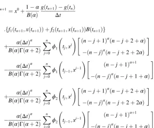
Fig. 1. Stochastic behavior of s(t).
Fig. 2. Stochastic behavior of ı(t).
Numerical simulation
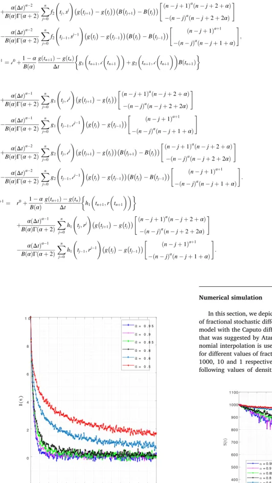
In this section, we depict numerical simulation of the chosen system of fractional stochastic differential equations. We have made use of the model with the Caputo differential operator and the numerical scheme that was suggested by Atangana and Toufik where the Lagrange poly-nomial interpolation is used. The numerical simulation are performed for different values of fractional orders. The used initial conditions are 1000, 10 and 1 respectively. The first 3 figures are depicted for the following values of densities of randomness 0.001, 0.006 and 0.006
Fig. 4. Stochastic behavior of ı(t). Fig. 5. Stochastic behavior of s(t).
+ α(Δt) α−2 B(α)Γ(α+2) ∑n j=0 f2 ( tj,sj ) ( g(tj+1 ) − g(tj ))( B(tj+1 ) − B(tj ))[(n − j + 1)α(n − j + 2 +α) − (n − j)α(n − j + 2 + 2α) ] − α(Δt) α−2 B(α)Γ(α+2) ∑n j=0 f2 ( tj− 1,sj− 1 ) ( g(tj ) − g(tj− 1 ))( B(tj ) − B(tj− 1 ))[ (n − j + 1)α+1 − (n − j)α(n − j + 1 +α) ] , in+1= i0+1 − α B(α) g(tn+1) − g(tn) Δt { g1 ( tn+1, i ( tn+1 )) +g2 ( tn+1, i ( tn+1 )) B(tn+1) } (137) + α(Δt) α−1 B(α)Γ(α+2) ∑n j=0 g1 ( tj, ij ) ( g(tj+1 ) − g(tj ))[(n − j + 1)α(n − j + 2 +α) − (n − j)α(n − j + 2 + 2α) ] − α(Δt) α−1 B(α)Γ(α+2) ∑n j=0 g1 ( tj− 1, ij− 1 ) ( g(tj ) − g(tj− 1 ))[ (n − j + 1)α+1 − (n − j)α(n − j + 1 +α) ] + α(Δt) α−2 B(α)Γ(α+2) ∑n j=0 g2 ( tj, ij ) ( g(tj+1 ) − g(tj ))( B(tj+1 ) − B(tj ))[(n − j + 1)α(n − j + 2 +α) − (n − j)α(n − j + 2 + 2α) ] − α(Δt) α−2 B(α)Γ(α+2) ∑n j=0 g2 ( tj− 1, ij− 1 ) ( g(tj ) − g(tj− 1 ))( B(tj ) − B(tj− 1 ))[ (n − j + 1)α+1 − (n − j)α(n − j + 1 +α) ] . rn+1= r0+1 − α B(α) g(tn+1) − g(tn) Δt { h1 ( tn+1,r ( tn+1 ))} + α(Δt) α−1 B(α)Γ(α+2) ∑n j=0 h1 ( tj,rj ) ( g(tj+1 ) − g(tj ))[(n − j + 1)α(n − j + 2 +α) − (n − j)α(n − j + 2 + 2α) ] − α(Δt) α−1 B(α)Γ(α+2) ∑n j=0 h1 ( tj− 1,rj− 1 ) ( g(tj ) − g(tj− 1 ))[ (n − j + 1)α+1 − (n − j)α(n − j + 1 +α) ] .
respectively. To obtain Fig. 4, 5 the densities of randomness used are given as 0.0016, 0.007 and 0.008, Figs. 7–9 0.0018, 0.01, and 0.01 finally figure Fig. 10–12, the randomness was removed. (See Fig. 6).
Conclusion
A simple SIR model was considered in this work. First we presented a detailed analysis of stability using existing technics such as Lyapunov function, the Ruth criteria. We presented the condition under which the Lyapunov function was positive, zero and negative. The system of or-dinary differential equation was converted to fractional stochastic dif-ferential equation with the aim to include into the mathematical model the effect of nonlocality and randomness. The existence and uniqueness has been presented. A numerical scheme based on the Lagrange inter-polation was used to solve numerically. Some simulations are presented.
Declaration of Competing Interest
The authors declare that they have no known competing financial
Fig. 6. Stochastic behavior of r(t).
Fig. 7. Stochastic behavior of ı(t).
Fig. 8. Stochastic behavior of s(t).
Fig. 9. Stochastic behavior of r(t).
Fig. 10. Stochastic behavior of s(t).
Fig. 11. Stochastic behavior of ı(t).