Menu optimization with large-scale data

(1)

MENU OPTIMIZATION WITH LARGE-SCALE DATA

JEYHUN KARIMOV

MASTER THESIS

THE DEPARTMENT OF COMPUTER ENGINEERING

TOBB UNIVERSITY OF ECONOMICS AND TECHNOLOGY THE GRADUATE SCHOOL OF NATURAL AND APPLIED

SCIENCES

DECEMBER 2015 ANKARA

(2)

Approval of the Graduate School of Natural and Applied Sciences.

Prof. Dr. Osman ERO ˘GUL Director

I certify that this thesis satisfies all the requirements as a thesis for the degree of Master of Science.

Prof. Dr. Murat Alanyalı Head of Department

This is to certify that we have read this thesis and that in our opinion it is fully adequate, in scope and quality, as a thesis for the degree of Master of Science.

Asst. Prof. Dr. Ahmet Murat ¨Ozbayoglu Supervisor

Examining Committee Members

Chair : Prof. Dr. Ali Aydın SELC¸ UK

Member : Asst. Prof. Dr. Ahmet Murat ¨Ozbayoglu

(3)

TEZ B˙ILD˙IR˙IM˙I

Tez i¸cindeki bütün bilgilerin etik davranı¸s ve akademik kurallar ¸cer¸cevesinde elde edilerek sunuldu˘gunu, ayrıca tez yazım kurallarına uygun olarak hazırlanan bu ¸calı¸smada orijinal olmayan her türlü kayna˘ga eksiksiz atıf yapıldı˘gını bildiririm.

I hereby declare that all the information provided in this thesis was obtained with rules of ethical and academic conduct. I also declare that I have sited all sources used in this document, which is written according to the thesis format of the Institute.

(4)

University : TOBB University of Economics and Technology Institute : Institute of Natural and Applied Sciences

Science Programme : Computer Engineering

Supervisor : Asst. Prof. Dr. Ahmet Murat ¨Ozbayoglu Degree Awarded and Date : M.Sc. – December 2015

Jeyhun KARIMOV

MENU OPTIMIZATION WITH LARGE-SCALE DATA

ABSTRACT

The use of optimal menu structuring for different customer profiles is essential because of usability, efficiency, and customer satisfaction. Especially in compet-itive industries such as banking, having optimal graphical user interface (GUI) is a must. Determining the optimal menu structure is generally accomplished through manual adjustment of the menu elements. However, such an approach is inherently flawed due to the overwhelming size of the optimization variables’ search space. We propose a solution consisting of two phases: grouping users and finding optimal menus for groups. In first part, we used H(EC)2 _{S , novel Hybrid}

Evolutionary Clustering with Empty Clustering Solution. For second part we used Mixed Integer Programming (MIP) framework to calculate optimal menu. We evaluated the performance gains on a dataset of actual ATM usage logs. The results show that the proposed optimization approach provides significant reduction in the average transaction completion time and the overall click count.

(5)

¨

Universitesi : TOBB Ekonomi ve Teknoloji Üniversitesi Enstitüsü : Fen Bilimleri

Anabilim Dalı : Bilgisayar M¨uhendisli˘gi

Tez Danı¸smanı : Asst. Prof. Dr. Ahmet Murat Özbayoglu Tez Türü ve Tarihi : Yüksek Lisans – December 2015

Jeyhun KARIMOV

B ÜY ÜK VER˙I ˙ILE MEN Ü EN˙IY˙ILEMES˙I

¨ OZET

Farklı mü¸steri profilleri i¸cin en uygun menü kullanımı kullanılabilirlik, verimlilik ve mü¸steri memnuniyeti a¸cısından esastır. Ozellikle bankacılık gibi rekabet¸ci¨ sektörlerde, en iyi menü kullanıcı arayüzüne sahip olmak bir zorunluluktur. Op-timal menü yapısının belirlenmesi genellikle menü elemanının manuel ayarlanması ile ger¸cekle¸stirilir. Ancak, bu metot özellikle kompleks menülerde i¸se yaramaz. Bu ¸calı¸smada iki a¸samadan olu¸san ¸cözüm önerilmi¸stir: kullanıcıları gruplandırmak ve gruplar i¸cin en uygun menüler bulmak. ˙Ilk bölüm i¸cin H(EC)2_{S, yeni hibrid}

Evrimsel Kümeleme algoritmasını geli¸stirdik. Ikinci bölümde optimal menü hesaplamak i¸cin Karı¸sık Tamsayılı Programlama kullandık. Sonu¸cları ger¸cek ATM logları üzerinde test ettik ve performans artımı oldu˘gunu gözlemledik.

(6)

ACKNOWLEDGEMENTS

I would like to thank my supervisor Asst. Prof. Dr. Ahmet Murat ¨Ozbayoglu, who gave me enormous, comprehensive support and high motivation to complete this thesis, conduct the complex research consisting of the implementation part, test, user study, survey and statistical analysis necessary for the thesis and a number of other research through my master degree period.

I thank Prof. Dr. Erdo˘gan Do˘gdu, Prof. Dr. Bulent Tavlı and Asst. Prof. Dr. Bu˘gra Ca¸skurlu for their contributions to my research.

My gratitude to TOBB University of Economics and Technology for providing me a scholarship throughout my study and to all staff members and assistants of the Computer Engineering Department of TOBB University of Economics and Technology for their deep teaching, advice, suggestions, which I appreciate the most.

I also thank Turkish Ministry of Science and Technology for their support provided as part of project No. 0.367.STZ.2013-2 and Provus Inc for providing me the data I used during my work.

(7)

LIST OF FIGURES

3.1 Execution overview of MapReduce . . . 8

3.2 Compact MapReduce programming model . . . 9

3.3 Intuition behind EFWA . . . 13

3.4 Improvement done on second part of k-means algorithm . . . 18

3.5 Demonstration of RC part . . . 24

3.6 Before CSC part . . . 27

3.7 After CSC part . . . 27

3.8 Intuition behind constructing new firework using graph. . . 28

3.9 Sample component design of web page . . . 31

3.10 Sample menu structure of ATM before optimization . . . 32

3.11 Sample menu structure of ATM after optimization. . . 33

3.12 Sample menu structure of ATM after optimization. . . 37

4.1 Comparison of three models in serial environment with DS-1. . . . 39

(11)

4.3 Comparison of three models in parallel w.r.t. data size. . . 41

4.4 Comparison of three models in w.r.t. node number. . . 42

4.5 Percentage of points changed in clusters in reduce step for k=5. . 44

4.6 Number of iterations before and after α = 0.15 threshold with DS-2. 45 4.7 Effect of k to fitness function. . . 46

4.8 Effect of increasing data size to execution time. . . 47

4.9 Effect of threshold level co on fitness value. . . 48

4.10 Effect of fireworks set size on fitness value. . . 48

4.11 Overall number of clicks with new model (NM) and previous model (PM). . . 50

4.12 Profile based comparison of number of clicks. . . 51

4.13 Average session time (in sec) on ATM with new model(NM) and previous model (PM). . . 52

4.14 Percentage of users used our model’s optimization menu items (SOP T). . . 52

(12)

LIST OF TABLES

3.1 Notations. . . 23 3.2 Terminology for MIP Formulations . . . 34

(13)

1. INTRODUCTION

Graphical User Interface (GUI) is the key point in multi-profile customer systems. Multi-profile customer systems can be considered as the systems that include many customers of different types. For example, web site, Automatic Teller Machine (ATM) or some phone app users can be divided to several types in terms of their behaviors or actions. The efficiency of menus in GUI can be calculated with click count, overall time, average time per transaction, and etc. to finish the required action. Are the existing menu structures are designed according to these requirements? Do they guarantee the optimum? These questions are important for both customers and industry. For example, customers can wait less time in ATM queues and companies can get customer satisfaction in return.

From initial perspective, menu optimization can be seen as a trivial problem. For example, finding the most clicked menu items and putting them to initial menu screens, is one solution. Moreover, when looking to menu items and their overall click counts, one can redesign the menu in a more optimized way. However, as menu structure gets complex we need deterministic solution, away from heuristics, guaranteeing the optimum. One important thing is that, any false assumption in heuristical based solutions can cost to companies to lose their customers.

Many researchers considered this problem to make better menus in GUI. Some solutions considered designing menu for people with disabilities [2, 3]. Yet in another solution ATM menus were designed based on questionnaires on customers [4]. All previous research we investigated, propose a menu model for GUI, based on some pre-assumptions. On the other hand, to be usable, the solution for optimal menu problem should be generic and applicable. For example, the solution should have no information about user types, their knowledge about system, the location of the system, questionnaires and etc. Moreover, the expected solution should be amorphous according to its application area and easily adjustable. For example, some company may need a menu with minimum click counts, other with minimum time, yet another with maximum menu item

(14)

size and visibility. Furthermore, usability is one of the main factors affecting the quality of software systems [5, 6, 7]. Therefore, the optimal menu has to ensure its usability. For example, the structure of menu cannot contain any disambiguous placement of menu items. So, the optimal menu is not just one solution but generic framework.

To design such a menu, we propose a 2-stage solution: clustering users and finding optimum solution for each group. For the first part, we developed a combined solution which encompasses fast and quality clustering within it. For the second part, mixed integer programming (MIP) framework is proposed.

The structure of this study is as follows. After this short introduction, we give literature review in Section 2. Then we provide a detailed explanation and solution of the problem in Section 3. Experiments are provided in Section 4. Possible applications of our model to various research areas and open research problems are given in Section 5. Our future work based on this method and conclusions are provided in Section 6.

(15)

2. RELATED WORK

There are various research conducted on clustering and GUI optimization. We grouped related works into categories.

2.1 Clustering

Because of its simplicity and applicability k-means [8] is the most widely used algorithm to cluster data. There are some studies implemented on optimizing different objectives of k-means algorithm such as Euclidean k-medians [9, 10] and geometric k-center [11]. Minimization of the sum of distances to the nearest center is the goal for Euclidean k-medians, and minimization of the maximum distance from every point to its nearest center is the one for geometric k-center version. Another research was done to seek a better objective function of k-means [12]. Although there are different versions of k-means that might have advantages, parallelization o the algorithm in a single machine resulted in significant performance improvement [13, 14]. Achieving the parallelization over multiple machines results in even better improvements. The MapReduce framework [1, 15] provides significant improvements to scalable algorithms. There has been several studies for clustering large scale data on distributed systems in parallel on Hadoop [16]. One such approach is Haloop [17], which is a modified version of the Hadoop making the task scheduler loop-aware and by adding various caching mechanisms. Another approach to cluster data in a distributed system was using Apache Mahout library [18]. Moreover, clustering of big data can be done on cloud also. In [19], the tests were running on Amazon EC2 instances and the comparisons were made to realize the gain between the nodes. Esteves et al. made comparisons over k-means and fuzzy c-means for clustering Wikipedia large scale data set [20]. Both in [20] and [19], the authors used Apache Mahout for clustering data.

(16)

2.2 Hierarchical Menu Optimization

Hierarchical menu optimization has been the main topic of many research works. In [21], authors developed an analytical model for search time in menus. The advantage of menu’s breath over its depth is stated in [22]. Researchers also showed experimentally that using broader and shallower menus instead of deeper and narrower ones make it easier and faster to access information [23, 24]. There are also hybrid solutions; in [25, 26] it is found that menus with larger breadth at deeper layers were more efficient than menus that became narrower towards the end. One of the earliest research conducted on menu optimization, [27], used the hierarchical index of a digital phone book using the access frequencies of phone numbers. Another approach is called ”split menus”[28] where frequently accessed menu items are located at the top of the menu groups or menu pages by splitting the menus. In [29], quantitive approach for hierarchical menu design was proposed by authors. Using Huffman Code to optimize the menu structure based on the probabilities of menu items’ access times is another approach that was proposed in [30].

2.3 Heuristic Solutions

There are some recent works that focus on using evolutionary algorithms and heuristics for menu optimization. Guided-Search algorithm is proposed in [31] for defining the necessary components of a good user interface. The authors of [32] used and tested the Guided-Search algorithm by analyzing the algorithm’s performance under different scenarios in order to increase the satisfaction level. Genetic algorithms were used for menu structure and color scheme selection in [33, 34] and in [35] authors used genetic algorithm with simulated annealing for optimizing the performance of menus on cell phones. Automated menu optimization and design is desirable but semantics always play a role. Therefore, some researchers suggested using human assistance as part of the optimization

(17)

and design process. In [36] authors present MenuOptimizer, a menu design tool that employs interactive optimisation approach to menu optimisation. The tool allows designers to choose good solutions and group items while delegating computational problems to an ant colony optimizer. [37] also suggests using informal judgements for the final menu structure along with an automated procedure.

Authors discuss GUI optimization techniques for evaluating and improving cell phone usability with efficient hierarchical menu design in [38]. Another research about cell phone menu optimizations, utilized menu option usage frequencies and recent usage history to find the best menu option ranking by using Ranking SVM method [39]. ClickSmart system was proposed in [40], to adapt WAP menus to mobile phones.

Fireworks algorithm, which was inspired by observing fireworks explosion, is a recent meta-heuristic that was proposed by Tan et al [41]. Authors showed that it outperforms Standard PSO and Clonal PSO in experiments. Enhanced Fireworks Algorithm is the improved version of the Fireworks algorithm [42], which we used in our model. Cuckoo search is another meta-heuristic that was proposed recently by Yang et al. [42], which was inspired by obligate brood parasitic behavior of some cuckoo species in combination with the Levy flight behavior of some birds and fruit flies.

2.4 ATM Menu Optimization

There have been several studies to optimize the menu structure on ATM [43, 44, 45, 46, 47] to reduce click counts and therefore waiting queues. The main objective is to display a menu that is optimal or results in less click counts to finish the required tasks for all users. Online banking user interface optimized with the same objective in [48]. Web site menu optimization is done with hill-climbing method which minimizes average time to reach target pages in [49].

(18)

Some works on GUI optimization make specific assumptions about users before optimization and optimize user menus accordingly. Authors emphasize the contributions of cognitive psychology and human factors research in the design of menu selection systems in [22]. In [50], authors concentrated on optimizing ATM menus for the usage of student communities. In [51] on the other hand, authors optimized ATM menus for illiterate people and tested on a group of six Dutch and functionally illiterate persons. Mobile interface GUI optimization was done for novice and low-literate customer usages in [52]. Designing ATM menus with speech-based and an icon-based interfaces for literate and semi-literate groups was conducted in [53]. In [54], authors reviewed a lot of different studies performed on Human Computer Interaction Technology for ATMs where they included different ATM design and implementations.

To the best of our knowledge, our solution is the first work on menu optimization which guarantees the optimum solution. In our generic GUI optimization framework in general and ATM menu optimization in particular, our solution is independent of any human assumptions, heuristics and other factors.

(19)

3. PROPOSED SYSTEM

We propose a solution which consists of two parts. To make better user menus it is crucial to cluster similar users and make menus for each cluster. In this way it is possible to get better performance and quality.

3.1 Clustering Part

3.1.1 MapReduce Framework

MapReduce is a programming model, mainly inspired by functional programming, used to process and generate large datasets with parallel and distributed algorithm on a cluster[1, 15]. MapReduce is useful in a wide range of applications, including distributed pattern-based searching, distributed sorting, web link-graph reversal, document clustering, machine learning[55]. MapReduce’s stable inputs and outputs are usually stored in a distributed file system. The transient data is usually stored on the local disk and fetched remotely by the reducers. The computational processing can occur on both unstructured and structured data. The programming model is as follows [1]:

• The computation takes a set of input key/value pairs, and produces a set of output key/value pairs.The user of the MapReduce library expresses the computation as two functions: Map and Reduce.

• Map, written by the user, takes an input pair and produces a set of intermediate key/value pairs: Map(k1,v1) → list(k2,v2).The MapReduce library groups together all intermediate values associated with the same intermediate key and passes them to the Reduce function.

• The Reduce function, also written by the user, accepts an intermediate key and a set of values for that key: Reduce(k2, list (v2)) → list(v3).

(20)

It merges together these values to form a possibly smaller set of values. Typically just zero or one output value is produced per Reduce invocation. The intermediate values are supplied to the user’s reduce function via an iterator. This allows us to handle the lists of values that are too large to fit in memory.

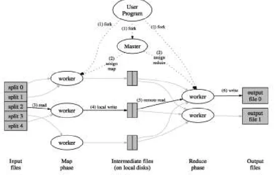
Figure 3.1 illustrates the MapReduce model Here the user program forks

Figure 3.1: Execution overview of MapReduce

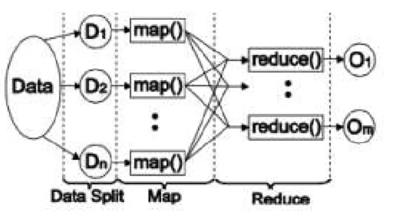
the process to all nodes. Then the master node assigns the roles and the responsibilities of mappers and reducers. After that, the input is splited into several partitions to be processed in parallel for mappers-workers. After all of the data is read, the map phase is finished. The input of the reducers is located on the local disks. Then the reduce phase begins and each reducer produces their output. More compact view of this model is shown in Figure 3.2

There has been several studies for clustering large scale data on distributed systems in parallel on Hadoop[16]. One such approach is Haloop[17], which is a modified version of the Hadoop MapReduce framework. The proposed model

(21)

Figure 3.2: Compact MapReduce programming model

dramatically improves the efficiency by making the task scheduler loop-aware and by adding various caching mechanisms. Authors used the k-means algorithm to evaluate their model against the traditional one and as a result, the proposed model reduced the query runtimes by 1.85.

Another approach to cluster data in a distributed system was using Apache Mahout library. Research was done to cluster data in the cloud [19]. The tests were running on Amazon EC2 instances and the comparisons were made to realize the gain between the node numbers. Yet another study was done to cluster Wikipedia’s latest articles with k-means [20].

Another research was concentrated on MapReduce model’s not directly support-ing processsupport-ing multiple related heterogeneous datasets [56]. Authors called their model Map-Reduce-Merge. It adds a Merge phase to the standard model. This phase can efficiently merge the data already partitioned and sorted by the map and reduce modules.

Meanwhile, working with large data sets in parallel and clustering them efficiently requires scalable and multi node computing machines. MapReduce architecture [1] is one particular example of such a system which had been in use more often lately. There are advantages of MapReduce over parallel databases like storage-system independence and fine-grain fault tolerance for large jobs[57].Because

(22)

MapReduce model works on multicore systems, there are some research done to evaluates the suitability of the this model for multi-core and multi-processor systems[58]. Authors of this research study Phoenix with multi-core and symmetric multiprocessor systems. Afterwards, they evaluate its performance potential and error recovery features. Moreover, they also compare the codes of MapReduce and P-threads which is written in lower-level API. As a result, authors conclude that MapReduce is a promising model for scalable performance on shared-memory systems with simple parallel code. MapReduce model is mostly used in offline jobs, because of its processing large data and late response time. However, authors of [59] researched the online version of Hadoop MapReduce framework.They propose a solution that allows users to see ’early returns’ from a job while it is being computed and process continuous queries on the framework.

3.1.2 k-means algorithm

k-means is one of the simplest unsupervised learning algorithms that attempts to solve the well known clustering problem[8]. In k-means clustering, we are given a set of n data points in d-dimensional space and an integer k and the problem is to determine a set of k points within n data points, called centers or centroids, so as to minimize the sum of mean squared distance from each data point to its nearest center. Initially, k centroids must be defined, one for each cluster. These centroids should be placed carefully because different location choices can result in different cluster formations. That is why, some heuristics suggest to place the centroids far away from each other as much as possible [60]. Afterwards, for each point that belongs to the given data set, it is associated with the nearest centroid. Then the new centroid is recalculated from the data points associated with each centroid. After calculating k new centroids, the algorithm must be iterated once again to find and associate each point to its nearest centroid. This loop continues as long as the locations of the new centroids keep changing until they all remain unchanged. The aim is to minimize the objective function given in (3.1)

(23)

J = k X j=1 n X i=1 x j i − cj 2 (3.1) where x j i − cj

is a distance measure between a data point x

j

i which is ithelement

of the data set n belonging to jth _{centroid ,and the cluster center c}

j. To wrap up,

the pseudo-code for the algorithm can be rewritten in this way:

1. Select k points in the space of objects being clustered. These points are initial centroids.

2. Calculate each object’s distance against all of the centroids and assign each object to the group that has the closest centroid

3. When all objects have been assigned, recalculate the positions of the k centroids by the formula:

cj+1 = 1 |Sj| n X i=1 xi (3.2)

where c is the new centroid,Sj is the number of x objects associated with

the jth _centroid

4. If any of the new centroids that was found in step 3 is different from the previous one, repeat Steps 2 and 3, else exit.

Time complexity of the k-means algorithm is O(mn) where n is the number of data points and m is the number of iterations. The number of iterations m tends to increase when the number of clusters (k) increases, however the number of data points that change their associated centroids tend to decrease during the consequent iterations, however the original k-means algorithm does not utilize this phenomena, i.e. the number of operations performed at every iteration is the same regardless of the number of data points that actually change their centroids. Authors used MapReduce framework to implement k-means in

(24)

parallel environment also[61]. One of the models we used to evaluate and compare proposed solutions was [61].

In this first part of the study, we propose a simple heuristic that is aimed to utilize the decreasing number of operations in these further iterations for k-means. We implemented the algorithm both serially and in parallel to evaluate how much efficiency is obtained under different scenarios.

3.1.3 Fireworks Algorithm

Enhanced Fireworks algorithm (EFWA) is a swarm intelligence algorithm and adopts four parts to solve optimization problems. The first part is the explosion operator. Suppose the population of EFWA consists of N D-dimensional vectors as individuals, each individual ’explodes’ according to the explosion operator and generates sparks around it. The second part is the mutation operator. Sparks are generated under the effect of this operator in order to improve the diversity of the population. The third part, namely as the mapping rule, is used to map the sparks that are out of the feasible space into it. By applying this rule, the sparks are pulled back to feasible space. The last part is called as selection strategy. The individuals are selected from the whole population and passed down to the next generation.

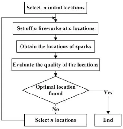
When a firework is set off, a shower of sparks will fill the local space around the firework. In our opinion, the explosion process of a firework can be viewed as a search in the local space around a specific point where the firework is set off through the sparks generated in the explosion. Mimicking the process of setting fireworks, a rough framework of the algorithm is depicted in Figure 3.3.

(25)

Figure 3.3: Intuition behind EFWA

3.1.4 Clustering Performance Improvement

k-means is the best known algorithm for clustering for its usability and scalability. Although there are numerous modifications of the k-means algorithm, both in single machine and in MapReduce model, the complexity of the algorithm more or less remains the same. In particular, Standard k-means (k-means-s) model can not escape from the complexity of the algorithm where the new centroids and nearest centroids are recalculated each time [61]. So, in each iteration:

• First part (P1) - All points are processed and the nearest centroids are found

• Second part (P2) - All points are processed in k groups to find the new centroids

(26)

As can be seen above, reprocessing of all points twice in each iteration increases the computation time of the algorithm linearly as the data and k value gets bigger. Improvement for the first part was done in [62]. However, this improvement have some disadvantages when working with big data. That is why, we further improved the model proposed in [62] and proposed two new solutions for the parallel computation with big data and the serial computation with non-big data. We will show the threshold between big data and non-big data for the data sets we used, in Section 4.

The models we propose, namely k-means-inbd (k-means improved for non-big data or k-means Improved for Serial Computation) and k-means-ibd (k-means improved for big data or k-means Improved for Parallel Computation), eliminates the majority of the complexity associated with both parts of the standard parallel k-means [61]. This improvement decreases the computation time and the complexity of the algorithm considerably. So, let

• xi denote a single data point and S denote all set of points in data set,where

xi ∈ S∀i.

• ct

j ∈ Ct denote the centroid computed in tth iteration, where j =

{1, 2, 3, ..., k} • St

j denote the set of data points belonging to ctj

• Pt

j denote the set of newly accepted points to cluster representing ctj

• Mt

j denote the set of outgoing points from cluster representing ctj

• zi denote the distance between xi and its belonging centroid.

• vi denote the index of xthi belonging centroid, ctk from the set Ct

• α be a constant value denoting threshold value where 0 < α < 1.

The first proposed model is k-means-inbd. General procedure of this model is as follows:

(27)

In the first iteration of k-means-inbd, for all data points, their nearest centroids are calculated and for each xi ∈ S , we keep zi and vi. After that, new centroids

are calculated as in k-means-s. Beginning from t = 2th_{iteration, when computing}

the nearest centroids for each data point, xi ∈ S, we calculate dt(xi ,ctvi), distance

between current data point and its previous centroid’s new value. That is, ct vi

is the newly computed value of centroid ct₋₁ vi . If d

t _{≤ z}

i, then xi stays in same

cluster. Thus, it can be ignored during the recalculation of the new centroid. Otherwise, it means that xi has changed its cluster and it must be considered

while recalculating the new centroids. After processing all data points, only those that were chosen are considered in the calculation of the new centroids. So, the calculation of a new centroid is shown with Formula (3.3):

ctj = ctj−1∗ |S t₋₁ j | − ( Pa i=1mti) + ( Pb i=1pti) |Sjt−1| − a + b (3.3) where ct

j ∈ Ct is the jth centroid among k centroids at tth iteration, |S t−1

j | is the

number of points belonging to ct₋₁

t , mti ∈ Mjt is ith point that is drawn out from

jth _{cluster at t}th _{iteration, p}t

i ∈ Pjt is ith point that is added to jth cluster at tth

iteration, b = P t j and a = M t j

. The pseudocode of k-means-inbd is shown in

Algorithm (1).

The second proposed model is k-means-ibd (k-means improved for big data). The general structure of algorithm is as follows:

• Before threshold part (BT ) - For i iterations until reaching threshold value, run as k-means-inbd. At each iteration t, compute threshold value αt.

• After threshold part (AT ) - if αt > α, then run Algorithm (3).

The first i iterations until reaching threshold value is as the same as k-means-inbd. Beginning from (i + 1)th _{iteration, we store centroids of previous iteration}

and size of all clusters. The iteration number i is decided as a result of threshold value α. That is, if the division of data points that changed their clusters to all

(28)

Algorithm 1

1: procedure k-means-inbd(xi ∈ S, ∀i , k)

Require:S = {x0, x1...xn}, k is number of clusters

Ensure: c1, c2, ..., ck centroids

2: Initialize centroids for t = 1.

3: Run k-means with its standard execution for the first iteration and keep

zi and vi ∀ xi ∈ S.

4: Initialize Ct_{, set of resulting centroids at the end of iteration t = 1.}

5: while ct j 6= c t₋₁ j ∀j do 6: t = t + 1. 7: for all xi ∈ S do 8: Compute distance dt_{= d(x} i, ctvi) and d t₋₁ _{= z} i. 9: if dt_{≤ d}t−1 _then _continue. 10: else 11: Compute ct

b ∈ Ct, xthi new associated centroid from set Ct, where b 6= j.

12: P_bt= P_btS

xi, add xi to set of new coming points for centroid ctb

13: Mt

j = Mjt

S

xi, add xi to the set of outgoing points for centroid ctj−1.

14: Save xth_i associated zi and vi, to use in the next iteration.

15: Compute the new centroids using Formula (3.3).

data points in tth _{iteration (α} t=

|Pt_|

|S| ) is less than predefined threshold (α), then we can be confident about clusters’ being mostly stable. Important point is that, after threshold value is satisfied, in AT part, we do not keep all points’ associating centroids, but the set of newly computed centroids, which can fit in memory in big data sets. In AT part, when recomputing the object assignments to the new centroids, the first to consider is the previous centroid. First we compute xth i

previous nearest centroid, ctj−1. When computing the new centroid, begin from

jth _{centroid from C}t_{, namely c}t

j. If dt−1(xi, cjt−1) ≥ dt(xi, ctj) , it means that the xi

stayed in the same cluster and there is no need to consider this data point when computing the new centroids. Otherwise, the data point has changed its cluster and it must be considered while recalculating a new centroid. Recalculating the new centroid part is the same as k-means-inbd. The pseudocode of k-means-ibd is shown in Algorithm (2).

(29)

Algorithm 2

1: procedure k-means-ibd(xi ∈ S, ∀i , k)

Require:S = {x0, x1...xn}, k is number of clusters

2: while αt> α do

3: Run Algorithm (1) for 1 iteration.

4: Compute αt=

|Pt_|

|S|, overall fraction of points that changed their existing clusters. Here |Pt_{| = |M}t_|

5: Run Algorithm (3) with required parameters from this algorithm.

Since we compared both the parallel and the serial versions of the proposed mod-els, MapReduce version of k-means-ibd and k-means-inbd was also implemented. The algorithm is the same. However, the mapping of the serial version’s first part (evaluating each data point’s nearest center) to the parallel version’s mapper phase and the serial version’s second part (calculating the new centroids after all data points chose their nearest centers) to the parallel version’s reducer phase is enhanced. That is, in the mapper phase we find the data point’s nearest centroid and in the reducer phase the new centroids are calculated from the points that changed their cluster.

3.1.4.1 Analysis of Proposed Models

When analyzing the proposed models, we can divide the means-inbd and k-means-ibd into two parts as k-means-s:

• First part - All points are processed and the nearest centroids are found. • Second part - All points are processed in k groups to find the new centroids.

Both k-means-inbd and k-means-ibd have improvements in the second part. If we examine Figure 3.4 which explains Formula (3.3), it can be seen that there are two main subparts denoted as 1 and 2. First, denoted as 1, is a computationally

(30)

Algorithm 3

1: procedure k-means-ibd-at(xi ∈ S, ∀i , k, Ct )

Require:S = {x0, x1...xn}, k is number of clusters, Ct set of

current centroids.

2: Initialize centroids for t = 1.

3: while ct

j 6= ctj−1 ∀j where 0 < j ≤ k do

4: t = t + 1.

5: for all xi ∈ S do

6: Among previous centroids, find the nearest centroid ct−1

j ∈ Ct−1 to

xi and compute distance between them dtj−1 = d(xi, ctj−1).

7: Find dt_j = d(xi, ctj), distance from xi to jth cluster from Ct, where j

is index of ctj−1. 8: if dt j ≤ d t₋₁ j then continue. 9: else 10: Compute ct

b ∈ Ct, xthi new associated centroid from set Ct, where

b 6= j.

11: Pt

b = Pbt

S

xi, add xi to set of new coming points that belong to

centroid ct b.

12: Mt

j = Mjt

S

xi, add xi o the set of outgoing points that belonged to

centroid ct₋₁ j .

13: Save only the set Ct _{to be used in the next iteration.}

14: Compute the new centroids using Formula (3.3).

constant time operation. As we will discuss in the experimental results, it is seen that second part, denoted as 2, consists of a small minority of the points of the whole data set, so as the iterations progress, the number of operations keep decreasing geometrically, i.e. the total number of operations converges to a constant; hence the whole formula can become a constant time operation.

Figure 3.4: Improvement done on second part of k-means algorithm While analyzing the first part of proposed models, in k-means-ibd model, we are interested in minimizing the overall data sent from mapper to reducer phase and minimizing I/O time. The main advantage of k-means-ibd is that, it does not

(31)

change the original data after threshold is satisfied. So, there is no disc-write overhead, in any iteration after αt < α. Important point here is that, after

threshold value is satisfied, overall points tend to stay in their existing clusters, as we will see in Section 4. Therefore, we switch to Algorithm (3). This algorithm keeps only the previous centroids set which can be kept in the memory for very large data sets. That is why, as the size of the data gets bigger, k-means-ibd starts outperforming inbd in MapReduce parallel computing model. k-means-inbd on the other hand, has less complexity compared to k-means-ibd. Because k-means-inbd model keeps all data points’ previous centroids, after several steps, calculation of the new centroids is taking O(1) instead of O(k) time most of the time. However k-means-inbd has an obvious space disadvantage. That is, when working with big data, in every iteration, all data points’ centroids must be read and written to the disc, since they can not be kept in the memory. As it will be seen in Section 4, there is threshold value for data set depending on the overhead of writing big data to disc that dominates over k-means-inbd’s improvement in the first part of the algorithm. That is why, we considered this algorithm to be the best for the serial implementation and for the parallel implementation with upper bound data size.

As demonstrated in [63], the worst-case running time of k-means is superpolyno-mial by improving the best known lower bound from Ω(n) iterations to 2Ω(√n)_.

That is, k-means always has an upper bound, therefore it always converges. So, because it always converges, the displacement speed of centroids must go to zero as iterations go to some finite number. Therefore, their speed must decrease, otherwise the algorithm cannot converge. Because centroids’ speed decrease, the points that belong to particular centroid, tend to stay in that cluster.

3.1.5 Clustering Quality Improvement

Even though k-means is not the best performing data clustering algorithm, it is still by far the most widely-used one due to its simplicity, scalability and

(32)

convergence speed. However, depending on the initial starting centroid points, significantly different results can be obtained, so the algorithm is highly sensitive to its random centroid selection.

Meanwhile there is also another notable problem with k-means algorithm. When the number of cluster formations increase, the possibility of obtaining empty clusters (locations that do not have any data points associated with the clusters) also increases at each iteration. This becomes an unavoidable issue when k >> 1. This issue was not addressed thoroughly in most of the studies.

In this study we not only aim to improve the clustering quality of k-means, but also provide a methodology that can overcome ”empty clustering” problem without jeopardizing the convergence speed, so the proposed model could be used for all clustering problems regardless of the number of data points, number of data dimensions and number of clusters. We achieved this by using an initial centroid selection algorithm based on a hybrid model that is a combination of evolutionary algorithms (Fireworks and Cuckoo search) and some additional heuristics. Our model, H(EC)2_{S, Hybrid Evolutionary Clustering with Empty Clustering}

Solution, consists of 4 parts: Representative Construction (RC) part, Enhanced Fireworks algorithm for Clustering (EFC) part, Cuckoo Search for Clustering (CSC) part and k-means part. Firstly, instance reduction is done to select representatives for existing data. This part does the main job to eliminate Empty Clustering problem, because in latter parts, the centroids are selected among representative points only. Secondly, in EFC part, the solution space is searched using Enhanced Fireworks algorithm. Thirdly, in CSC part, we construct new solutions and based on Cuckoo Search algorithm, place solutions to ”host nests”. Finally, we pass the selected best firework to the k-means and converge. The pseudo-code of the proposed model is given in Algorithm 5. Some notations are given in Table 3.1.

(33)

3.1.5.1 RC Part

The main purpose of RC part is to select ”representative” instances among data which eliminate the instance count significantly. The important point is that, in RC part we can detect outliers and eliminate them also. Algorithm 4 shows the pseudo-code of RC-part. Lines 3-8 show the process of discretizing the values to find how many distinct data point there are at each dimension. Here si[j]

denotes the jth _{dimension value of i}th _{data point. Equation 3.16 maps each data}

point to a representative value, where mini and maxi represent min and max

elements at ith _{dimension respectively. To do this, it divides dimension range}

into Fi and finds in which portion the data is. Lines 9-13 find the representative

values rV alue for each data point. Lines 13-16 show the elimination part of representatives. That is, if the number of belonging data points are less than the specified threshold, co, then the data points can be considered as outliers and

representative can be deleted. Else, we find the average of all its belonging data points in each dimension and update the representative value. Finally, lines-17-20 show the case where the number of representative values do not fit into the memory, they are more than predefined threshold. In this case we either select another f function which is ”more” decreasing or increase cf or do both.

Algorithm 4 shows the main intuition behind RC part, which be can easily converted to MapReduce algorithm. That is, first we calculate distinct values in Mapper and send them to Reducers so that it can combine all distinct values in each dimension. Secondly, in Mapper we find each point’s representative and send it to Reducer with the point itself. Reducer gets the representative and its points and calculates the average of the points. Figure 3.5 shows the overall intuition over the RC part, where romb-like rectangles are representatives and black points are data.

(34)

Algorithm 4 RC-Part Require: si ∈ S data points

1: Let Hk be the HashMap related with kth dimension of data points, where

k = {1, 2...cd}

2: Ak be a vector, denoting the count of distinct values in kth dimension,

where k = {1, 2...cd}

3: for all si ∈ S do:

4: for j = 1 to cd do:

5: xi[j] ← Round si[j] to cf decimal places.

6: Put Hj a new entry with key=xi, value=1. If already exists, increment

value.

7: Ai ← P ej∈Hi

ej.value, ∀(i = {1, 2, ...cd})

8: Fi ← f (Ai)∀(i = {1, 2, ...cd})

9: for all si ∈ S do:

10: Compute rIDk _{k = 1, 2, ..c}

d using Equation 3.16

11: Rid ← Rid ∪ rID

12: D(rID) ← D(rID)∪ si

13: for all rIDi ∈ Rid do:

14: if ||D(rIDi)|| ≤ co then

15: Data points belonging to representative rIDi are outliers, so eliminate

rIDi 16: else rV aluek i ← P sj ∈D(rID_i) sj[k] ||D(rIDi)|| , ∀k = 1, 2, ...cd

17: if representatives are higher than predefined threshold (do not fit in memory) then 18: f () ← f (f ()) 19: Increase cf 20: Restart algorithm Algorithm 5 H(EC)2_S 1: Run RC part

2: for t = 1 to itermax do:

3: Run EFC 4: Run CSC

(35)

Table 3.1: Notations. rIDk

i ∈

Rid

The ID of ith _{representative data point, possibly int values}

denoting the range index, where k denotes dimension rV aluek

i ∈

Rvalue

The actual value of ith _{representative data point, where k}

denotes dimension

f : R → R Decreasing function from real numbers to real numbers cf Constant denoting how many decimal places should data be

rounded

maxd Maximum data point in dth dimension

mind Minimum data point in dth dimension

Ni Number of distinct data points in ith dimension

Fi Number of distinct data points in ithdimension after applying

f function to Ni

cd Dimension size of a data point

co Threshold value for ”representative” values to be used in

outlier detection. D(rID) or

D(rV alue)

Set of belonging data points to representative rID or rV alue E[i][j][n][k] Similarity matrix, that shows the shared data points count between ith _{firework’s j}th _{cluster and n}th _{firework’s k}th_cluster

f wji ∈ F Firework (a possible solution) of index i in set F , where k is

the centroid of firework.

(36)

Figure 3.5: Demonstration of RC part

3.1.5.2 EFC Part

In this part, we use Enhanced Firework Algorithm (EFW) to search the solution space for ”good” initial points. Initially, the model starts with random solution, converts it to representative using Equation 3.16 and calculates amplitude and and sparks locations. The sj[i] represents ith dimension value for some sj ∈

S, mini and maxi are minimum and maximum values in ith dimension. After

that, while computing their fitness values, it also derives 4 dimensional similarity matrix E. The important point is that, we use the reduced data set with only representatives for selecting centroids, Rvalue, derived in RC part. Then, we find

the amplitude and spark sizes in each dimension of firework and update fireworks. After updating, we convert them to representative values with Equation 3.16. The pseudo-code for this part is given in Algorithm 6.

The construction of firework f w as a solution is done via concatenating the k centroids. That is, because we seek a solution of k centroids to cluster data, we represent the solution, f w, as a combination of k cluster centroids. Equation 3.11 controls the Ak

(37)

initially to explore the solution space and diminishes gradually. Here t refers the number of function evaluation at the beginning of the current iteration, and evalsmax is the maximum number of evaluations. Ainit and Af inal are the initial

and final minimum explosion amplitude, respectively. Equation 3.12 controls the amplitude so that it does not become too small. Equation 3.13 calculates the value of amplitude, where g is fitness function, ymax = max(g(Xi)) and

ymin = min(g(Xi)) are the two constants to control the explosion amplitude

and the number of explosion sparks, respectively, and ǫ is the machine epsilon. Equation 3.14 calculates the number of sparks.

Algorithm 6 EFC-part

1: Initialize random fireworks f wi ∈ F

2: Calculate fitness of each firework f ti ∈ F T using Equation 3.15, where M

is positive constant, sji is jth dimension value of si and cj is jth centroid

which sji belong to. While doing this, update the value of E array,

such that, if data point belongs to f wk

i and f wjm then, E[i][k][j][m] ←

E[i][k][j][m] + 1

3: Calculate si, the number of explosions for each firework using Equation

3.14

4: Calculate Ai for every firework using Equation 3.13, 3.12 and 3.11

5: for all f wi in F do:

6: for j = 1 to si do:

7: ∆X_ik ← round(rand(0, 1)) ∗ Ai∗ rand(−1, 1)∀(k), calculate displacement,

where 1 ≤ k ≤ K is cluster count

8: if Xk

i is out of bounds then

9: X_ik ← X_mink + |X_ik|%(X_maxk − X_mink ) 10: Xk

i ← Xik+ ∆Xik ∀(1 ≤ k ≤ K)

11: Perform k-means and update E array

12: Calculate fitness values of fireworks f wi ∈ F using Equation 3.15

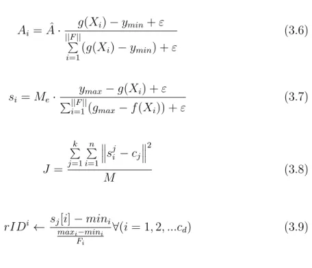
Ak_min(t) = Ainit− Ainit− Af inal evalsmax q (2 ∗ evalsmax− t)t (3.4) Aki =      Ak min if Aki < Akmin, Ak i otherwise. (3.5)

(38)

Ai = ˆA · g(Xi) − ymin+ ε ||F || P i=1(g(Xi) − ymin) + ε (3.6) si = Me· ymax− g(Xi) + ε P||F || i=1(gmax− f (Xi)) + ε (3.7) J = k P j=1 n P i=1 s j i − cj 2 M (3.8)

rIDi ← sj_max[i] − min_i_−min_i i

Fi

∀(i = 1, 2, ...cd) (3.9)

3.1.5.3 CSC Part

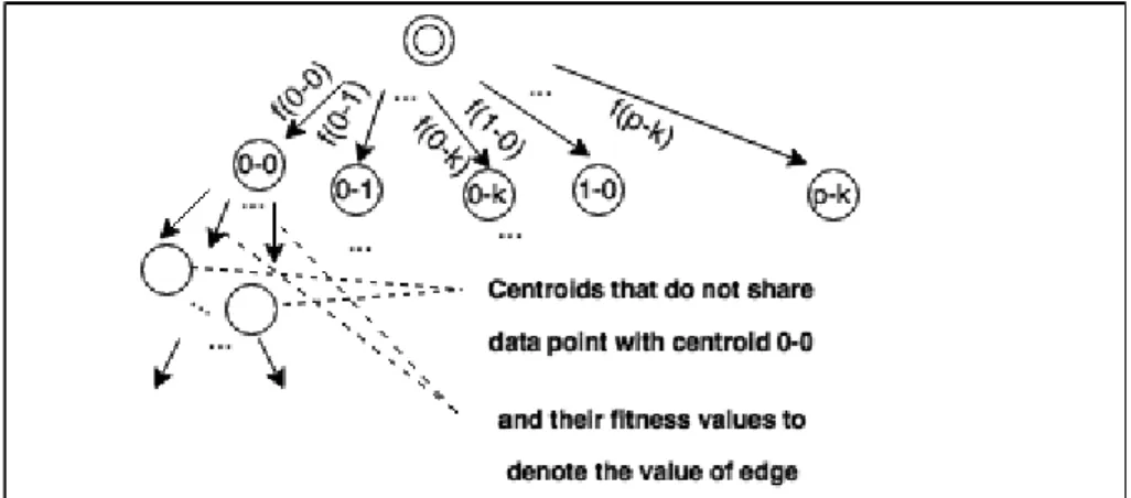
In this part, new fireworks are constructed and joined to firework set. We use E, 4 dimensional array to construct new solutions and use Cuckoo Search algorithm to select fireworks in F to pass to the next generation. To construct the new fireworks, k different centroids from different fireworks are found and joined. The important point is that, k different centroids cannot share any data points, because in a particle centroids do not have any common data points.

For example, Figures 3.6 and 3.7 show the procedure of creating new firework with k=3 and ||F ||=2. Figure 3.6 and Figure 3.7 are before-after situations of constructing new firework. In Figure 3.6, one firework is denoted with rectangle and another with triangle. CSC computes that centroids denoted with 0 − 0 , 1 − 1 and 0 − 1 do not share any common data points,where f − k means kth

centroid of fth _{firework. As a result, the new particle can be created as shown in}

Figure 3.7 with plus sign. Indeed, if this was a separate particle, it would have better fitness value than the existing ones.

(39)

Figure 3.6: Before CSC part

Figure 3.7: After CSC part

We use the similarity array E to form a graph consisting of vertices denoted with centroids and edges having value of that vertex’s fitness value. Since the similarity array keeps the sharing data point count between centroids, if the shared element count is zero, then the corresponding centroids can be concatenated to form a new firework. As can be seen from Figure 3.8, the source node is the double lined circle. It has ||F || ∗ K child nodes, since that is precisely the total number of centroids within the firework set. The source node do not share any points with any of the centroids. As a result, some path, with the minimum sum of edge values, consisting of K consecutive nodes is found, where the incoming edge value of a particular node is its fitness value. Important point is that, the K consecutive nodes can be anywhere in the graph, might not necessarily begin

(40)

from the source node. To solve this problem, dynamic programming is used and all possibilities are tried like brute force, but in a ”careful” way.

DP (k, ck p) = argmin(DP (k − 1, n k p) + f k p, DP (k, n k p))∀(n k p) (3.10)

As can be seen from Equation (3.10), finding the minimum length k united nodes is implemented recursively, where nk

p is the child node of ckp. The number of

nodes needed and the current node are the two arguments given to function DP . Finding the minimum path length consisting of k nodes can be done by either taking the current node into consideration, running the same function for the rest of its child nodes with (k − 1) needed nodes and summing them, or not taking the current node into the consideration and running the function with K and all of current node’s child nodes arguments, and giving the minimum of this results as an output. We used memoization in order to get the advantages of dynamic programming. That is, if some value of DP (k, nk

p) = c then it is stored, and after

if it is needed, then the answer is retrieved in constant time and used.

After finding new solutions we use Cuckoo Search to place them. The pseudo-code for Cuckoo search is given in Algorithm 7.

(41)

Algorithm 7 CSC-part

1: Calculate objective functions fobj(f wi)∀f wi ∈ F with Equation 3.15.

2: Get ni ∈ N new firework solutions with Equation 3.10

3: for i = 0 to itermax do

4: Chose random ni

5: Chose random fi

6: if fobj(ni) isbetterthan fobj(f wi) then

7: Replace f wi by ni with some probability

8: Delete pa fraction of F and build new fireworks randomly.

3.2 Optimization Part

Having clustered users, it is essential to construct a menu for each of the groups. The reason that we cluster users first is that to group them into similar clusters which can lead to better menus for each group. Obviously, it is not possible to make better menu for all users. Therefore, grouping them and making optimal menu for each group leads to better performance.

To explain overall system, we first present the problem definition with possible input and output constraints and optimization framework.

3.2.1 Before Optimization

Optimizing menu for specific needs is a challenge because it is vital to have understandable and usable menu after optimization part. There are some input and output specifications to be cleared before constructing a model. The steps that we have done before optimization, including in Clustering part:

• Mine user logs. The logs of user transactions have to be mined and for each user its corresponding customer profile must be derived.

• Cluster users. That was the process we have done in first part of solution. • Derive menu tree. Here the menu screens can be thought as tree vertices

(42)

and relations between screens are edges in tree. For example, in Figure 3.9, the sample menu tree of some website is shown.

• Define optimization objective. For example, minimizing click count, maximizing menu visibility, minimizing overall session time and etc. can be objective for menu optimization. In this study we focused on minimizing click count problem.

• Calculate click counts for each menu screen for each cluster. The click count of each menu screen is not calculated as the number of clicks for particular menu item. Instead, our objective is to get actual aim of user. For example, if user clicks menu A then B and then C, and stays in A and B negligible time, then his/her aim is to reach menu C. So, counting menus A and B for this aim is worthless. Therefore it can be the case that the menu item under other menu item can have high click count than its ”parent” menu. • Put click counts on tree nodes for each cluster. In menu tree, we put click

count of each menu screen to its relative vertex. That is, the value on the vertex corresponding to particular menu screen, is equal to that menu screen’s click count.

Having input specifications our aim is :

• Construct a menu tree out of existing one such that the overall click count is minimized. For example, if menu C is under menu B and menu B is under menu A (A→B→C), and if menu C is very usable (having high click count), then to reach this menu users click more. If we reposition menu C is nearer position to main menu (A), then overall click count can be minimized. • Ensure the usability and understandability. To reconstruct the menu in

optimum way, one can say that using Huffman coding [64] and placing the most clicked menu on top and reconstructing all subtree in this manner gives the best solution. This is true but how about usability? For example, we have in original menu structure ”Fox”,”Cat” and ”Elephant” is under

(43)

Figure 3.9: Sample component design of web page

the ”Animal” menu. If ”Cat” is clicked much more than others, we cannot be put ”Cat” on top of ”Animal” menu, because this would mislead the users and affect usability negatively.

• Ensure the additional constraints. Some devices can have constraints such as maximum menu buttons for each page. For example, in phone or ATM menus the space constraints are important issue. Our model handles it considering each menu screen’s maximum children menu pages.

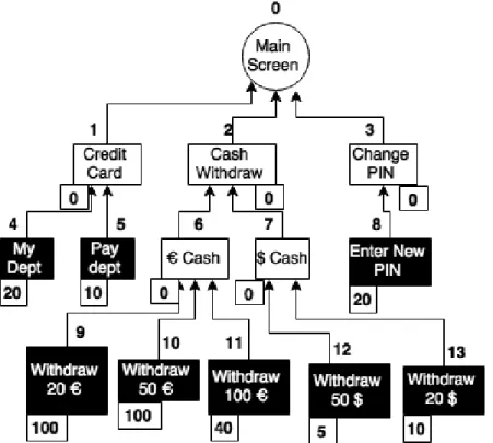
Figure 3.10 gives sample menu structure of ATM, where rectangle boxes represent menu item, the numbers above boxes represent their ID, the ones below boxes represent click counts for particular menu item and black boxes represent ”leaf” menu items, meaning last menu item in the click path. Moreover, we assume that the menu shown in Figure 3.10 can have at most 3 children per node.

(44)

The optimal version of that menu based on the click count is given in Figure 3.11. It is clear that, the menu is optimum when it conserves both usability and understandability. Meanwhile, in this particular case, finding the optimal menu for Figure 3.10 is not very hard. However, considering very large menus for complicated systems or enormous networks, the optimization is not an easy task.

Figure 3.10: Sample menu structure of ATM before optimization

3.2.2 Optimization Framework

To optimize user menus we assume that, the user logs are mined in an efficient way, they are clustered and click counts of menu items for each cluster is known. Using MIP framework we guarantee the optimum. The key concepts are represented in Table 4.1 and in Figure 3.12. In this solution, we represent the menu as tree and show the existing problem as a network flow problem. The flow generated in each node is equal to overall click count on particular node and aim

(45)

Figure 3.11: Sample menu structure of ATM after optimization.

is to minimize the overall flow. Figure 3.12 shows the original menu and dashed lines represent possible connections between nodes that can be selected while optimization. As can be seen from Figure 3.12, we introduce 2 new node types: optimizers (triangle-like boxes) and combiners (romb-like boxes). The details and their usage is given below:

• Optimizers - These are menu nodes introduced in this study to bring best leaf node or menu subtree to upper levels. That is, the optimizer has possible connections to all ”grandchildren” nodes of its parent, but selects only out of them. For example, in Figure 3.12, nodes with ID=14,17 and 18 are optimizers and all lower level nodes with same parent (Main Screen) are connected to them. The optimizer selects the best option as there can be only one child for each of optimizers. Optimizers can have in all levels of a menu tree but the leaf level. For simplicity, in Figure 3.12, we put them only in the first level. The important point is that, optimizers can connect to not all low level menu nodes but only same-parent menu nodes with itself. Moreover, the cost of connecting to optimizer is zero. This constraint is put to encourage nodes to go to upper levels with minimum cost and the

(46)

Table 3.2: Terminology for MIP Formulations Variable Description

S (Given) Set of all original menu nodes, excluding optimizers and combiners.

SOP T(Given) Set of Optimizer menu items (triangles in Figure 3.12)

S0(Given) The root or top level menu item. (Node with ID=0 in Figure

3.12)

SCOM B(Given) Set of Combiner menu items, the ones shown with romb in

Figure 3.12)

Ci(Given) Integer that shows click count for ith node.

INi (Given) Set of candidate incoming nodes to ith node.

OU Ti (Given) Set of candidate outgoing nodes from ith node

Li

IN(Given) Constant number that shows the number of child nodes of ith

menu node. This number is maximum number of incoming nodes to ith _node.

Li

OU T (Given) Constant number that shows the number of parent nodes of ith

menu node. This number is the maximum allowed number of outgoing nodes from a particular node i.

fij(Variable) Amount of flow (click in this case) between menu nodes i and j

aij(Variable) Boolean variable which denotes if there exist a flow between the

nodes i and j

dij(Given) Integer value denoting the weights of arcs. In general, all weights

are equal to one, but the ones incoming to SOP T are equal to 0

M (Given) Large constant with respect to given parameters in problem.

optimizer will select the best option to minimize overall system’s cost. • Combiners - These are menu nodes introduced in this study to combine

same level nodes under one menu node and take them one level below. For example, node with ID 16 is combiner. All same level nodes are possible child nodes of combiner. The main point is that, if some nodes in the same level are chosen to go downwards, they are collected under the combiner node with name like ”Others” and their previous places are taken by another menu nodes from downwards.

(47)

It is assumed that whatever the size of menu is, we have quite powerful machine to compute its optimum form. The model consists of several linear equations given below: aij ∈ {0, 1} ∀i ∈ S, ∀j ∈ OU Ti (3.11) fij ≥ 0 ∀i ∈ S, ∀j ∈ OU Ti (3.12) X j_∈OUTi fij − X j_∈INi fji =      −P i∈S−S0Ci, i = S0 Ci, ∀i ∈ S − S0 (3.13) fij ≤ M aij, ∀i ∈ S, j ∈ OU Ti (3.14) X j_∈OUTi aij      ≤ 1, ∀i ∈ SOP T ∪ SCOM B = Li OU T, otherwise (3.15) dij =      0, if j ∈ SOP T 1, otherwise ∀i ∈ S, ∀j ∈ OU Ti (3.16) X j∈INi aji      ≤ 1, ∀i ∈ SOP T ≤ Li IN, otherwise (3.17) Minimize : X j∈OUTi dijfij∀i ∈ S (3.18)

Equation 3.11 shows that aij is a boolean variable for all possible arcs defined in

(48)

Here, flow is the click count of a particular node. Equation 3.13 provides the flow balance in the system. There can be 2 separate cases. If the node is a sink node, that is, the one at the top level, then all incoming flow is equal to the sum of all flows generated in other nodes, since flows are made from clicks. Otherwise, the flow generated in particular node is the difference between incoming and outgoing flows. In equation 3.14, we are converting flows to binary variables to be used in later equations. Equation 3.15 shows the constraint related with outer arcs from a particular node. That is, there must be exactly Li

OU T number of arcs going out

of ith _{node, if the menu node is neither S}

OP T, nor SCOM B. This means that, a

particular node in the menu must be connected to the menu and it cannot be lost even it has no clicks. But in the case of SOP T and SCOM B nodes, they are free

to be connected to the tree or not. We are not forcing them to do so. Equation 3.16 shows the constant dij, which represents the weights of arcs. We say that

every arc in a tree has an equal weight of 1, except the ones incoming to SOP T

menu nodes. Since we want to encourage other nodes to connect to these nodes, their weights are 0. Equation 3.17 does the same for constraining the number of incoming arcs to a particular menu node. This can be thought as the maximum number of menu items under a particular menu item. We constrained SOP T’s

incoming nodes to maximum 1 node, as we are allocating SOP T nodes itself and

taking more than one incoming node would not optimize the system efficiently. Equation 3.18 shows our objective function. This is simply the minimization of flows multiplied by the arc weights. This can also be considered as the cost of a flow.

The important point is that, our model does not enforce using combiners and optimizers. If it is optimal, the system uses them in some or all levels of the menu tree. Another important point to mention is that, the click count of non-leaf nodes is not computed as regular. For example, there can be the case that, for one menu node m1 click count is c1, and for another menu node m2click count

is c2, where c2 > c1 and m2 is child node of m1. Here, for non-leaf menu nodes, we

do not compute click count as regular. If the user stays at a particular menu item for longer than some threshold time, then we add click count for that particular

(49)

menu node, else we consider that user’s purpose was not actually looking for this page; therefore, we do not add click count.

(50)

4. EXPERIMENTS AND ANALYSIS

Because our solution is multi-objective, we grouped the experiments from general to specific to menu optimization. Firstly, the clustering performance improvement experiments are presented. Then clustering quality improvement experiments are presented. Finally, considering clustering results are ready, we optimize menu structure and show results.

4.1 Experiments on Clustering Performance

Improvements

The experiments were conducted both in serial and parallel environment. MapReduce framework of Cloudera’s Apache Hadoop distribution was used for parallel environment. The environment consisted of 17 connected computers with 100M bit/s Ethernet. Each computer had Intel i7 CPU and 4GB RAM capacity. Among the 17 computers, 16 of them were worker nodes and 1 was the master node.

Two different data sets were used to run the experiments. First data set (DS-1) was, “Individual household electric power consumption Data Set” 1 _{and the}

second one (DS-2) was, “US Census Data (1990) Data Set” 2_{. The lengths of}

feature vectors of DS-1 and DS-2 are 7 and 68 and the size of data sets are 2075259 and 2458285 instances respectively. Both data sets were divided into different number of clusters and the algorithms run with different initial centroids. Finally, we chose α threshold to be 0.15 in experiments.

We have performed numerous experiments both in serial and parallel environ-ments. We compared our proposed improvements with the models proposed in

1 _{https://archive.ics.uci.edu/ml/machine-learning-databases/00235/}

(51)

[62], [65] and standard k-means - (k-means-s) [61]. The complexity and efficiency of the models described in [62] and [65] are mainly the same. Therefore we implemented the model shown in [62] to compare with our proposed algorithms. As the authors of [62] called their model as enhanced k-means, for simplicity we called their model as k-means-e.

Before discussing the results, one important thing is that, there is no k-means-s in figures, because the graphs show relative results with respect to k-means-s. Since in all of the fore-mentioned models we are trying to achieve improvements over k-means-s, all graphs shown in this section used k-means-s performance as the basis. This is accomplished by dividing the result of the particular model running time by the running time of k-means-s. This can also be considered as a normalization.

Figure 4.1: Comparison of three models in serial environment with DS-1.

Figure 4.1 shows the comparison of our proposed models and k-means-e [62] in terms of their efficiency towards k-means-s [61] with DS-1 in the serial environment. It is clear that k-means-ibd is less efficient compared to the other two models. As stated above, all proposed models consist of two parts: first part and second part. Here k-means-ibd mainly takes advantage of the improvement

(52)

Figure 4.2: Comparison of three models in serial environment with DS-2.

of the second part when compared to k-means-s. k-means-e also takes advantage of the improvement of the first part, when finding the nearest centroids. However, k-means-inbd is improved both in the first and the second part, that is why, it performs better than the other models. In general, it is obvious that when the data is small compared to the memory size and in the serial environment, first part of the models dominates the second part. That is why, even though k-means-ibd performs better than k-means-s, it is still slower than the other two models.

Figure 4.2 shows the same procedure as Figure 4.1 with DS-2. It is clearly seen that the overall concept is pretty much the same. Meanwhile, all models more or less have improved their performance slightly by decreasing their computation time. This is due to the fact that the feature vector size in DS-2 was 68, whereas it was 7 in DS-1. However, k-means-inbd and k-means-e improved their computation time more than k-means-ibd, when compared to Figure 4.1 because k-means-e and k-means-inbd benefit computationally over k-means-s in part-1 which is directly related to the vector size, more than k-means-ibd. As the vector

(53)

dimension increases, means-inbd and means-e have more dominance over k-means-s, since the first part of the proposed models have dominance over the second part in the serial environment.

The performance improvement over standard k-means increases with larger k values due to the increase in the number of iterations to converge, as seen in Figures 4.1 and 4.2. As the number of iterations increase, we have much more benefit using our proposed models compared to standard k-means.

Figure 4.3: Comparison of three models in parallel w.r.t. data size.

Figure 4.3 shows the comparison of the proposed models over k-means-s in the parallel environment. We used Cloudera’s Hadoop distribution with 17 nodes in this experiment. The main purpose of this experiment was to find the threshold value for the size of the data set where means-ibd starts outperforming k-means-inbd. Therefore we simulated DS-1 to have a larger data set. As stated during the analysis of the algorithms, the main disadvantage of k-means-e and k-means-inbd is their necessity to keep all data points’ previous centroids. If the serial environment is used with a data size that is less than the memory size, they can be kept in the memory. However with the increasing data size, it will not be possible to achieve that. In MapReduce implementation, k-means-e