YAŞAR UNIVERSITY
GRADUATE SCHOOL OF NATURAL AND APPLIED SCIENCES MASTER THESIS
AN ADAPTIVE LARGE NEIGHBORHOOD SEARCH
ALGORITHM FOR THE HETEROGENEOUS PICK-UP
AND DELIVERY VEHICLE ROUTING PROBLEM
WITH TIME WINDOWS
Gökberk Özsakallı
Thesis Advisor: Assoc. Prof. Dr. Deniz TÜRSEL ELİİYİ
Department of Industrial Engineering Presentation Date: 10.06.2016
Bornova-İZMİR 2016
ii
I certify that I have read this thesis and that in my opinion it is fully adequate, in scope and in quality, as a dissertation for the degree of master of science.
Assoc. Prof. Dr. Deniz TÜRSEL ELİİYİ (Supervisor)
I certify that I have read this thesis and that in my opinion it is fully adequate, in scope and in quality, as a dissertation for the degree of master of science.
Assoc. Prof. Dr. Pınar MIZRAK ÖZFIRAT
I certify that I have read this thesis and that in my opinion it is fully adequate, in scope and in quality, as a dissertation for the degree of master of science.
Assist. Prof. Dr. Erdinç ÖNER
--- Prof. Dr. Cüneyt GÜZELİŞ Director of the Graduate School
iii
ABSTRACT
AN ADAPTIVE LARGE NEIGHBORHOOD SEARCH ALGORITHM FOR THE HETEROGENEOUS PICK-UP AND DELIVERY VEHICLE
ROUTING PROBLEM WITH TIME WINDOWS
Özsakallı, Gökberk MSc in Industrial Engineering
Supervisor: Assoc. Prof. Dr. Deniz TÜRSEL ELİİYİ June 2016, 69 pages
In this thesis, a heterogeneous vehicle routing problem with time windows and simultaneous pick-up and delivery, which has wide application areas, is handled. Three different types of mathematical models are proposed to formulate the problem. The first one is based on Miller-Tucker-Zemlin (1960) constraints. The other two are based on flow decision variables. To the best of our knowledge, the problem has not been studied in the vehicle routing literature. A new set of benchmark instances is also generated to compare lower bounds of mathematical models. The flow variable-based mathematical models provide the best results based on the computational experiments. As the mathematical models can solve only small sized instances, a heuristic algorithm based on Adaptive Large Neighborhood Search is proposed to solve larger real world instances. When the proposed heuristic algorithm and the mathematical models are compared, it is observed that the algorithm finds the optimal solution in most of the test instances. On the average, the algorithm finds better solutions than the mathematical models. The algorithm is also compared with a simple insertion heuristic for large instances, and is found to obtain much better solutions than the simple insertion heuristic. The proposed algorithm is not only stable in terms of solution quality, but also robust in terms of computation time. The proposed heuristic algorithm can be used in everyday logistics operations to obtain very fast and high quality solutions.
Keywords: Vehicle routing problem, heterogeneous vehicle fleet, pick-up and delivery, time windows, mixed-integer programming, heuristic algorithm.
iv
ÖZET
HETEROJEN FİLOLU DAĞITIM, TOPLAMA VE ZAMAN PENCERELİ ARAÇ ROTALAMA PROBLEMİ İÇİN ADAPTİF GENİŞ
KOMŞULUK ARAMA ALGORİTMASI
Gökberk Özsakallı
Yüksek Lisans Tezi, Endüstri Mühendisliği Bölümü Tez Danışmanı: Doç. Dr. Deniz TÜRSEL ELİİYİ
Haziran 2016, 69 sayfa
Bu tezde heterojen araç filolu, eşzamanlı dağıtım ve toplamalı, ve müşterilerin mal kabul saatlerinde zaman pencereleri bulunan bir araç rotalama problemi ele alınmıştır. Ele alınan problem gerçek hayatta birçok uygulama alanına sahiptir. Problemi formüle etmek için üç farklı matematiksel model önerilmiştir. Bunlardan ilki Miller-Tucker-Zemlin (1960) kısıtları kullanılarak yazılmıştır. Diğer ikisi ise akış karar değişkenlerinden faydalanılarak yazılmıştır. Bilgimiz dahilinde, tezde ele alınan problem araç rotalama literatüründe henüz çalışılmamıştır. Tezde ayrıca matematiksel modelleri sağladıkları alt sınırlar üzerinden karşılaştırabilmek için yeni test problemleri oluşturulmuştur. Yapılan geniş çaplı sayısal deneyler, en iyi formülasyonun akış değişkenlerinin kullanıldığı formülasyon olduğunu göstermiştir. Matematiksel model ile ancak küçük test problemleri çözülebildiğinden, daha büyük boyutlu gerçek hayat problemlerini çözebilmek amacıyla Adaptif Geniş Komşuluk Arama bazlı bir sezgisel algoritma geliştirilmiştir. Geliştirilen algoritma matematiksel modeller sonucu bulunan çözümler ile karşılaştırıldığında algoritmanın birçok test probleminde optimum sonuç bulduğu ve ortalamada matematiksel model çözümlerinden daha iyi çözümler bulduğu görülmüştür. Büyük veriler üzerinde algoritmayı basit ekleme sezgiseli ile karşılaştırdığımızda ise algoritmanın ekleme sezgiselinden çok daha iyi sonuçlar verdiği, hem çözüm kalitesi açısından oldukça istikrarlı olduğu hem de çözüm süresinin problem boyutuyla çok fazla değişmediği görülmüştür. Önerilen algoritma sevkiyat planlaması yapan firmaların günlük planları için çok hızlı ve yüksek kaliteli sonuçlar üretmede kullanılabilir.
Anahtar sözcükler: Araç rotalama problemi, heterojen araç filosu, dağıtım ve toplama, zaman penceresi, karma tamsayılı programlama, sezgisel algoritma.
v
ACKNOWLEDGEMENTS
First and foremost, I thank God for allowing and enabling me to complete my studies. I would like to thank my advisor, Dr. Deniz Türsel Eliiyi for her guidance, support and valuable comments throughout my Master thesis. It was a privilege to work with her.
I thank Dr. Pınar Özfırat, Dr. Erdinç Öner and Dr. Uğur Eliiyi for their willingness to serve on my committee. Also, I would like to thank UNIVERA A.Ş., especially to Seçkin Karabacakoğlu for bringing this problem to us. It was a pleasure to work for a real world problem. I give special thanks to Dr. Deniz Özdemir; without her I would have never started to graduate education.
Last but not least, I am greatly thankful to my family for their unconditional love and constant support.
Gökberk ÖZSAKALLI İzmir, 2016
vi
TEXT OF OATH
I declare and honestly confirm that my study, titled “An Adaptive Large Neighborhood Search Algorithm for the Heterogeneous Pick-up and Delivery Vehicle Routing Problem with Time Windows” and presented as a Master’s Thesis, has been written without applying to any assistance inconsistent with scientific ethics and traditions, that all sources from which I have benefited are listed in the bibliography, and that I have benefited from these sources by means of making references.
vii TABLE OF CONTENTS Page ABSTRACT iii ÖZET iv ACKNOWLEDGEMENTS v TEXT OF OATH vi
TABLE OF CONTENTS vii
INDEX OF FIGURES x
INDEX OF TABLES xi
INDEX OF SYMBOLS AND ABBREVIATIONS xii
1 INTRODUCTION 1
1.1 Subject of the Thesis 1
1.2 Aims and Problem Definition 2
1.3 Context of the Thesis 3
1.4 Organization of the Thesis 4
2 LITERATURE REVIEW 5
2.1 Vehicle Routing Problem 5
viii
2.3 Discussion 9
3 PROBLEM FRAMEWORK AND MATHEMATICAL FORMULATIONS 11
3.1 Formulation 1: Basic Formulation 12
3.2 Formulation 2: Demand Flow Formulation 14
3.3 Formulation 3: Time Flow Formulation 15
3.4 Valid Inequality 16
4 SOLUTION APPROACH 17
4.1 Minimum Number of Vehicles Heuristic 18
4.2 Initial Solution 20 4.3 Removal Heuristics 21 Random Removal 21 Worst Removal 21 Shaw Removal 22 4.4 Insertion Heuristics 24 Greedy Insertion 24 Regret Insertion 25
Time Windows Insertion 26
ix
Swap-Based Local Search Heuristic 28
Arc Transfer Local Search Heuristic 29
4.6 Feasibility Check 30
4.7 Acceptance and Stopping Criteria 30
4.8 Adaptive Weight Adjustment 31
5 COMPUTATIONAL STUDY 33
5.1 Mathematical Model Results 33
5.2 Heuristic Results 48 5.3 Discussion 61 6 CONCLUSION 63 REFERENCES 65 CURRICULUM VITAE 69
x
INDEX OF FIGURES
xi
INDEX OF TABLES
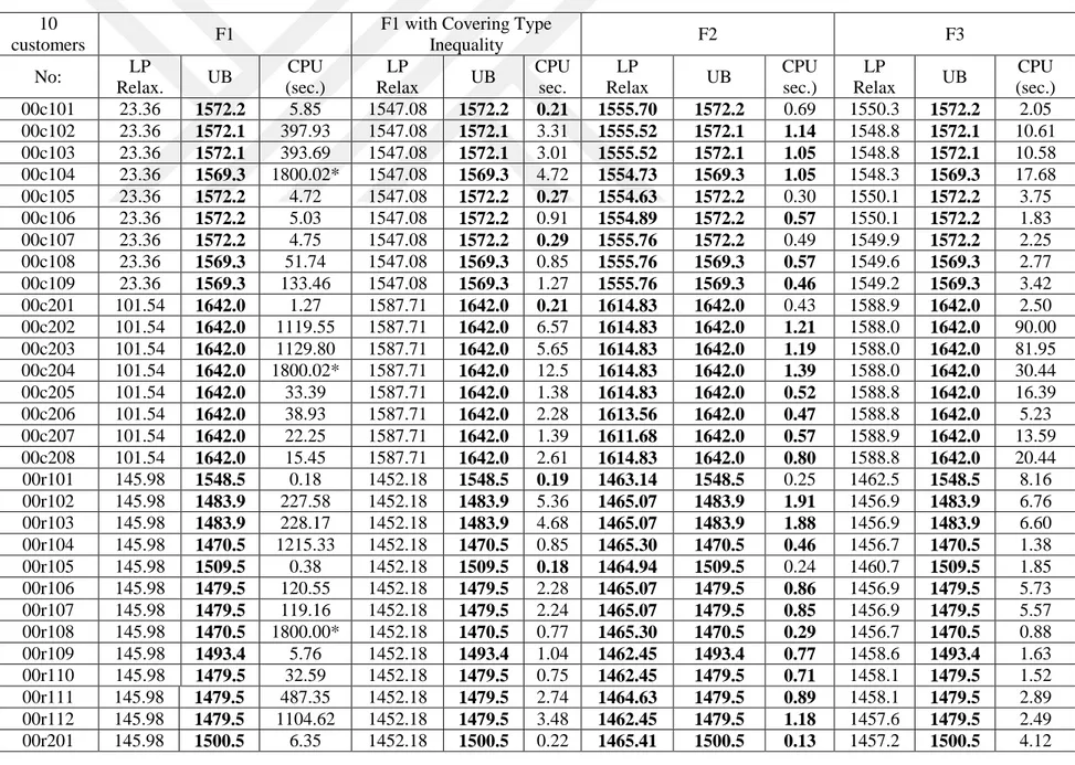
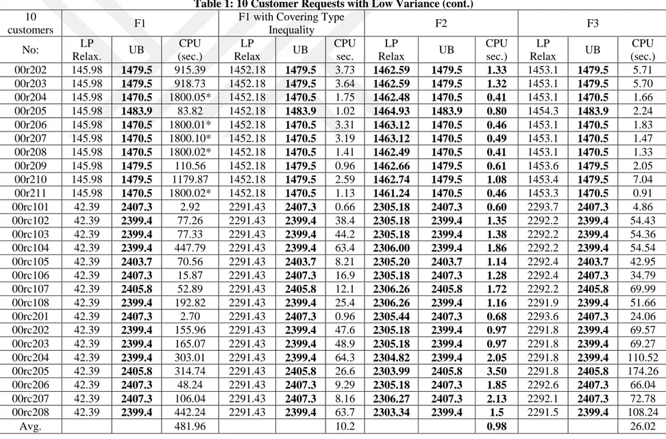
Table 1: 10 Customer Requests with Low Variance ... 35
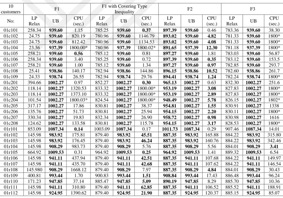
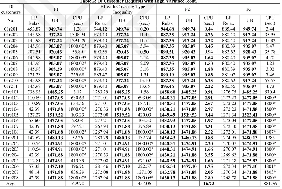
Table 2: 10 Customer Requests with High Variance ... 37
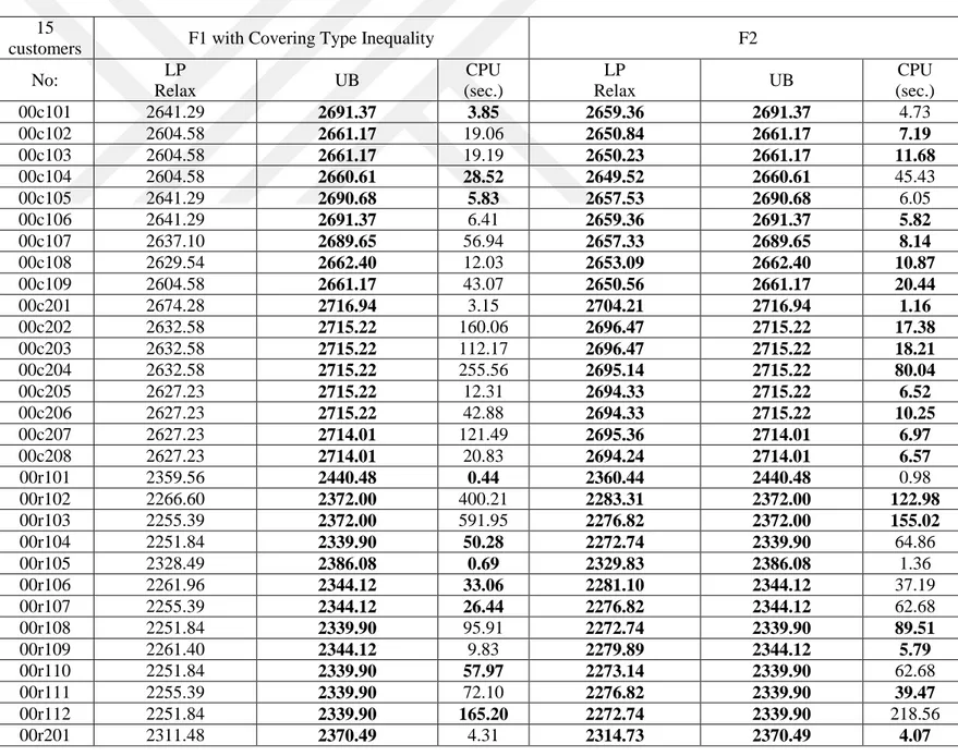
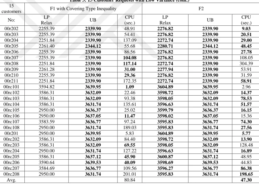
Table 3: 15 Customer Requests with Low Variance ... 40
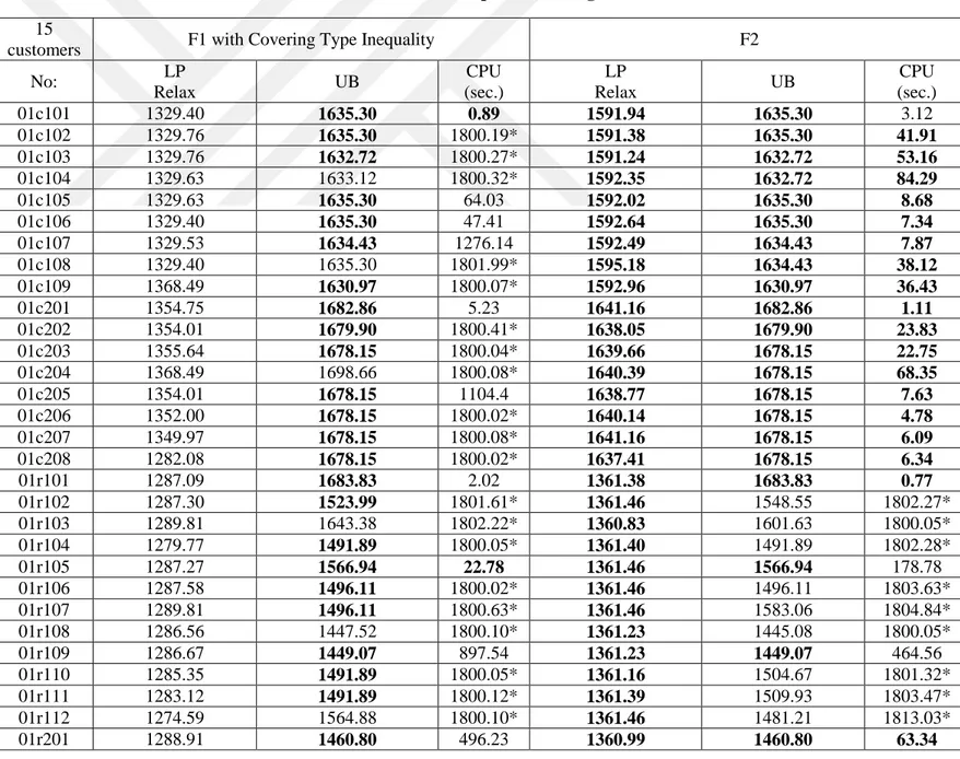
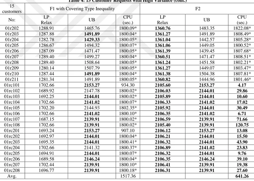
Table 4: 15 Customer Requests with High Variance ... 42
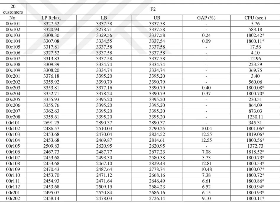
Table 5: 20 Customer Requests with Low Variance ... 44
Table 6: 20 Customer Requests with High Variance ... 46
Table 7: Parameters of ALNS... 48
Table 8: Comparison of F2 and ALNS ... 50
Table 9: Comparison of F2 and ALNS ... 52
Table 10: Results of ALNS on 50 Requests with Low Variance ... 55
Table 11: Results of ALNS on 50 Requests with High Variance ... 56
Table 12: Results of ALNS on 100 Requests with Low Variance ... 58
Table 13: Results of ALNS on 100 Requests with High Variance ... 60
xii
INDEX OF SYMBOLS AND ABBREVIATIONS
Abbreviations Explanations
VRP Vehicle routing problem
CVRP Capacitated vehicle routing problem HVRP Heterogeneous vehicle routing problem VRPTW Vehicle routing problem with time windows
SPDVRP Simultaneous pick-up and delivery vehicle routing problem PDPVRP Pick-up and delivery vehicle routing problem
LP Linear programming
TSP Travelling salesman problem
PDPVRPTW Pick-up and delivery vehicle routing problem with time windows ALNS Adaptive large neighborhood search
LNS Large neighborhood search
HVRPTWSPD Heterogeneous vehicle routing problem with time windows and simultaneous pick-up and delivery
HTW Hard time windows
PD Pick-up and delivery
xiii
ST Single trip
MSTC Minimizing total distance cost
HF Heterogeneous fleet
FC Fixed capacity
SC Single compartment
MCP Multiple compatible product STP Single time period
1
1 INTRODUCTION
One of the main processes in companies is logistics management. It consists of supply of raw materials, transportation of products, stock control etc., among which the most costly process is the transportation of products. Considerable expenses are made for this purpose. Due to this fact, it is obvious that even small improvements in transportation can lead to remarkable overall gains. Therefore, operations research techniques are crucial for the management of logistics operations.
1.1 Subject of the Thesis
The subject of the thesis is developing a problem framework and solution methodologies to a heterogeneous vehicle routing problem with time windows and simultaneous pickup and delivery. The problem handled in this thesis is one of the most comprehensive variants of vehicle routing.
Different variants of the vehicle routing problem were examined and some of the most similar researches were reviewed. Details of the problem such as parameters and constraints were identified. Three different mathematical models were proposed to learn which way of modelling is suitable to the particular problem on hand in terms of obtained lower bounds.
It is known that vehicle routing problem is Hard. Our problem is also NP-Hard, since it generalizes the classical vehicle routing problem. Therefore, to solve real-world instances which are larger than classical benchmark instances, a heuristic approach is also proposed in this thesis. To the best of our knowledge, the problem in this thesis has not been studied in the literature. So, to test proposed mathematical models and proposed heuristic algorithm, a new set of instances was generated. A computational analysis was made, which includes small instances to compare the lower bounds obtained from different formulations, and to compare the results of the proposed heuristic approach to the optimal or best solutions from the developed formulations. Computational analysis also includes larger instances to measure the solution quality of the heuristic, by comparing our heuristic to a simple insertion based heuristic, as there are no available benchmark instances for our problem in the literature.
2
Most of the route planners confront with this problem almost every day. For this reason, a software company wanted us to develop a solution methodology to provide fast and good results for its customers. Therefore, this thesis is motivated from a concrete real life need.
1.2
Aims and Problem DefinitionThe aim of this thesis is to study a problem that has not been studied extensively. The problem has broad application areas from transporting goods to transporting people. The wide application area is critical for us, to be able to provide benefits to practitioners in different sectors, as the study is motivated from a real-life problem. As the total logistics costs are estimated as twenty percent of total production costs in OECD countries (Sudalaimuthu and Raj, 2009), another important aim is to develop an algorithm to obtain good solutions to real world instances, in order to help practitioners in terms of planning time and total logistics costs.
The problem interests any company distributing its products from the depot to some customers. The decisions of which product should be assigned to which vehicle, and determining the routes of the vehicles is of concern. In the problem studied in this thesis, the company may have a heterogeneous fleet where the vehicles may differ from one to another in terms of capacities and costs. We handle the problem from the company’s point of view, considering customer requirements. For example, some customers may request specific time intervals to accept visits from the vehicles, or some customers may have not only delivery demands but also some pickup demands to be transported back to the depot. Therefore, in this study, three extensions of the basic vehicle routing problem are considered: heterogeneous vehicles, time windows and simultaneous pickup and delivery demands.
Therefore, the heterogeneous vehicle routing problem with time windows and simultaneous pick-up and delivery is considered in this thesis, where the objective is to minimize the total fixed cost of the used vehicles and the total travelling cost. To the best of our knowledge, this complex problem has not been studied yet in the vehicle routing literature. Three different types of mathematical models is proposed to formulate the problem. The first one is based on Miller-Tucker-Zemlin (1960) constraints. The other two are based on flow decision variables. A new set of benchmark instances is generated to compare the lower bounds obtained by the
3
mathematical models. The flow variables-based mathematical models give the best results based on computational experiments. As the mathematical models can solve only small sized problem instances to optimality, a heuristic algorithm is also proposed to solve larger real world instances. When the proposed heuristic and the models are compared, the algorithm finds optimal solution in most of the instances, and on the average the algorithm finds better solutions than the mathematical models. For larger instances, we compare the algorithm with a simple insertion heuristic to find that it finds much better solutions than the simple heuristic. The results of the experiments show that the proposed algorithm is not only stable in terms of solution quality but also robust in terms of computational time. As a result, the proposed heuristic algorithm can be securely used in everyday logistics operations to obtain fast and quality results. The proposed algorithm will be embedded in a software package, and will be provided as a logistics planning tool to the customers of the software company.
1.3 Context of the Thesis
The thesis content is based on the routing plan of vehicles in companies, which distribute their products to delivery locations. In the first part, we define the problem framework, which contains parameters and constraints. As the problem is motivated from a real-life need, the vehicle fleet is assumed to be heterogeneous, as most distribution companies have different types of vehicles. Time windows of the customers are respected while minimizing the total transportation cost. The time window of a customer is defined as the time interval in which the customer should receive the delivery by a vehicle. We consider hard time windows, which are identified as strictly determined deadlines. The pickup demands of customers are also included, as these can be seen as returned products, which have a wide application area in reverse logistics.
In the second part of the thesis, we review the literature on similar studies to our problem. Mathematical models of some specific vehicle routing problems are analyzed, and solution approaches are examined. As exact approaches can solve very limited number of instances, we concentrate on heuristic algorithms. In the last part, we propose three different formulations of the problem to examine which way of modeling performs better for obtaining lower bounds. To compare the lower bounds, we propose new sets of instances that consider different types of vehicles, pickup
4
demands and time windows, by extending Solomon’s (1987) benchmark instances. We also propose a heuristic algorithm, inspired from the Adaptive Large Neighborhood Search by Ropke and Pisinger (2006), to solve large practical instances.
1.4 Organization of the Thesis
This thesis consists of six chapters and is organized as follows. The next chapter provides the literature review on related vehicle routing problems in three sections. The first section gives some background information about the vehicle routing problem and its variants. The second section consists of heuristic approaches to solve different variants of the problem. The last section concludes Chapter 2 with a discussion. Chapter 3 provides detailed information about the considered problem; three different mathematical models are presented, and a valid inequality proposed by Yaman (2006) is adapted in this chapter. In Chapter 4, a heuristic algorithm is proposed to obtain approximate solutions to the problem. The algorithm contains several sub-heuristics, and the pseudocode is provided for each. Chapter 5 reports the experimental analysis on the solutions of the mathematical models and the heuristic algorithm on generated test instances. Finally, the conclusions are given and the contributions of the thesis and future directions are discussed in Chapter 6.
5
2 LITERATURE REVIEW
As mentioned in the previous chapter, we consider a single depot, heterogeneous fleet, pick-up and delivery vehicle routing problem with time windows. Early works on vehicle routing problem (VRP) is started with Dantzig and Ramsey (1959). Since that date, VRP has been increasingly getting attention by the operations research community. This chapter is divided into three sections. The next section is a review of different class of VRPs, and the solution approaches are reviewed in the Chapter 2.2.
2.1 Vehicle Routing Problem
The three simpler variants of the problem considered in this study are introduced in this section. These are heterogeneous VRP (HVRP), VRP with time windows (VRPTW), and simultaneous pick-up and delivery VRP (SPDVRP). In the following section, different variants of the VRP are explained and some studies are reviewed. Mathematical definitions are excluded for conciseness. For more detailed information on the problem, we refer the reader to the excellent textbook by Toth and Vigo (2001), and to the survey by Laporte (1992). It should be noted that, since the classical VRP is NP-hard because it generalizes the Travelling Salesman Problem, all three variants are NP-hard, as well.
Heterogeneous Fleet VRP
In the capacitated VRP (CVRP), it is assumed that all vehicles are identical in terms of capacities and costs. The HVRP generalizes the CVRP by considering different types of vehicles. In general, the objective function is minimizing the fixed costs and the routing costs of vehicles. Although it is more realistic and the real-world problems deal with heterogeneous vehicles more than the identical vehicles, the HVRP has received much less attention by the researchers, possibly due to its complexity.
Yaman (2006) also notes that the lack of interest may be caused by the difficulty of finding good lower bounds for HVRP. The reason of the difficulty is that, the fixed costs dominate the routing costs in the optimal solution of the linear
6
programming (LP)-relaxation. Therefore, the vehicles make fractional subtours. Also, Yaman (2006) proposes six different formulations for the HVRP; four of them are based on Miller-Tucker-Zemlin constraints and two are based on flow formulations. Flow formulations lead to much better lower bounds than Miller-Tucker-Zemlin based formulations. However, the computational time of strong formulations increases significantly for large instances. To improve lower bounds, several valid inequalities covering type inequalities, subtour elimination inequalities, generalized large multistar inequalities and valid inequalities based on lifting of the Miller-Tucker-Zemlin constraints are proposed by the author. Computational results show that the valid inequalities, especially covering type inequalities, improve the lower bounds significantly.
The PhD dissertation of Özfırat (2008) considers three different variants of VRP, namely HVRP, split delivery (SDVRP) and VRPTW. A threshold algorithm is proposed to solve HVRP, SDVRP and small-sized VRPTW. The developed threshold algorithm is a two-stage algorithm, where the customers are clustered in the first stage and the routes are determined for each cluster in the second stage. A fuzzy goal programming approach is proposed for the clustering stage, and a constraint programming model is developed for the routing stage. In addition, a set covering algorithm is proposed for large scale VRPTW instances.
Baldacci et al. (2008) reviews different formulations and valid inequalities that are proposed by other researchers. Also, the authors briefly describe heuristic approaches proposed in the literature, and compare computational performances.
VRP with Time Windows
The VRPTW is the extension of the CVRP where each customer has a time interval and a vehicle must visit the customer in that interval. There are two types of time windows, defined as soft and hard. Soft time windows allow the vehicles to visit customers outside their time windows with a penalty cost. On the contrary, the hard time windows cannot be violated. For detailed information, we refer the reader to the surveys by Cordeau et al. (2001), Kallehauge et al. (2005) and Kallehauge (2008). Cordeau et al. (2001) presents a multi-commodity network flow model to formulate VRPTW, and describes different heuristic approaches to derive upper bounds, and
7
two decomposition approaches (Lagrangean relaxation and column generation) for deriving lower bounds. Kallehauge et al. (2005) focuses on column generation approach in general, and path formulation is reviewed extensively. Also, the authors propose several acceleration strategies improving the overall approach considerably. Kallehauge (2008) reviews four types of formulations of Travelling Salesman Problem (TSP), which are the arc formulation, the arc-node formulation, the spanning tree formulation and the path formulation, and gives polyhedral results. The reason for reviewing different formulations of TSP is that, if one applies a decomposition approach, the subproblem can be formulated as TSP. Thus, the TSP forms a basis for the VRPTW. The author also gives a detailed literature review of solution approaches for the path formulation.
It should be noted that the existing solution approaches for the VRPTW are dominated by column generation. One of the most important reasons for this dominance might be the advancements in the solution of the subproblem, which is a path formulation, as there are pseudo-polynomial algorithms for the Shortest Path Problem with Resource Constraints.
Pick-up and Delivery VRP
Another important class of VRP is the pickup and delivery problems (PDVRP). In this problem category, people or goods are to be transported to some destination points. In general, each request is defined by a pickup location and a delivery location. Delivery location may be the same as the pickup location. If that is the case, the problem is called as SPDVRP. Otherwise, the problem has some extra constraints such as coupling and precedence. In the VRP literature, the SPD has not received much attention as other pickup and delivery problems. For more information on PDVRP, we refer the reader to surveys by Berbeglia et al. (2007) and Parragh et al. (2008).
2.2 Heuristic Approaches
In last two decades, several unsolved VRP problem instances have been solved optimally. However, for practical instances, exact algorithms are not reliable for solving the problem in terms of variability of computational time. From a practical point of view, the computational time is as important as the quality of the solution.
8
Therefore, heuristic approaches are still the only viable option for large instances. Several surveys on heuristic approaches have been published. We refer the reader to these surveys by Laporte et al. (2000), Cordeau et al. (2005), and Vidal et al. (2013) for detailed information.
Dethloff (2001) proposes a simple insertion-based heuristic for simultaneous pick-up and delivery VRP. The insertion heuristic includes the function of the total length of vehicle, the function of the remaining capacity of vehicle, and a distance function which prevents the late and unfavorable insertions of distant located customers. The algorithm starts with selecting a seed customer to create a route. The insertion cost is calculated for all unassigned customers (the customers who has not assigned to any vehicle/route) for each possible insertion to the route. Then the best candidate in terms of minimum cost is assigned to the route. This step is continued until no unassigned customer can be inserted into the route. After that step, if there are some unassigned customers, a new route is created with the same steps. The computational complexity of this very fast algorithm is 𝑂(𝑛4). However, the algorithm assumes homogenous vehicles and does not consider the time window constraints.
Li and Lim (2003) use a metaheuristic approach to solve the pick-up and delivery VRP with time windows (PDPVRPTW). The proposed algorithm is a hybrid method of simulated annealing and tabu search. The algorithm starts with finding an initial solution by using a simple insertion method. Then to find better feasible solutions, three types of neighborhood structures are used within a simulated-annealing-like multiple-restart strategy. The algorithm also contains a tabu list to avoid cycling.
Lu and Dessouky (2006) develop an insertion-based heuristic for solving the PDVRPTW. The insertion heuristic considers the total length of the route as well as the total slack time of the time windows. In addition, a nonstandard measure “crossing length percentage” is presented to determine the visual attractiveness of the solution. Its value takes zero if the route does not have any crossing points in itself, and the value increases with respect to the length of the crossing distance. The routes with high crossing length percentage values are not accepted. The algorithm can be summarized as follows: Initial routes are determined by solving a maximum clique problem with a greedy algorithm. The solution gives a set of customers which cannot
9
be assigned to the same route. Then the insertion cost is calculated for each unassigned customer for each possible insertion to the routes. This process is continued until there is no customer to be assigned. The computational complexity of the algorithm is 𝑂(𝑛4). However, this algorithm also assumes the vehicles are identical.
Ropke and Pisinger (2006), and Pisinger and Ropke (2007) mention that there are many heuristic methods in the literature, but these methods have highly strict structures for specific VRP variants. These restrictions prevent the algorithms from applying to different problem types. Thus, the authors propose an algorithm that can be applied to five different VRP variants: VRPTW, CVRP, multi depot VRP, open VRP, and site-dependent VRP. First, the problems are transformed into PDVTPTW. Then, Adaptive Large Neighborhood Search (ALNS) is employed, which is an extension of the large scale neighborhood search heuristic of Shaw (1997, 1998). ALNS includes several insertion and removal heuristics, and applies these heuristics with an adaptive layer. In each iteration, a removal heuristic is selected to remove a predetermined number of customer requests from routes, and an insertion heuristic is selected to insert the unassigned customer requests to the routes. The selection of heuristics is adaptively made by considering the contribution in previous iterations. More information on Large Neighborhood Search (LNS) can be found in a survey proposed by Pisinger and Ropke (2010). The computational results show that the proposed algorithm is very stable in terms of the solution quality. The only disadvantage of the algorithm is, as ALNS is a metaheuristic, there are several parameters to fine-tuned. Due to the effectiveness of ALNS, the number of papers employing ALNS has been increasing in recent years (Riberio and Laporte, (2012), Hemmelmayr et al., (2012), Demir et al., (2012), Azi et al., (2014) Luo et al., 2016)).
2.3 Discussion
Vehicle routing has been getting attention from the operations researchers for a long time. This interest leads researchers to study different variants of the problem. Also, as the different variants have been studied, a lot of effective algorithms have been proposed. However, the mainstream of the research focused on solving some benchmark problem instances better than others. In our opinion, it will be better to study practical realistic variants of the problem by a utilitarian approach. In other words, studying variants of the problem that have not received much attention despite
10
their broad application areas might be worthwhile from a practical point of view. For this purpose, we study the heterogeneous vehicle routing problem with time windows and simultaneous pickup and delivery (HVRPTWSPD). To the best of our knowledge, this problem has not been studied in the literature.
A recent study (Taşar, 2016) proposes a taxonomy for the VRP, which involves a five-field notation including operational policy, objective function, vehicle features, product features and the planning period. While operational policy field includes time windows, carrying types, split deliveries and trips, the objective function field contains minisum, minimax and load balancing type objectives. Vehicle features involve fleet type, capacity and compartment and the product features represent different product types in the problem. Finally, the planning period field contains the number of periods. Based on this notation, our operational policies include hard time windows (HTW), pick-up and delivery (PD), no split delivery (SP’) and single trip (ST). Our objective function is minimizing the total distribution cost (MSTC). The vehicle features are heterogeneous fleet (HF), fixed capacity (FC) and single compartment (SC), while the product features include multiple compatible products (MCP). Our planning period is a single time period (STP). Hence, our problem can be represented as follows, using the taxonomy by Tasar (2016):
HTW, PD, SP’, ST | MSTC | HF, FC, SC | MCP | STP.
In the next chapter, we examine the details of the problem and propose three different formulations.
11
3 PROBLEM FRAMEWORK AND MATHEMATICAL FORMULATIONS
In this study, three extensions of the basic vehicle routing problem are considered together, which are VRPTW, HVRP and SPDVRP. It should be noted that this practical problem has been brought to our attention by a software company, which needed to form a route optimization algorithm as a logistics planning tool for its customers.
At the beginning of a planning day, all vehicles are ready to start their routes at the depot. When a vehicle is loaded with a set of customer delivery demands, it starts its route at time 0. Next, the vehicle visits its first customer to satisfy their delivery demand. If the customer has a pick-up demand as well, the pick-up demand must be picked up by the same vehicle at the same time. Hence, we assume that each customer is visited exactly once. For representation purposes, it is assumed that depot has zero pick-up and delivery demand. The arrival time of the vehicle to the first customer is the departure time from the depot plus the travel time between the depot and the first customer. If there is any service time at the depot, that must also be included in the arrival time to the first customer. The vehicle visits all its assigned customers in its route in the same manner, before returning to the depot. The vehicles may differ from each other in terms of their capacities, fixed costs, and cost per kilometer. We assume that the customers and the depot have time windows for receiving their service by a vehicle, i.e. a vehicle arriving to a customer before the start of their time window should wait until the start. Similarly, it is not allowed to serve a customer after the end of the customer’s time window. Latest arrival time to the depot indicates the permissible working hours of the vehicles. The objective function is to minimize the total fixed cost of vehicles, as well as total travelling costs.
The problem can be formulated as follows: 𝐺 = (𝑉, 𝐴) is a complete directed graph with node set 𝑉 = {0, 1, … , 𝑛, 𝑛 + 1} and arc set 𝐴 = {(𝑖, 𝑗): 𝑖, 𝑗 ∈ 𝑉, 𝑖 ≠ 𝑗}. Nodes 0 and 𝑛 + 1 denote the initial and the terminal depot, which may correspond to the same geographical location. Subset 𝑉𝑐 = {1,2, … , 𝑛} denotes customer nodes. All vehicles start their routes at node 0 and finish at node 𝑛 + 1. The set 𝐾 = {1, … , 𝑚} denotes the vehicles, while 𝑚 represents the number of available vehicles.
12
In this thesis, we propose three different formulations to the problem. The first formulation is based on Miller-Tucker-Zemlin (1960) constraints, and the last two are based on flow variables. The following parameters and decision variables are common to the three formulations.
Common Parameters:
𝑑𝑖: delivery demand of node 𝑖 ∈ 𝑉. 𝑝𝑖: pick-up demand of node 𝑖 ∈ 𝑉.
𝑡𝑖,𝑗: distance between node 𝑖 and node 𝑗, (𝑖, 𝑗) ∈ 𝐴. ℎ𝑖: service time of node 𝑖 ∈ 𝑉.
[𝑎𝑖, 𝑏𝑖]: earliest and latest possible arrival time of node 𝑖 ∈ 𝑉. 𝑐𝑘: capacity of vehicle 𝑘 ∈ 𝐾.
𝛾𝑘: fixed cost of vehicle 𝑘 ∈ 𝐾.
𝛼𝑘: cost per kilometer of vehicle 𝑘 ∈ 𝐾. 𝛽𝑘: average speed of vehicle 𝑘 ∈ 𝐾.
𝑀: A large number, e.g. 𝑀 = max {∑𝑖∈𝑉𝑑𝑖+ 𝑝𝑖, ∑(𝑖,𝑗)∈𝐴𝑡𝑖,𝑗}.
Common Decision Variables:
𝑥𝑖,𝑗𝑘 : 1, if vehicle 𝑘 ∈ 𝐾 travels directly from node 𝑖 ∈ 𝑉 to node 𝑗 ∈ 𝑉. 0, otherwise. 𝑤𝑘: 1, if vehicle 𝑘 ∈ 𝐾 is used. 0, otherwise.
3.1 Formulation 1: Basic Formulation
13 Additional Decision Variables:
𝑠𝑖𝑘: the time vehicle 𝑘 ∈ 𝐾 arrives at node 𝑖 ∈ 𝑉. 𝑙𝑖𝑘: the load of vehicle 𝑘 ∈ 𝐾 after leaving node 𝑖 ∈ 𝑉.
With the above definitions, the mathematical model becomes:
min: ∑(𝑖,𝑗)∈𝐴∑𝑘∈𝐾𝛼𝑘𝑡𝑖,𝑗𝑥𝑖,𝑗𝑘 + ∑𝑘∈𝐾𝛾𝑘𝑤𝑘 (0) subject to: ∑𝑖∈𝑉∑𝑘∈𝐾𝑥𝑖,𝑗𝑘 = 1 𝑗 ∈ 𝑉𝑐 (1) ∑𝑖∈𝑉𝑥𝑖,𝑗𝑘 − ∑𝑖∈𝑉𝑥𝑗,𝑖𝑘 = 0 𝑗 ∈ 𝑉𝑐, 𝑘 ∈ 𝐾 (2) 𝑠𝑗𝑘 ≥ 𝑠𝑖𝑘+𝑡𝑖,𝑗 𝛽𝑘 ⁄ + ℎ𝑖− 𝑀(1 − 𝑥𝑖,𝑗𝑘) (𝑖, 𝑗) ∈ 𝐴, 𝑘 ∈ 𝐾 (3) 𝑎𝑖 ≤ 𝑠𝑖𝑘 ≤ 𝑏𝑖 𝑖 ∈ 𝑉, 𝑘 ∈ 𝐾 (4) 𝑙𝑗𝑘 ≥ 𝑙𝑖𝑘+ 𝑝𝑖 − 𝑑𝑖− 𝑀(1 − 𝑥𝑖,𝑗𝑘 ) (𝑖, 𝑗) ∈ 𝐴, 𝑘 ∈ 𝐾 (5) 𝑙0𝑘 = ∑(𝑖,𝑗)∈𝐴𝑑𝑖𝑥𝑖,𝑗𝑘 𝑘 ∈ 𝐾 (6) 𝑙𝑖𝑘 ≤ 𝑐𝑘 𝑖 ∈ 𝑉, 𝑘 ∈ 𝐾 (7) ∑𝑗∈𝑉𝑐𝑥0,𝑗𝑘 = 𝑤 𝑘 𝑘 ∈ 𝐾 (8) 𝑥𝑖,𝑗𝑘 ∈ {0, 1} (𝑖, 𝑗) ∈ 𝐴 , 𝑘 ∈ 𝐾 (9) 𝑠𝑖𝑘, 𝑙𝑖𝑘∈ ℝ+ 𝑖 ∈ 𝑉, 𝑘 ∈ 𝐾 (10)
14
The objective function minimizes the fixed cost of vehicles and the total travel cost. Constraint set (1) ensures that each customer request is satisfied. Constraint set (2) guarantees that, if a vehicle visits one node it must leave that node. Constraint set (3) imposes consistency of the visiting times of nodes. Constraint set (4) ensures that the arrival times of nodes are within time windows. Constraint set (5) imposes consistency of loads of vehicles. Constraint set (6) determines the load of vehicles upon leaving the depot. Constraint set (7) ensures that the vehicle capacities are not exceeded. Constraint set (8) determines which vehicles are used. Constraint sets (9) and (10) represent the ranges of decision variables.
3.2 Formulation 2: Demand Flow Formulation
The second formulation is based on demand flow variables. Two additional decision variables are used to represent pick-up and delivery demand quantities along arcs.
Additional Decision Variables:
𝑠𝑖𝑘: the time which vehicle 𝑘 ∈ 𝐾 arrives at node 𝑖 ∈ 𝑉. 𝑓𝑖,𝑗+: the delivery demand flow of arc (𝑖, 𝑗) ∈ 𝐴.
𝑓𝑖,𝑗−: the pick-up demand flow of arc (𝑖, 𝑗) ∈ 𝐴.
With the additional decision variables, the mathematical model becomes: min: (0)
subject to:
(1) − (4), (8) − (9), and
15 ∑𝑘∈𝐾𝑑𝑗𝑥𝑖,𝑗𝑘 ≤ 𝑓𝑖,𝑗+ ≤ ∑𝑘∈𝐾(𝑐𝑘− 𝑑𝑖)𝑥𝑖,𝑗𝑘 (𝑖, 𝑗) ∈ 𝐴 (12) ∑𝑗∈𝑉𝑓𝑖,𝑗− − ∑𝑗∈𝑉𝑓𝑗,𝑖− = 𝑝𝑖 𝑖 ∈ 𝑉𝑐 (13) ∑𝑘∈𝐾𝑝𝑖𝑥𝑖,𝑗𝑘 ≤ 𝑓𝑖,𝑗− ≤ ∑𝑘∈𝐾(𝑐𝑘− 𝑝𝑗)𝑥𝑖,𝑗𝑘 (𝑖, 𝑗) ∈ 𝐴 (14) 𝑓𝑖,𝑗++ 𝑓𝑖,𝑗− ≤ ∑𝑘∈𝐾𝑐𝑘𝑗𝑥𝑖,𝑗𝑘 𝑘 ∈ 𝐾 (15) 𝑠𝑖𝑘, 𝑓𝑖,𝑗+, 𝑓𝑖,𝑗− ∈ ℝ+ (𝑖, 𝑗) ∈ 𝐴, 𝑘 ∈ 𝐾 (16)
Constraint set (11) guarantees that the amount of delivery flow 𝑑𝑗 should be sent to node 𝑗 ∈ 𝑉𝑐. Constraint set (12) ensures that, if arc (𝑖, 𝑗) ∈ 𝐴 is traversed by a vehicle, delivery flow on it should be at least the delivery demand of node 𝑗 ∈ 𝑉𝑐, and the delivery flow on the arc cannot exceed the capacity of the vehicle. Constraint set (13) guarantees that, amount of pick-up flow 𝑝𝑖 should be sent to node 𝑖 ∈ 𝑉𝑐. Constraint set (14) ensures that if arc (𝑖, 𝑗) ∈ 𝐴 is traversed by a vehicle, the delivery flow on it should be at least the pick-up demand of node 𝑖 ∈ 𝑉𝑐, and the delivery flow on the arc cannot exceed the capacity of the vehicle. Constraint set (15) ensures that vehicle capacity is not exceeded. Constraint set (16) represents the range of decision variables.
3.3 Formulation 3: Time Flow Formulation
The third formulation is based on time flow variables. An additional decision variable is used to represent time flow along arcs.
Additional Decision Variables:
𝑙𝑖𝑘: the load of vehicle 𝑘 ∈ 𝐾 after leaving node 𝑖 ∈ 𝑉.
16
With the above additional decision variables, the mathematical model becomes: min: (0) subject to: (1) − (2), (5) − (9), and ∑𝑗∈𝑉𝑠𝑖,𝑗 ≥ ∑𝑗∈𝑉𝑠𝑗,𝑖+ ∑𝑗∈𝑉∑𝑘∈𝐾𝑥𝑗,𝑖𝑘(𝑡𝑗,𝑖 𝛽𝑘 ⁄ + ℎ𝑖) 𝑖 ∈ 𝑉 (17) ∑𝑘∈𝐾𝑥𝑖,𝑗𝑘 (𝑎𝑖− ℎ𝑖) ≤ 𝑠𝑖,𝑗 ≤ ∑𝑘∈𝐾𝑥𝑖,𝑗𝑘 (𝑏𝑖 − ℎ𝑖) 𝑖 ∈ 𝑉 (18) 𝑠𝑖,𝑗, 𝑙𝑖𝑘 ∈ ℝ+ (𝑖, 𝑗) ∈ 𝐴, 𝑘 ∈ 𝐾 (19)
Constraint set (17) determines the time a vehicle leaves node 𝑖 ∈ 𝑉. Constraint set (18) ensures that the arrival time to the nodes must be within their respective time windows. Constraint set (19) represents the range of decision variables.
3.4 Valid Inequality
As mentioned in the literature review, the LP-relaxation solution of the HVRP is too weak (Yaman, 2006). The other disadvantage of solving the HVRP is, since the capacities and costs of the vehicles are different, the selection of which vehicles are used is crucial. This situation significantly increases the size of branch-and-bound tree in the exact solution. Therefore, the compound effect of these two difficulties makes the problem hardly solvable even for small instances. This fact is verified in our computational experiments, as well. To overcome these disadvantages, Yaman (2006) proposed several valid inequalities to the HVRP. The most promising valid inequality is the covering type inequality, which is also valid for the HVRP with time windows. Therefore, we add this inequality to our formulations for Q>0, as follows: ∑ ∑ ⌈𝑐𝑘⁄ ⌉ 𝑥𝑄 0,𝑗𝑘 ≥ ∑ ⌈𝑑𝑖 𝑄 ⁄ ⌉ 𝑖∈𝑉𝑐 𝑘∈𝐾 𝑗∈𝑉𝑐 (20)
17
4 SOLUTION APPROACH
As the VRP is NP-Hard, it is quite difficult to solve real-world instances. Under heterogeneous vehicles assumption, it is harder to solve even small instances optimally. In this thesis, a heuristic approach is proposed to overcome this difficulty. Our heuristic is inspired by the algorithm of Ropke and Pisinger (2006), namely the Adaptive Large Neighborhood Search (ALNS), which was developed for the PDVRPTW. In our case the problem is HVRPTWSPD, which leads to two extensions in the algorithm; computing the necessary number of vehicles, and a new insertion heuristic for time windows. The proposed heuristic consists of two stages. The main objective is minimizing the number of vehicles, and the second aim is minimizing the total travelling distance of the vehicles. The algorithm considers all assumptions of the problem like time windows, pickup demands, and heterogeneous fleet.
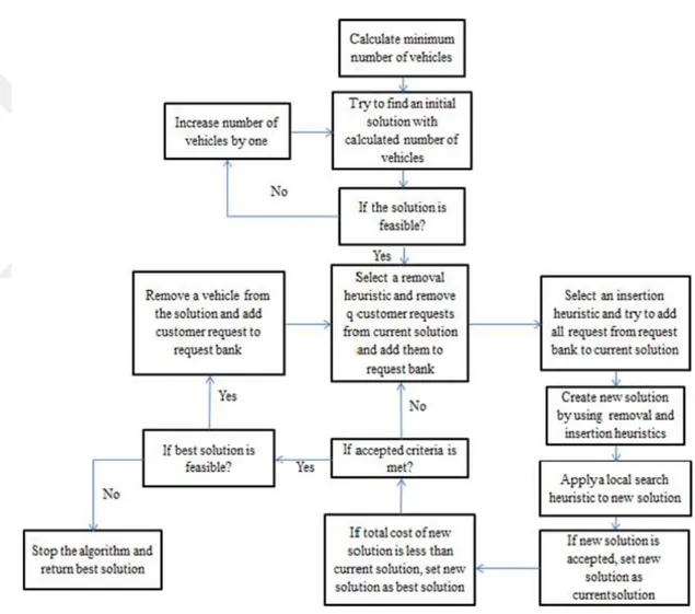
The details of the proposed heuristic are explained in the following sections. Also, a flow chart is presented in Figure 1. The underlined words below indicate the heuristics (subroutines) explained in this chapter.
The ALNS Heuristic:
S1. Calculate the Minimum Number of Vehicles.
S2. Find an Initial Solution. Set this solution as the current solution and the incumbent solution.
S3. If the solution is infeasible, increase the number of vehicles and go to S2. Otherwise, go to S4.
S4. Generate new solution:
a. Select a Removal heuristic based on removal heuristic scores, and apply to the current solution.
b. Select an Insertion Heuristic based on insertion heuristic scores, and apply to the current solution.
S5. Apply a Local Search algorithm to the new solution.
S6. If the Acceptance Criteria is met, set new solution to the current solution. S7. Update Heuristic Scores.
18 current solution to the best solution.
S9. If the Stopping Criteria is met, go to S10. Otherwise, go to S4.
S10. If the last found incumbent solution is feasible, decrease the number of vehicles by one and go to S2. Otherwise, go to S11.
S11. Report the last found best solution.
Figure 1: Flow Chart of the Heuristic.
4.1 Minimum Number of Vehicles Heuristic
The heuristic algorithm starts with finding a lower bound on the needed number of vehicles. Unlike our strategy, Ropke and Pisinger (2006) starts by finding an upper
19
bound on the number of vehicles. The advantage of starting with a lower bound instead of an upper bound is decreasing the total computation time of the algorithm. As the initial solution algorithm is regret-2, it finds a solution very quickly, as it will be explained later. This way, the main part of the heuristic can spend more time to improve the initial solution with the least number of vehicles.
Finding a minimum number of vehicles becomes a variant of the bin packing problem. As the vehicle fleet is heterogeneous, the bins are heterogeneous as well. However, it is time consuming to solve this problem to optimality as the bin packing problem is NP-Hard. Also, in our problem, the lower bound on the number of vehicles may be weak due to the existence of the time windows. Therefore, bin packing with heterogeneous bins problem is solved by an adaptation of the Best-Fit Decreasing heuristic (A-BFD), proposed by Crainic et al. (2011). The pseudocode of the algorithm is below.
Inputs:
𝑉𝑐: Set of customers 𝐾: Set of vehicles
𝑆: Set of selected vehicles (S = {∅}) 𝑑𝑖: Delivery demand of customer 𝑖 ∈ 𝑉𝑐 𝑝𝑖: Pickup demand of customer 𝑖 ∈ 𝑉𝑐 𝑣𝑖: 𝑣𝑖 = max{𝑑𝑖, 𝑝𝑖}, 𝑖 ∈ 𝑉𝑐
𝛾𝑘: Fixed cost of vehicle 𝑘 ∈ 𝐾 𝑐𝑘: Capacity of vehicle 𝑘 ∈ 𝐾
20
Sort the vehicles in 𝐾 in their nonincreasing order of ratio 𝛾𝑘 𝑐𝑘
⁄ , 𝑘 ∈ 𝐾 , and nondecreasing order of ck when the fixed costs γk, k ∈ K are equal.
Minimum Number of Vehicles (Crainic et al., 2011) FOR All customer requests 𝑖 ∈ 𝑉;
IF Customer request 𝑖 can be assigned to a vehicle in 𝑆
Assign the customer request 𝑖 to the best vehicle in 𝑆 (vehicle with maximum idle capacity)
ELSE
Add the first vehicle, 𝑏′, in 𝐾 to the 𝑆, 𝑆 = 𝑆 ∪ {𝑏′}, and assign the customer request 𝑖 to vehicle 𝑏′
ENDIF ENDFOR
FOR All vehicles, 𝑗 ∈ 𝑆;
FOR All vehicles, 𝑘 ∈ 𝐾\𝑆; 𝑈𝑗 = ∑𝑖 𝑙𝑜𝑎𝑑𝑒𝑑 𝑖𝑛 𝑗𝑣𝑖 IF 𝑐𝑘 ≥ 𝑈𝑗 and, 𝛾𝑘 < 𝛾𝑗
Move all customer requests from 𝑗 to 𝑘 ENDIF
ENDFOR ENDFOR
Return the vehicles in 𝑆 and the total number of vehicles, (|𝑆|)
4.2 Initial Solution
As stated in the previous section, the initial solution is found by regret-2 heuristic, which is explained in the insertion heuristic section. At the beginning of the algorithm, all customer requests are placed into a request bank, and regret-2 is run in parallel for all vehicles found by the Minimum Number of Vehicles heuristic. If the initial solution is infeasible, the first unused vehicle in 𝐾 is added to the selected vehicles set 𝑆. This procedure is repeated until a feasible solution is found.
21
4.3 Removal Heuristics
The removal heuristics remove a predetermined number of customer requests from the current solution, and add them to the request bank. The request bank contains a set of customer requests not assigned to any vehicle. We propose three types of removal heuristics, as random, worst, and Shaw Removal.
Random Removal
This is a simple removal heuristic that selects r customer requests at random, and removes them from the current solution, as can be seen in the pseudocode below. The idea of random removal is applying randomization to the search process.
Inputs:
𝑛: Total number of customer requests
𝑟: Total number of removed customer requests 𝑋: 𝑆et of customer requests in the current solution 𝐷: Request bank
Random Removal
WHILE 𝑟 customer request is selected;
Select a customer requests at random from 𝑋 and remove the selected demand from the current solution, and assign it into the request bank, 𝐷
ENDWHILE
Return the request bank and new solution
Worst Removal
This subroutine selects r customer requests from the current solution that are most costly, and removes them from the solution. To achieve this, the costs of all customer requests are determined by removing the demand from the solution and
22
calculating cost of the demand. As the demands placed in the request bank have high cost, they are not assigned to the request bank but removed temporarily from the solution. Then, the customer request with the highest cost is removed. The details of the worst removal heuristic are provided in the following pseudocode.
Inputs:
𝑥: Current solution 𝐷: Request bank
𝑓(𝑥): Cost of the current solution
𝑓−𝑖: Cost of current solution after customer request 𝑖 is removed ∆𝑓𝑖: Cost of customer request 𝑖
∆𝑓𝑖 = 𝑓(𝑥) − 𝑓−𝑖 (21)
Worst Removal
WHILE 𝑟 customer request is selected;
FOR All customer requests in solution, 𝑖 ∈ 𝑥; Calculate the cost (21) of customer 𝑖 ENDFOR
Select the customer with the highest cost and remove it from the solution 𝑥, and add to the request bank, 𝐷
ENDWHILE
Return the request bank and new solution
Shaw Removal
This heuristic was proposed by Shaw (1997, 1998). The aim is removing customer requests from the current solution that are similar in terms of their delivery and pickup demands and locations. The idea is to reassign such requests to the same
23
vehicle, if possible. The heuristic starts by selecting and removing a customer request at random from the current solution, and assigning this customer to the removed list. Then, it randomly selects a customer request from the removed list and calculates the similarity of the selected customer and the rest of the customers by using a relatedness measure. The most similar customer request is removed from the solution, and added to the removed list. These steps are repeated until r customer requests are removed from the current solution. The pseudocode of the heuristic is below.
Inputs:
𝑉𝑐: Set of customers 𝐵: Removed list 𝐷: Request bank 𝑥: Current solution
𝑡𝑖,𝑗: Distance between customer 𝑖 ∈ 𝑉𝑐 and customer 𝑗 ∈ 𝑉𝑐
𝑑𝑖: Delivery demand of customer 𝑖 ∈ 𝑉𝑐 𝑝𝑖: Pickup demand of customer 𝑖 ∈ 𝑉𝑐
𝑅𝑖,𝑗: Relatedness measure of customer 𝑖 and 𝑗
𝑅𝑖,𝑗= 𝛼 ∗ 𝑡𝑖,𝑗+ 𝛽 ∗ (|𝑑𝑖 − 𝑑𝑗| + |𝑝𝑖− 𝑝𝑗|) (22) Shaw Removal (Shaw, 1997)
Remove a customer request from solution 𝑖 ∈ 𝑥 at random, and assign it to the removed list, 𝐵.
Select a customer at random from removed list, 𝑖 ∈ 𝐵 WHILE 𝑟 − 1 customer request is removed;
24 Calculate 𝑅𝑖,𝑗 (22)
ENDFOR
Remove the customer from the solution with the lowest 𝑅𝑖,𝑗 value, and assign it to removed list 𝑗 ∈ 𝐵
ENDWHILE
Move all customer requests from 𝐵 to 𝐷 and return new solution
4.4 Insertion Heuristics
There are two main types of insertion heuristics in the VRP literature, which are sequential insertion and parallel insertion. Sequential insertion methods construct routes one by one whereas parallel insertion constructs several routes concurrently. Our proposed algorithm contains three parallel insertion heuristics, as Greedy, Regret, and Time Windows Insertion.
Greedy Insertion
In this basic insertion heuristic, all customer requests from the request bank are tried for all possible positions in vehicles, to calculate an insertion cost for each position. If a request cannot be inserted to a position, the cost is set to infinity. Then, the customer request with the least insertion cost is assigned to its determined position and vehicle. These steps are repeated until the request bank is empty or no insertion is possible. Since only one route is changed at each iteration, the insertion costs for the other vehicles do not need to be calculated. This implementation improves the computation time of all insertion heuristics. The pseudocode is below. Inputs:
𝐷: Request bank
𝑆: Set of vehicles used in new solution
25
∆𝑖,𝑘,𝑗𝑙 : change in objective value by inserting customer 𝑘 between customers 𝑖 and 𝑗 in route l
∆𝑖,𝑘,𝑗𝑙 = 𝑡𝑖,𝑘+ 𝑡𝑘,𝑗− 𝑡𝑖,𝑗 (23)
Greedy Insertion
WHILE All customer requests from request bank, 𝐷, are assigned or no more requests can be assigned;
FOR All customer requests from request bank, 𝑖 ∈ 𝐷; FOR All vehicles, 𝑘 ∈ 𝑆;
Calculate (23) for 𝑖 ∈ 𝐷 and for each position in 𝑘 ∈ 𝑆 ENDFOR
ENDFOR
Assign customer request which have least insertion cost to determined position and vehicle, and remove the request from request bank
ENDWHILE
Update and return the new solution
Regret Insertion
Regret heuristics have been used by Potvin and Rousseau (1993). These insertion heuristics try to improve the basic greedy approach through not only using the best position, but also the second and the third best positions (depending on choice). Customer requests are assigned to positions in order to maximize the regret or opportunity cost, computed as the difference between the best and the second (or the third) best position costs. In this respect, the greedy heuristic can be seen as regret-1 heuristic. In our algorithm, we use regret-2 and regret-3 insertions.
Inputs:
𝐷: Request bank
26
𝑡𝑖,𝑗: Distance between customer 𝑖 ∈ 𝑉𝑐 and customer 𝑗 ∈ 𝑉𝑐
∆𝑖,𝑘,𝑗𝑙 : Change in objective value by inserting customer 𝑘 between customers 𝑖 and 𝑗 in route l
𝑐𝑜𝑠𝑡𝑘𝑞: Minimum 𝑞th cost of customer request 𝑘 , i. e. , 𝑐𝑜𝑠𝑡𝑘1 = min 𝑖,𝑗,𝑙{∆𝑖,𝑘,𝑗
𝑙 }
Regret-m Insertion
WHILE All customer requests are assigned or no more requests can be assigned FOR All customer requests from request bank, 𝑖 ∈ 𝐷;
FOR All vehicles, 𝑘 ∈ 𝑆;
Calculate (23) for customer request 𝑖 and all feasible positions in vehicle 𝑘
ENDFOR ENDFOR
Assign customer request which have maximum regret-m value, ∑𝑚𝑙=2 𝑐𝑜𝑠𝑡𝑖𝑚 − 𝑐𝑜𝑠𝑡𝑖1, 𝑖 ∈ 𝐷 to the determined position and vehicle. Remove the assigned request from request bank
ENDWHILE
Update and return the new solution
Time Windows Insertion
Time windows insertion (Lu and Dessouky, 2006) is different from the regret heuristics in the sense that it considers the time windows of the customers and the waiting times of the vehicles as a cost function instead of the distances between customers. The cost function contains the difference between the time window end time of a customer and the arrival time to that customer, which is named as slack in
the time window; and the time window start time of a customer and the arrival time to
that customer, which is called the waiting time. We use a simple algorithm to evaluate the cost function. The pseudocode of our time insertion heuristic is shown below.
27 Inputs:
Let following be a route that starts from depot and visits 𝑘 customers: 0, 𝑣1, … , 𝑣𝑖−1, 𝑣𝑖, 𝑣𝑖+1, … , 𝑣𝑘, 𝑛 + 1;
𝐷: Request bank
𝑆: Set of vehicles used in new solution
𝑎𝑖: Earliest possible arrival time of node 𝑖 ∈ 𝑉 𝑏𝑖: Latest possible arrival time of node 𝑖 ∈ 𝑉 ℎ𝑖: Service time of node 𝑖 ∈ 𝑉
𝑡𝑖,𝑗: Distance between node 𝑖 ∈ 𝑉 and node 𝑗 ∈ 𝑉 𝐴𝑖: Earliest arrival time of node 𝑖 ∈ 𝑉
𝐴𝑣𝑖 = max(𝐴𝑣𝑖−1, 𝑏𝑣𝑖−1) + ℎ𝑣𝑖−1+ 𝑡𝑣𝑖−1,𝑣𝑖 (24)
𝑊𝑖: Waiting time at node 𝑖 ∈ 𝑉
𝑊𝑣𝑖 = max(0, 𝑎𝑣𝑖−1 − 𝐴𝑣𝑖−1) (25)
𝑌𝑖: Maximal postponed time interval of node 𝑖 ∈ 𝑉
𝑌𝑣𝑖 = { 𝑏𝑣𝑘− max(𝑎𝑣𝑘, 𝐴𝑣𝑘), 𝑖 = 𝑘
min{𝑏𝑣𝑖− max(𝑎𝑣𝑘, 𝐴𝑣𝑘), 𝑌𝑣𝑖+1 + 𝑊𝑣𝑖+1} , 𝑖 = 𝑘 − 1, … ,1 (26)
Time Windows Insertion
28
FOR All customer requests from request bank, 𝑖 ∈ 𝐷; FOR All vehicles, 𝑘 ∈ 𝑆;
Calculate (24), (25) and (26) for customer request 𝑖 ∈ 𝐷 and for all feasible locations in 𝑘 ∈ 𝑆
ENDFOR ENDFOR
Assign customer request which have the largest value of summation of (25) and (26) to determined position and vehicle
ENDWHILE
Update and return the new solution
4.5 Local Search Heuristics
After applying removal and insertion heuristics, we keep this solution as the new solution. Then, a local search heuristic is applied to the new solution for improvement. One of two types of local search heuristics is employed, at random.
Swap-Based Local Search Heuristic
Swap-based local search heuristic chooses two customer requests at random and interchanges them. If the new solution is feasible and costs less, the heuristic is re-called. The process is repeated until the new solution is infeasible or its cost larger. Inputs:
𝑥′: New solution
29 Swap Heuristic
DO
Select a customer request at random from the new solution, 𝑖 ∈ 𝑥′.
Select another customer request at random from the new solution, 𝑗 ∈ 𝑥′\{𝑖}. Interchange selected customer requests 𝑖 and 𝑗 and calculate the new solution cost.
WHILE The new solution is feasible and cost of the new solution, 𝑓(𝑥′), is smaller Update and return the new solution.
Arc Transfer Local Search Heuristic
Arc Transfer starts with selecting two adjacent customer requests from a route at random. Then, selected requests are removed from the route, and are added to the last position of another route. If the new solution is feasible and its cost is less, the heuristic is re-called. Else, the procedure stops.
Inputs:
𝑥′: New solution
𝑆: Set of vehicles used in new solution 𝑓(𝑥′): Cost of the new solution
Arc Transfer Heuristic DO
Select a vehicle at random, 𝑘 ∈ 𝑆
30 𝑥′(𝑘)
Select a vehicle at random, 𝑙 ∈ 𝑆\{𝑘}
Insert selected customers to the last position of the vehicle, 𝑖, 𝑗 ∈ 𝑥′(𝑘), 𝑙 ∈ 𝑆\{𝑘} and calculate the new solution cost
WHILE The new solution is feasible and cost of the new solution, 𝑓(𝑥′), is smaller Update and return the new solution.
4.6 Feasibility Check
Insertion heuristics assign customer request to a position if and only if the new solution is feasible. The feasibility check contains two criteria: the capacities of the vehicles and the time window constraints.
4.7 Acceptanceand Stopping Criteria
When any local search heuristic is applied, we check if the new solution is accepted or not. If the new solution is accepted, it is set as the current solution for the next iteration. As in Ropke and Pisinger (2006, 2007), we use the acceptance criterion from the well-known simulated annealing (Kirkpatrick et al., 1983). The acceptance criterion consists of two parts. If the cost of the new solution is less than the current solution, we set the new solution as current solution. Otherwise, we accept the solution based on the following probability.
Acceptance Probability = 𝑒−(𝑓(𝑥′)−𝑓(𝑥))/𝑇 (27), where
𝑓(𝑥): Cost of the current solution. 𝑓(𝑥′): Cost of the new solution. 𝑇: Temperature.
31 𝑐: Cooling rate, 0 < 𝑐 < 1.
The new solution is accepted based on value of formula (27). We set the cost of the initial solution as the initial value of the temperature, and the temperature is decreased at each iteration by multiplying it with a constant cooling factor 𝑐:
𝑇 = 𝑇 ∗ 𝑐 (28)
The algorithm stops after a predetermined number of iterations, w.
4.8 Adaptive Weight Adjustment
Removal and insertion heuristics are selected by considering their contributions to the solution in the past iterations. At the beginning of the algorithm, the scores of all heuristics are identical. The search is divided into segments of predetermined consecutive iterations, and the scores of heuristics are updated at the end of each segment. At each iteration, the selected removal and insertion heuristics are considered as a pair, and their scores are updated to the same value. Three types of scores are used. The first one is the best score, and if the heuristic pair is able to find the new best solution, their scores are increased by the best score. If a heuristic pair finds a solution that is better than the current solution, their scores are increased by the second best score. Finally, if the pair finds a solution worse than the current one but is accepted, their scores are increased by the third best score. The procedure of updating scores and selecting heuristics is shown below:
Inputs:
𝜎1: The best score when the heuristic pair finds the new best solution 𝜎2: The second best score when the heuristic pair finds a better solution than the current
𝜎3: The third best score when heuristics finds a nonimproving accepted solution 𝜑: Segment, i. e. , number of iterations
32 𝜋𝑖,𝑗: The score of heuristic 𝑖 used in segment 𝑗
𝜌: Reaction parameter that controls how quickly the weight adjustment reacts to changes
𝑢𝑖: The number of times that heuristic 𝑖 has been used in the last segment
Removal and insertion heuristics are selected by a roulette wheel mechanism independent from each other:
Selection probability = 𝜋𝑖,𝑗
∑ 𝜋𝑙 𝑙,𝑗 (29)
At the end of each segment, 𝜑, heuristic scores are updated as: 𝜋𝑖,𝑗+1 = 𝜌𝜋𝑖,𝑗
33
5 COMPUTATIONAL STUDY
In this chapter, we report the comparison of mathematical model results and the heuristic algorithm. We have extended Solomon’s benchmark instances for 100 customers for the VRPTW to test our mathematical models and the proposed heuristic algorithm. To create pickup demands, we select a delivery demand from the data set at random and assign that delivery demand to the pickup demand. For pickup demands, we assume that some customers do not need pickups. We fix this ratio to 10% of the total number of customers. Two different approaches are used to have a heterogeneous fleet. In the first approach, we assume that the cost and capacity of vehicles are similar, hence a low variance is obtained in terms of cost and capacity. In the second approach, the vehicles have a high variance in terms of their cost and capacity. The instances having a high variance are found to be harder to solve than the low-variance ones, as can be seen in the computational results.
Solomon’s benchmark contains 56 instances with 100 customer requests. The instances have 6 types of categories, as R1, R2, C1, C2, RC1 and RC2. R instances have randomly distributed locations. C instances have clustered locations. RC instances have partially randomly distributed and partially clustered locations. The last number indicates whether instances have short or long planning horizons, and small or large vehicle capacities. The instances containing number 1 have short planning horizons, and others have long planning horizons. We add two number prefixes to the name of each instance to distinguish different problem types. The first number (0) indicates pickup demands and the second number (0 or 1) indicates heterogeneous fleet. For heterogeneous fleet, the instances containing number 0 have low variance and the others have high variance.
5.1 Mathematical Model Results
To compare the proposed mathematical models, we use 10, 15, and 20 customer requests, as it is very difficult to solve even medium-sized instances to optimality. These problem instances are all extracted from the extended 100-customer instances explained above. In the following tables, F1 indicates the Miller-Tucker-Zemlin-based formulation. F2 and F3 indicate our Demand Flow and Time Flow formulations, respectively. The F2 and F3 formulations contain valid inequality (20). For the formulation F1, we consider two cases with and without valid inequality (20).