Software cost estimation in the soa age

(1)

KADIR HAS UNIVERSITY

GRADUATE SCHOOL OF SCIENCE AND ENGINEERING

SOFTWARE COST ESTIMATION

IN THE SOA AGE

MASTER OF SCIENCE THESIS

ASLI YILMAZ TAġKIN

ĠSTANBUL, TURKEY February, 2012

(2)

S tudent’ s F ull Na me: AS LI YI LMAZ T AġKI N M.S c. The sis 2012 S tudent’ s F ull Na me P h.D. ( or M.S . or M.A .) The sis 20 11

(3)

SOFTWARE COST ESTIMATION

IN THE SOA AGE

ASLI YILMAZ TAġKIN

Submitted to the Graduate School of Science and Engineering in partial fulfillment of the requirements for the degree of

Master of Science in

Computer Engineering

KADĠR HAS UNIVERSITY February, 2012

(4)

KADIR HAS UNIVERSITY GRADUATE SCHOOL OF SCIENCE AND ENGINEERING

SOFTWARE COST ESTIMATION IN THE SOA AGE

ASLI YILMAZ TAġKIN

APPROVED BY:

Assistant Prof. Dr. Arif Selçuk ÖĞRENCĠ ___________________ Kadir Has University

(Thesis Supervisor)

Assistant Prof. Dr. Osman Kaan EROL ___________________ Istanbul Technical University

Assistant Prof. Dr. Taner ARSAN ___________________ Kadir Has University

APPROVAL DATE: / /2012 APPENDIX B AP PE ND IX C APPENDIX B

(5)

2

SOFTWARE COST ESTIMATION IN THE SOA AGE

Abstract

Many estimation models have been proposed to examine the accuracy of software cost estimation. We focus on the development cost of services in SOA (Service Oriented Architecture). We tried to find new factors that affect the development cost for SOA projects. We defined a new framework which may help to find the development cost in SOA.

The main point of our research is focused on this question: “What is the difference in SOA age?” Today, in SOA age, many researchers try to define new frameworks, because calculating cost estimation using old models such as COCOMO II gives inaccurate results when it comes to service-based systems. SOA implication, analysis and coding stages provide us to find new effective factors for calculating the cost estimation.

In our research, we defined a new framework to calculate development cost of a service. We used this framework in our experiments and we obtained different results. We found the effect of I/O and Complexity metrics on development cost estimation. We also took an advantage of COCOMO II model while we are creating our main metrics to calculate cost.

During our experiments we created 50 different clusters with 100 or 200 different service samples with Monte Carlo simulation. As a result of our experiments, we found the optimal service for all clusters. We have shown services’ development costs which are minimum and maximum in detailed graphs. Finally, we found that cluster size of granulated services does not affect the development cost excessively.

(6)

3

SOA ÇAĞINDA YAZILIM MALĠYETLENDĠRMESĠ

Özet

Günümüzde yazılım maliyetini hesaplamak için birçok yazılım maliyet tahminleme modeli geliĢtirilmiĢtir. Yaptığımız araĢtırmada, servis odaklı mimarilerdeki servislerin geliĢtirme maliyetine odaklanılmıĢtır. ÇalıĢmalarımızda servis odaklı mimari projelerde yazılım geliĢtirme maliyetini etkileyecek yeni faktörler bulmaya çalıĢtık. Servisin geliĢtirme maliyetini servis odaklı mimarilerde bulmamıza yarayacak yeni bir yapı tanımladık.

Yaptığımız araĢtırmada, servis odaklı mimarideki farklılıkların neler olduğu konusuna odaklandık. Günümüz servis odaklı mimari çağında, birçok araĢtırmacı COCOMO II gibi eski maliyetlendirme modellerinin gerçeğe yakın olmayan sonuçlar verdiğinden dolayı yeni yapılar tanımlamaya ihtiyaç duymaktadırlar. Servis odaklı mimarilerin uygulama, analiz ve kodlama aĢamaları maliyetlendirme hesaplamasında kullanacağımız yeni ve etkili faktörler bulmamıza yardımcı olmaktadır.

TanımlamıĢ oldugumuz geliĢtirme maliyetini hesaplayan yapıyı farklı deneylerde kullanarak değiĢik sonuçlar elde ettik. Bu deneyler sonucunda, Input/Output ve karmaĢıklık faktörlerinin yazılım maliyetlendirmesine olan etkisini saptadık. ÇalıĢmalarımız süresince, maliyet hesaplamasında kullandığımız faktörleri COCOMO II modelinden de faydalanarak tanımladık.

Yaptığımız deneyler süresince, Monte Carlo simülasyon programını kullanarak 50 kümeli (cluster) 100 – 200 örnekli empirik sonuçlar elde ettik. Deneylerimizin sonucunda her küme için optimal servisi bulduk. Bu servisleri karĢılaĢtırmak üzere çizdiğimiz grafikler ile gösterdik.

Sonuç olarak, parçalanmıĢ servislerin büyüklüklerinin yazılım maliyeti üzerindeki etkisinin cok fazla olmadığını saptadık.

(7)

4

Acknowledgements

During the development of my graduate studies at Kadir Has University several people have collaborated directly and indirectly with my research. Without their support it would be impossible for me to finish my work. That is why I wish to dedicate this section to recognize their support.

I want to start expressing a sincere acknowledgement to my advisor; Assistant Prof. Dr. Arif Selçuk Öğrenci. He gave me the opportunity to research under his guidance and supervision. I received motivation, encouragement and support from him during my studies.

I also want to thank the motivation and support I received from my husband. Special thanks I owe to my brother Assistant Prof. Dr. Alper Yilmaz for his support and guidance during my studies.

At last, but the most important I would like to thank to my family for their encouragement, inspiration and endless love.

(8)

5

List of Tables

Table 1- ILF complexity matrix 47

Table 2 - ILF Complexity Matrix Weight. 48

Table 3- EIF Complexity Table 49

Table 4- EIF Complexity Matrix Weight 49

Table 5- EI Complexity Table 51

Table 6- EI Complexity Matrix Weight 52

Table 7- EO Complexity Table 53

Table 8- EO Complexity Matrix Weight 54

Table 9- EQ Complexity Table 55

Table 10- EQ Complexity Matrix Weight 55

Table 11- How metrics affect each other 72

(11)

8

List of Figures

Figure 1- Evolution of Software Cost Estimation 14

Figure 2- Basic Service Oriented Architecture 27

Figure 3-Why SOA? 28

Figure 4- System Complexity and its metrics 33

Figure 5- Simple call tree for one procedure 34

Figure 6- Description of process complexity metrics. 37

Figure 7- Evolution of decomposition approaches. 43

Figure 8- A high Level view of the abstract function point model with users and links

to other applications. 45

Figure 9- Data Functions and Transactional Functions 46

Figure 10- View of a software application from the eyes of a Function Point

practitioner. 46

Figure 11- EIF example Part-1: The service goes to another boundary to find and

take a Zip/Postal Code. 50

Figure 12- EIF example Part-2: The service takes Zip Code and states City and State

fields automatically. 50

Figure 13- Identification of items within the counting boundary. 51

Figure 14- EI example 52

Figure 15- EO example 54

Figure 16- EQ example 56

Figure 17- Example of WBS 60

Figure 18- Service Clustering 78

Figure 19- Main steps of our framework 79

Figure 20-Optimal Services of Experiment 1 with I/O and LOC Costs 86 Figure 21- Optimal Services of Experiment 2 with I/O and LOC Costs 88 Figure 22- Optimal Services of Experiment 3 with I/O and LOC Costs 90 Figure 23- Optimal Services of Experiment 4 with I/O and LOC Costs 92

(12)

9

1. INTRODUCTION

In recent years, software started to manage our lives. Thus, many of companies have to arrange their budget to buy good software to use at their work. Today, software companies are trying to give the best services to customers by developing new services.

Software cost estimation is the process of predicting the effort required to develop a software system.1 According to Hareton Leung and Zhang Fan [1]; “Accurate software cost estimates are critical to developers and customers. Understanding the costs may result in management approving proposed systems that then exceed their budgets, with under-developed functions and poor quality, and lapse of time. ”

Calculation of software estimation consists of some actions. These actions start with analysing and refining software requirements, SW architecture and programmatic constraints. Then, we have to define software elements. By using lines of code, we can calculate the estimated size of software according to existing methods. I/O size and complexity of service are important metrics for the cost estimation.

Identifying project risks, estimating their impact and revise estimates are other steps for finding cost estimation of software. But in our research we will focus on the development cost. So, we will consider mainly the granularity of a service in development cost estimation.

1_{Hareton Leung, Zhang Fan “Software Cost Estimation”, The Hong Kong Polytechnic University,}

(13)

10

Validation and verification are important concepts for estimation models. Developing alternative effort, schedules and cost estimation help to improve accuracy of methods. In our research, we defined a new framework to calculate development cost of a service. We used this framework in our experiments and we obtained different results. We found the effect of I/O and Complexity metrics on development cost estimation. We also took an advantage of COCOMO II model while we are creating our main metrics to calculate cost.

(14)

11

2. GENERAL VIEW OF SW COST ESTIMATION

2.1 Software Cost Estimation

Software cost is an important concept in development of software. Up to today, many of researchers tried to find new models and look at new points of view to improve the accuracy of cost estimation. These methods use some target parameters such as human effort, size of project, timing and hardware and software costs during project development.

Project cost estimation and project scheduling are normally carried out together. The costs of development are primarily the costs of the effort involved, so effort computation is used in both the cost and the schedule estimate.2

Human effort is the dominant cost factor for cost estimation. Companies pay cost for software engineers to develop new projects. Sometimes engineers have to travel during the project while others working extra in the office. These all factors mean to extra cost to bosses.

Misestimating cost of the project may cause many problems. These problems affect budget directly.

During Development, managing the cost is very important. Cost estimation processes consist of some management steps. Some of these important steps are;

 Resources that will be used by the project can be determined. Extra resources mean extra payment. So, determining the resources and their cost to developers

(15)

12

will be definite before the project starts. Project cost is accurate if the resources are enough for real needs.

 According to Hareton Leung and Zhang Fan [1]; “Spending more time than determined may cause extra cost. During contract bidding, result in not winning the contract which can lead to loss of jobs.”

 Effort is an important concept of calculating the software cost estimation. Generally effort is measured in person in months of the workers. Workers may consist of programmers, analysts and the manager of projects. They all earn salary per unit time of staff involved. Multiplying the salary per unit time with estimated effort required may give us the cost of project. But, there are external factors that affect the cost of the project.

Except these steps there are some important attributes of a good software estimate3:

 It is conceived and supported by the project manager and the development team.

 It is accepted by all stakeholders as realizable.

 It is based on a well-defined software cost model with credible basis.

 It is based on a database of relevant project experience (similar processes, similar technologies, similar environments, similar people and similar requirements).

 It is defined with enough detail so that its key risk areas are understood and the probability of success is objectively assessed.

(16)

13 2.2 Evolution of Software Cost Estimation

The evolution of software cost estimation tools have started to develop in early 1960’s. Today, there are a lot of papers that study methodology of cost estimation. A time-line of the software estimation tools is shown in Figure 1.

(17)

14  1960's first software estimation tools developed.

 1981 Dr. Barry Boehm published COCOMO algorithms.

 1983 Dr Howard Rubin developed ESTIMACS model.

 1984 Major revision of function points becomes basis of today’s standards.

 1985 Capers Jones developed the SPQR/20 estimation tool.

 1986 International Function Point Users Group (IFPUG) emerges globally.

 1986 Allan Albercht developed IFPUG certified course for function point counting.

 1986-2000 Huge growth in the software estimation tool market.

 2000 Dr. Barry Boehm developed COCOMO II.

 2002Approximately 50 commercial software estimation tools are marketed in the United States and approximately 25 in Europe.

 1973 Frank Freiman developed the PRICE-S software estimation model. It was the first commercial software estimation tool.

 1973 Capers Jones and Dr. Charles Turk developed IBM proprietary automated estimation tool.

 1973 Allan Albrecht developed function point metric in public domain.

 1979 Larry Putnam developed Software Life-Cycle Management (SLIM)tool.

Figure 1- Evolution of Software Cost Estimation

According to the NASA Johnson Space Center 4 , In the late 1940’s, the DoD, and the United States Air Force began a study of multiple scenarios concerning how the country should proceed into the age of jet aircraft, missiles and rockets. The Military saw a need for a stable, highly skilled group of analysts to help with the evaluation of such alternatives.

In 1950, Rand’s successful studies represented one of the most systematic studies of cost estimation in the airplane industry. Rand’s group proved to be prolific contributors to the art and science of cost analysis.

The Cost Estimating Relationship (CER) was found by Rand in the mid 1950’s. CER was a basic tool of cost estimation. Merging CER with the learning curve formed the foundation of parametric aerospace estimating. This finding is still used today.

4_{NASA Johnson Space Center , “Parametric Cost Estimating Handbook”, NASA, United States of}

(18)

15

According to National Aeronautics and Space Administration[6] “For the first time, cost analysts saw the promise of being able to estimate relatively quickly and accurately the cost of proposed new systems. Rand extended the methods throughout the 1950’s, and by the early 1960’s, the techniques were being applied to all phases of aerospace systems.5”

After 1970, there were more robust models such as COCOMO [Boehm 1981] Checkpoint [Jones 1997], PRICE-S [Park 1988], SEER [Jensen 1983], and SLIM [Putnam and Myers 1992]. Even though the researchers started to develop these robust models about the same time, they all faced the same problem.

This problem was about the size and importance of the software. Researchers found that if software grew in size and importance means grew in complexity, making it very difficult to calculate the cost of software development.

It was difficult to develop new parametric models that work efficiently and accurately for software development in all domains because of the changing form of software development.

To that end, most of the software estimation models have developed from 1981 to 1997 based on the leading efforts of researchers which are mentioned above.6

5_{National Aeronautics and Space Administration [1995] “Parametric Cost Estimating Handbook”,}

Department of Defense, USA

6_{Barry Boehm, Chris Abts, [Chulani 1998]“Software Development Cost Estimation Approaches-A}

(19)

16

2.3 Description of Basic Software Cost Estimation Models

2.3.1 PRICE-S Model

Lockheed Martin Life Cycle Cost Estimating Systems' PRICE-S is a proprietary, empirically-based cost model. Since it is a proprietary model, complete information about the internals of the model are unavailable.

Some details, however, are available about the model. Unlike other models, PRICE-S uses machine instructions, not source lines of code, as its main cost driver. You can hire consulting services from Lockheed Martin to exercise PRICE-S. However, if you need to use a consultant anyway to perform your estimates, the fact that PRICE-S is proprietary and requires a consultant to utilize may not be a problem to your organization. PRICE-S is one of the earliest and most successful models that have been developed.7

2.3.2 SLIM Model

Software Life Cycle Model (SLIM) is marketed by Quantitative Software (QSM). SLIM was developed in 1979 by Mr. Larry Putnam. Originally developed from analysis of ground-based radar programs, the SLIM tool has been expanded to include other types of programs. It can be customized for the user's development environment.

SLIM supports all phases of software development, except requirements analysis, as well as all sizes of software projects, but was especially designed to support large projects.

Success in using SLIM depends on the user's ability to customize the tool to fit the software development environment and to estimate both a Productivity Index (a measure of the software developer's efficiency) and a Manpower Build up Index (a measure of the software developer's staffing capability). SLIM also provides a life cycle option which extrapolates development costs into the maintenance phase [7].

7_{Boehm, B., Clark, B., Horowitz, E., Westland, C., Madachy, R., Selby, R. “Cost Models for Future}

(20)

17 2.3.3 Basic COCOMO (COCOMO 81) Model

The Constructive Cost Model (COCOMO) is the best known and most popular cost estimation model. COCOMO was developed in the late 1970s and early 1980s by Barry Boehm (1981).

This early model consists of a hierarchy of three increasingly detailed models named Basic COCOMO, Intermediate COCOMO and Advanced COCOMO. These models were developed to estimate custom, specification-built software projects.8

2.3.4 COCOMO II Model

The COCOMO II research was started in 1994 at USC (The University of Southern California).

COCOMO II was initially published in the Annals of Software Engineering in 1995 [Boehm et al. 1995]. There are three sub-models of COCOMO II model. These are Applications Composition, Early Design and Post-Architecture. Every sub-model can be unified in different ways for dealing with the today’s and future’s software practices workplace.

According to Barry Boehm and Chris Abts [7] “The Application Composition Model is used to calculate effort and schedule on projects that use Integrated Computer Aided Software Engineering tools for rapid application development. These projects are too scattered but sufficiently easy to be rapidly composed from interoperable components.”

The Application Composition Model has several components. These are GUI builders, database or objects managers, middleware for distributed processing or transaction processing and domain components like financial or medical process control packages.

8_{The Data & Analysis Center for Software “Modern Empirical Cost and Schedule Estimation Tools”,}

(21)

18

Boehm9 shows that COCOMO II be used to identify the critical cost driver factor and estimate the cost difference that would result due to change in the critical driver factor.

(22)

19

3. COCOMO&COCOMO II COST ESTIMATION MODELS BY

USING COSTAR AND FUNCTION POINTS

3.1 Advantages of Using COCOMO

Today, thousands of people (SW project managers, etc…) use the COCOMO model to calculate the cost of the project. COCOMO is an open model. This is the basic difference of COCOMO model. There are some advantages of COCOMO model10;

 COCOMO estimates are more repeatable than estimates made by methods relying on proprietary models.

 COCOMO can be calibrated to reflect your SW development environment, and to produce more accurate estimates.

3.2 Using Costar

Costar is the implementation of COCOMO. Costar helps to define software structure and it is used by small projects. Using the right COCOMO and COCOMO II definition and assumption contributes to the accuracy of the Costar.

Assume that, at the first time of coding in project, analyst and developers decided to start with 2000 line of code. At the coming days, these codes may be separated into little pieces. So, there will be a system and other subsystems. Costar is used while

10

(23)

20

code is separated into little pieces. Method allows defining components of each subsystem. These processes keep on until project’s needs are received.

3.3 Using Function Points

Function point is a method that is used by the developers and managers to calculate the cost estimation and it is developed by Allen Albrecht.

According to function points, estimation should be identified while forming the project analysis. Important items for Function Points are [11];

 External inputs

 External outputs

 Logical internal files

 External interface files

 External inquiries

Function Point provides to estimate source lines of code.

Costar converts the Function point count into an equivalent number of SLOC (source lines of code), and uses that in the COCOMO equations to make its estimates.

Function Point method separates all management tools in to several levels. These management tools may be project risks, abilities of all project members, etc…

Method puts these levels in order. All levels have special coefficient. By using SLOC and these coefficients, the spending person-month will be found.

(24)

21

4. PRINCIPLES OF THE COCOMO CALCULATION

4.1 Model Structure

According to Laren Lum, Michael Bramble, Jairus Hihn, John Hackney, Mori Khorrami and Erik Monson 11; “Many parametric models compute effort in a similar way, where estimated effort is proportional to size raised to a factor.”

(1)

The expression is given in Equation (1) is COCOMO estimation effort formula where;

E is an estimated effort in work-months.

A is a constant that reflects a measure of the basic organizational / technology costs.

Size is the equivalent number of new logical lines of code. Most parametric tools are able to compute the equivalent lines of code by using size and heritage percentage inputs. Size may change by the code growth according to the requirement evolution.

B is a scaling factor of size. It is a variable exponent whose values represent economies/ diseconomies of scale.

11_{Laren Lum, Michael Bramble, Jairus Hihn, John Hackney, Mori Khorrami, Erik Monson}

“Handbook for software cost estimation”, Jet Propulsion Laboratory, Psadena,California, 2003

(25)

22

EM is the product of a group of effort multipliers that measure environmental factors used to adjust effort (E). The set of factors comprising EM are commonly referred to as cost drivers because they adjust the final effort estimate up or down.

(26)

23 4.2 Software Sizing

The most important factor that affects the software cost is the software size of the project. “Line of Code” and “Function Points” is the most important metrics for calculating the cost estimation.

4.2.1 Inside the Line of Code (LOC)

Line of code is the number of lines of the delivered source code of the software. It is not possible to obtain the actual LOC before the project has completed.

There is a technique to calculate the cost size(S). The technique for calculating the size of project is called as PERT.

Actual size is calculated by taking the average of lowest possible size, highest possible size and most likely size. According to the PERT analysis technique, cost size is computed as;

(2)

The expression is given in Equation (2) is a Pert Analysis Technique Cost Size Equation where;

S1 is the lowest possible size,

Sm isthe most likely size.

Sh is the highest possible size,

According to J.D. Aron12 “PERT can also be used for individual components to obtain an estimate of the software system by summing up the estimates of all the components.”

12_{J.D. Aron “Estimating Resource for Large Programming Systems”, NATO Science Committee,}

Rome, Italy, 1969

(27)

24

Line of Code can be calculated with another method which uses unadjusted function-point counts (UFC). UFC equation is shown in section 0

Linear formula for code-size estimation of the project is;

(3)

The expression is given in Equation (3) is Pert Analysis Technique- Line of Code Equation where;

LOC is Line of Code,

UFC is Unadjusted Function Point Counts

a and b can be derived from previously completed project data and can be obtained using linear regression.

4.2.2 Inside the Function Points

According to the Function Points; there are 5 important classes to estimate source lines of code. These are13;

 User-input types (data or control user-input types).

 User-output types (output data types to the user that leaves the system).

 Inquiry types (interactive inputs requiring a response).

 Internal file types (files [logical group of information] that are used and shared inside the system).

 External file types (files that are passed or shared between the system and other systems).

As we mentioned in section 3.3; Function Point method separates all management tools in to several levels. By calculating the unadjusted function-point counts (UFC); the complexity levels are shown in three groups; {1= Simple, 2=Medium, 3=Complex}.

13_{A.J Albrecht, and J. E. Gaffney, “Software Function, source lines of codes and development effort}

prediction: a software science validation”; IEEE Trans Software Eng. SE-9 pp. 639-648, 1983

LOC= a* UFC +b

(28)

25

According to Albrecht, the unadjusted function-point count (UFC) equation is given as;

( (4)

The expression is given in Equation (4) is Albrecht’s Unadjusted Function Point Count Equation where;

W

ij is the weight of type class i with complexity j.

N

ij is the number of class i with complexity j.

Also there is another equation for UFC;

(5)

The expression is given in Equation (5) is UFC Equation without complexity factor where;

Wi is the weight of i.

n

i is the number of items of variety i where i stands for the number of items 1, items 2 etc..

Function Points for the system can be calculated by the following empirical formula;

(6)

The expression is given in Equation (6) is Function Point Equation where; (*)UFP is Unadjusted Function Point described in section 0.

(*)TCF is Technical Factor described in section 0.

5 3

UFC

=

Σ Σ

N

ij

W

ij i=1 j=1





5 1

*

i i i

W

n

UFC

FP=UFP x (0.65+0.01xTCF)

(29)

26 4.2.3 Unadjusted Function Points (UFP)

The function point classes are the components of the system. The system components have five types which are external or logical inputs, outputs, inquiries, external interfaces to other systems and the logical internal files.

These components are further weighted as "simple", "average" or "complex" depending on their characteristics. Then the sum of all components is called as Unadjusted Function Points (UFP).14

4.2.4 The Technical Factors

Technical Factor describes the size of the technical complexity involved in the development and implementation of the system.15 Technical Factors is calculated by the equation below;

TCF



C

₁



C

₂

F

_i

i1 n



(7)

The expression is given in Equation (7) is Technical Factors Equation where;

C₁  0.65

C₂ 0.01

F_i_{: is the factor valued from 0 to 5. 0 if it is irrelevant and 5 if it is essential.}

14_{http://www.ii.metu.edu.tr/;“Software Quality Assurance”.}

15_{G. Karner ; “Resource Estimation for Objectory Projects”; Objective Systems; Torshamnsgatan,}

(30)

27

5. INTRODUCTION TO SERVICE ORIENTED ARCHITECTURE

5.1 Overview of SOA (Service Oriented Architecture)

A Service Oriented Architecture is a collection of services. These services communicate with each other by passing simple data. Also, communications between services could involve two or more services coordinating some activity.

Before understanding the ability of service oriented architecture, we have to define the meaning of a service. Service is a function that is well-defined, self-contained, and does not depend on the context or state of other services.16

Service is the endpoint of connection. The basic service oriented architecture is shown in Figure 2.

Figure 2- Basic Service Oriented Architecture

16_{http://www.service-architecture.com/web-services/articles/service}

(31)

28

At the figure above, Service Consumer sends service request to Service Provider. The Service Provider sends back service response message to service consumer. These connections between Service provider and consumer is providing by the web services.

Services provider can also be services consumer and it may requests service from other services providers. These connections form the basic structure of Service Oriented Architecture.

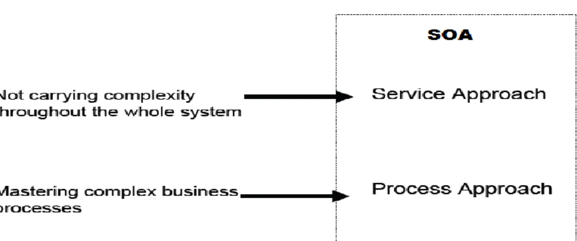
There are 2 main reasons to choose SOA;

Figure 3-Why SOA?

Service approach provides to:

 Integrate sub-systems through services

 Ease uniqueness principle avoiding redundancies

 Build a core framework of services for future development

Process approach provides to;

 Separate business process from code

 Provide better visibility on business processes

(32)

29 5.2 Evolution of Service Oriented Architecture

In the past, programmers had coded little units with a code pieces and system used these code pieces in lots of positions. In old years, it was enough for people to do their work. According to development of new technologies these methods became unserviceable.

In recent years, new communication age damaged the component based architecture. Programmers wanted to use the components of system at the remote machines. This idea exposed new software concepts. These are Distributed Component Object Model (DCOM) and Component Object Model (COM+).

After distributed systems are used, programmers coded little code pieces and put them into only one place to use. So, lots of applications used only one component. This procedure formed the application server.

The usage of software services continued to develop itself day by day. But there was another problem: The coded component runs only on platforms of the same type. Different type of platforms caused many problems. SOA developed to take up this problem to serve best service to users.

5.3 How is Service Oriented Architecture different?

For understanding the difference of SOA from other approaches; first we have to understand its structure. Once the structure is understood it is possible to compare SOA and other approaches to understanding and organizing Information Technology assets.

(33)

30

According to Matthew MacKenzie, Ken Laskey, Francis McCabe, Peter F Brown, Rebekah Metz, Booz Allen Hamilton17 “SOA reflects the reality that ownership boundaries are a motivating consideration in the architecture and design of systems.

This recognition is evident in the core concepts of visibility, interaction and effect. However, SOA does not itself address all the concepts associated with ownership, ownership domains and actions communicated between legal peers.”

The service descriptions and service interfaces inside SOA automatically provide location references. This facilitates the reuse of frameworks and synergic systems which are developed externally.

Additionally, SOA helps applying the lessons which are learned from commerce to the organisation of Information Technology assets for facilitating the matching of facilities and necessities. Thus, entities which league together inside the context of a single interaction require the swap of some type of value.

According to Matthew MacKenzie, Ken Laskey, Francis McCabe, Peter F Brown, Rebekah Metz, Booz Allen Hamilton[22] “This is the same fundamental basis as trade itself, and suggests that as SOAs evolve away from interactions defined in a point-to-point manner to a marketplace of services; the technology and concepts can scale as successfully as the commercial marketplace.”

We will see the effects of SOA on cost estimation in section 7.

17

OASIS-Matthew MacKenzie, Ken Laskey, Francis McCabe, Peter F Brown, Rebekah Metz, Booz Allen Hamilton; “Reference Model for Service Oriented Architecture 1.0”, Committee Specification, 2006

(34)

31

6. ADAPTATION OF SOFTWARE COST ESTIMATION FOR SOA

PROJECT

Today, most companies ask the question “How much this SOA will cost?” for their projects. This is an important question to obtain the funding of the company.

Obtaining the cost of the project is starting with understanding the domain. Understanding the domain in detail includes;

 Number of Data Elements

 Complexity of Data Storage Technology

 System Complexity

 Service Complexity

 Process Complexity

 New Services needed

 Enabling Technology

 Applicable Standards

 Potential Risks

After this step we have to make a decision about required resources for the project and understand their cost.

(35)

32

6.1 Number of Data Elements & Complexity of Data Storage Technology

Defining a unit of data for processing directly effects the project cost estimation while you are creating the data structure of the system.

According to David Linthicum who is an internationally known application integration and service oriented architecture expert, this formula may help to find the data complexity depending on the number of data elements. 18

(8) (8)

The expression is given in Equation (8) is Cost of Data Complexity Equation where;

Number of Data Elements being the number of semantics you are tracking in your domain, new or derived.

Complexity of the Data Storage Technology, expressed as a percentage between 0 and 1 (0% to 100%).

Labor Unit, the amount of money it takes to understand and refine one data element Clearly, if the number of data elements increases then the complexity of the structure will increase as well.

6.2 System Complexity

System complexity is a composite measure of complexity inside procedures and between them. It measures the complexity of a system design according to procedure calls, data use and parameter passing.

18

http://www.soainstitute.org/,David S. Linthicum; “How much will your SOA cost?”, 2007

Cost of Data Complexity = (Number of Data Elements) * (Complexity of the Data Storage Technology) * (Labor Units)

(36)

33

The complexity of system is basically a time and design metric. Before the original implementation exists it is possible to measure the difficulty of creating a designed system.

Also, source code is another important factor for calculating system complexity. It is another way of calculating the complexity of the system.

According to Card and Agresti; 19 “System complexity is not suitable for the evaluation of how difficult it is to change an existing system”.

System complexity contains two main metrics inside it. These metrics are structural complexity and data complexity. We can use these two main metrics while we are calculating the System Complexity.

Figure 4- System Complexity and its metrics

Now, we will see how to calculate system complexity according to the structural complexity and data complexity.

6.2.1 Structural Complexity

Structural complexity is measured by the number of procedures. Structural Fan-in and Fan-out values vary the complexity result directly.

19

Card, D. N. and W. Agresti, "Measuring Software Design Complexity." The Journal of Systems and Software 8, 3; 185-197. (Original definition of the metric),1998

Structural Complexity

Data Complexity

(37)

34

Structural fan-in (SFIN) and fan-out (SFOUT) values are used to evaluate the interrelations between procedures and files. It is also possible to measure the complexity of the static structure of code which includes design and time factors.20

Figure 5- Simple call tree for one procedure

As you see in Figure-5, there are two coming calls to the procedure and when you control the SFOUT we can say that the procedure calls four other procedures to run in the system.

If you think there is more than one procedure in the system, the complexity of the structure will increase according to the SFIN and SFOUTs.

SFIN might be zero thus that means no procedure callers were found in the system. Being too many SFINs are not as desirable for a file.

6.2.2 Data Complexity

Data refers to a collection of information or

facts

usually collected as the result of

experience

,

observation

or

experiment

, or processes within a computer system, or a set of

premises

. For instance, data may consist of numbers and words.

20

(38)

35

Reading and writing business data in some form or order is the main responsibility of e-business applications. So, the storage, management and retrieval of the data always have been a tough problem in all organizations.

Using different mechanisms increases the cost of data depending on the usage of multiple databases.

According to SYS-CON Media’s research 21 “Companies may have heterogeneous data environments with different schemas and they may contain redundant data elements. This data may be static reference data, such as personal customer information or geographical data, common business data, or common external data such as market data. This can lead to serious inefficiencies and consequently higher costs because of the overhead in accessing/updating data in multiple databases using different mechanisms.”

There are some problems that affect the cost estimation of the SOA via data complexity.

These problems may be described as followed;

 Updating the data in multiple channels

 Difficulty of creating a common data spreading strategy for different technologies.

 Data may need to be synchronized between data repositories

 The requirements of the data access performance are increasing through the developing nature of business.

 The diversion of needs and usage patterns of data across systems

Data complexity directly affects the cost of project because of the time factor. If the user spends much more time than usual this means the structure of SOA is not work well. So, we have to develop a scalable strategy that can accommodate new applications with minimal turnaround time.

On the other hand, data has multiple channels of update. Hence, data has to be modified and controlled to make sure that updates are performed regularly.

21

(39)

36 6.3 Service Complexity

Service is the work done by one person or group that benefits another people. The service complexity is related with the size of the project. The services that are given to the customers can be measured by all processes that are served in the system. There might be several factors that affect the service complexity. We can say that, security is one of the main metric of the service complexity.

Today, companies want to provide a secure system service for their customers. So, if the security of the services increases the service complexity may increases as well.

6.4 Process Complexity

Process Complexity is another factor while calculating cost estimation of the system.

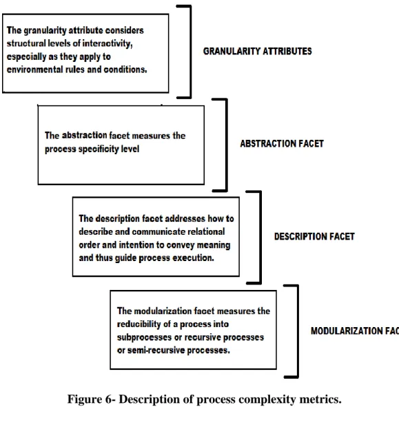
There are some metrics of the process complexity:

 a contents facet including coverage and granularity attributes

 an abstraction facet

 a description facet including form and notation attributes

 a modularization facet22

Figure 6 shows the description of these metrics:

22

C. Roland, “A comprehensive view of process engineering, Proceedings of the 10th international conference ” and B. lecture notes in computer science, Italy, 1998

(40)

37

Figure 6- Description of process complexity metrics.

6.5 New Services

Services are changing day by day. Thus, companies should be able to give new services to their customers to address much more people.

New technologies provide to add new customers to use your system. Needless to say that, adding new customers to the system takes some time. Increasing user number means the company of yours can earn much more money.

New standards bring new cost to your company and it is hard to raise the price of the services. This problem may be solved by reducing the operating costs.

(41)

38

According to the description above, by understanding the needs of your users, you can manage the cost of your system and give better service to customers. Otherwise, the cost of the system may increases.

6.6 Enabling Technology

Enabling technology is another metric for understanding the domain. Developing the domain of the system by using new technologies may decrease the development time of the project. So, the cost of the project will be decreased automatically.

6.7 Potential Risks

Beside all of these factors, we should think about risks during the project development. For example, economic crisis, decrease of the developer performance or problems during analysis process. Especially, analysing process takes too much time because of the misunderstanding between analyser and customer.

Unfortunately, most companies do not care about analysing process as much as it needs. Because, the manager of the project thinks that it is a loss of time to analyse deeply and they want to start development process immediately. However, analysing process is the main factor of the cost estimation.

Disregarding the analysing process may cause more loss of time unlike the manager’s thinking. Therefore the risk of project might be increased.

Project risk is considered low when all processes involve fairly simple operations. Project risk is considered medium when the minority of the business processes under automation is complex, involving multiple steps, exchanges with external systems or significant validation/processing logic. Project risk is considered high when a majority of the business processes under automation are considered to be complex.

(42)

39

7. A NEW POINT OF VIEW TO SERVICE ORIENTED

ARCHITECTURE COST ESTIMATION

The business conditions are changing day by day. SOA is developed to make IT more flexible. By using SOA, IT becomes adapted to changing business conditions.

SOA provides some advantages like simplifying integration, managing complexity, reducing costs and increasing reuse. As we mentioned, SOA is directly related with cost.

Steghuis 23gives useful major reasons to answer the question “Why SOA is better in reducing costs?” These are:

 SOA implies a services mind-set and this anticipates shared use of services.

 SOA leads to monitoring and management of quality of the services so that experiences of the shared services can be exchanged.

 Services encapsulate complexity and isolate changes by only exposing their interface to the outside world.

 Standardisation of interfaces and the way they are exposed reduces cost and promotes reuse

 Services architecture focuses on the end-to-end lifecycle instead on single lifecycle stages.

On the other hand service granularity of SOA affects the whole system by changing its complexity. "Service granularity is the scope of functionality exposed by a service". [41]

23

(43)

40

Modularity of a system can be reflected by its granularity. SOA needs to have well designed services to provide flexible business processes. Well-designed services provide low development cost.

Now, we can explore component based SOA systems to adapt new cost estimation facilities into SOA cost.

(44)

41

8. GENERAL VIEW OF COMPONENT BASED SOA SYSTEMS

8.1 Step by Step Cost Estimation in Component Based SOA Systems

Component based system is a branch of software engineering. This system consists of components that include data and functions inside it. These components are modular and cohesive, because they are semantically related with the contents of classes.

Each component may offer services from the system. The whole system finds the related interface that is offered by the component. We can say that interfaces are the signatures of related components. They find the services that will be used by the component. Component can use other component by using their interfaces.

While designing Component-Based System; first of all, we have to define the requirements of the system. These requirements help to generate the components of the system.

During planning the structure of the system, we should find new ways to make it flexible for using it in different platforms.

Decomposition of requirements is one of the most important processes before finding function points for each component. Because, using a lot of unnecessary components means much more line of code. So, it may affect the cost of the system. To determine complexity; for each component, we have to find Function Point items to calculate the cost estimation of service.

(45)

42

As we said before, we have to find external inputs, external outputs, logical internal files, external interface files and external inquiries to determine the complexity of the system.

If the number of components of the system increases than the UFP (Unadjusted Function Point) will increase as well. Function points will be affected by the value of UFP and technical factors. Technical factors are the total number of factors that affect the technical complexity.

UFP can be used to find the line of code. Line of code is the value that affects the cost of the system. Line of code will increase if the UFP increases. So, we have to compose the components of the system carefully.

Before determining the complexity of system, we will see how to decompose the SOA.

8.2 Evolution of Decomposition in Software

According to Boris Liblinsky; the first software decomposition approach introduced in the early 1960s was splitting mainframe applications into separate jobs, each implemented by a separate program. Later, as more insight into the program internals was gained, each program itself was split into modules or subroutines, according to their function.24

In 1970’s decomposition adoption by introducing objects strengthened. These objects was implemented a model of real thing. Bust, on the other hand, abstractions provided by objects turned out to be too fine grained to have meaning on business level.

(46)

43

To find better designed paradigm, researchers continued searching to find different approaches to decomposition in the late 1990’s. Researchers were thinking that raising the level of abstraction and increasing granularity will help to fix the problems of object oriented systems.

According to component based architecture, software applications were much more flexible, better structured and more manageable. But, on the other hand it was decomposing the enterprise IT functionality.

(47)

44

9. APPLICATION SIZE USING FUNCTION POINT ANALYSIS

(FPA)

Function point analysis (FPA), is one of the most popular and usable approaches for estimating the software size.

There are three main processes of FPA. These are;

 It quantifies the functionality requested by the customers and also provided functionality to the customers.

 Measure software development and maintenance independently of technology used for implementation.

 Across all projects and organizations, consistently measures the software development and maintenance.

User’s view of the system can change the size of the project according to their requirements. The inputs, reports, screens, stored data on the system will change the size of the application. We can say that user interactions may be one of the important inputs to change the size estimation of system.

FPA does not matter if it is an application written in .Net, Java etc… It is technology independent.

Adding FPA to our system is not expensive and provides to measure the size of the project to calculate the cost estimation of the system. FPA well works with use cases, so it is useful for object oriented software as well.

(48)

45

FPA measures the cost, duration, staffing size of the project. It seems to be easy to understand Cost per FP, FP’s per hour and project defect rate metrics by using FPA.

The benefits of PFA are,

 Difficulties of estimation using Lines of Code can be avoided by using function point analysis.

 Sizing is important while determining the productivity of the system. FPs can be used to size software applications accurately.

 FPA is easily understood by every people, so it helps communicate sizing info to a user or customer.

 FPA is more productive than other methods, because it can be used to determine whether an environment, tool and language.

 The time or person is not important, they can be counted by different people at different times and they obtain the same measure within a reasonable margin of error.

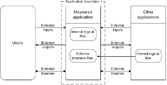
Thomas Fetcke, Alain Abran and Tho Hau Nguyen25 have used “o-o Jacobson Approach”. Figure-8 gives details about their function model.

Figure 8- A high Level view of the abstract function point model with users and links to other applications.

25_{Thomas Fetcke, Alain Abran and Tho Hau Nguyen, “Mapping the o-o JacobsonApproach into}

(49)

46

9.1 Data Functions and Transactional Functions

As we mentioned in function point section; there are five main functions to be counted. Two of them are data functions and the other three are the transactional functions.

Figure 9- Data Functions and Transactional Functions

Using this terminology one of the researcher has drawn a figure to understand counted metrics during FPA.26

Figure 10- View of a software application from the eyes of a Function Point practitioner.

26_{Alvin J. Alexander; “How to Determine Your Application Size Using Function Point Analysis”,}

(50)

47 9.1.1 Data Functions

(i) Internal Logical Files (ILF)

ILF represents the data stored in the system. For counting ILF we have to make sure that the data and group information are logical and user identifiable.

The group of data which is maintained through the beginning operation should be counted. Tables in a database and flat files can be an example to the ILFs.

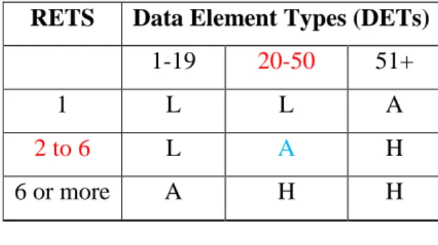
First of all we have to determine the complexity level of Low (L), Average (A), or High (H). We can do this by counting number of Data Element Type (DET) and Record Element Type (RET).

RET is user recognizable data elements within ILF and EIF (External Interface File).DET is a unique, user recognizable and non-repeated field. You can find the points by complexity by checking number of DETs and RETs.

RETS Data Element Types (DETs)

1-19 20-50 51+

1 L L A

2 to 6 L A H

6 or more A H H

Table 1- ILF complexity matrix

For example, according to Table-1, we can say that, if there are 4 RETs and 25 DETs then, that system would bear (A) Average Complexity. This example is based on a real time project which is found on the internet.

(51)

48

Table 2 - ILF Complexity Matrix Weight.27

As you can see in table 2, a Low complexity ILF is worth 7 points, an Average ILF is worth 10 points, and a High is worth 15 in their example.

After finding complexity from the complexity table, we can determine the number of FPs that will be counted for this ILF. According to our example, the complexity is

Average, so we can say that, the function points of this ILF will be 10FPs.

(ii) External Interface Files (EIF)

EIF represents the data that the application will use or refer. These data cannot be maintained by the existing system.

The main difference between EIF and ILF is that the EIF uses data maintained within the boundary of another application. ILF uses its own application. The data is not maintained within the boundary of another application. You can find the points by complexity by checking number of DETs and RETs.

As we mentioned on ILF section, checking the number of RETs and DETs will help us to find complexity and weight of the application. According to the tables above you can check the values and calculate complexity and weight.

27 http://www.devdaily.com Complexity Points Low 7 Average 10 High 15

(52)

49

RETS Data Element Types (DETs)

1-19 20-50 51+

1 L L A

2 to 6 L A H

6 or more A H H

Table 3- EIF Complexity Table [27]

According to the table-3, we can say that, if we count 3 RETs and 21 DETs that would be of (A) Average Complexity.

Table 4- EIF Complexity Matrix Weight [27]

According to our example, the complexity is Average, so we can say that, the function points of this ILF will be 7 FPs.

We found real examples which are really useful to understand the transactional and data files. 28

Now we can consolidate the information about External Interface Files (EIF). Assume that our system goes to another boundary to find and take a Zip/Postal Code then gets full address detail from another system and fills our address detail fields automatically. You can find these examples in Figure 11 and Figure 12.

28 http://www.softwaremetrics.com/examples/ Complexity Points Low 5 Average 7 High 10

(53)

50

Figure 11- EIF example Part-1: The service goes to another boundary to find and take a Zip/Postal Code.

Figure 12- EIF example Part-2: The service takes Zip Code and states City and State fields automatically.[27]

In this example, we can see the combined effect of an EQ and EIF.

Here, External Inquiry has 3 DETs. These are zip code, city and state fields.

It references just one FTR. Zip code field is an EIF, because it uses another application boundary. Now, we can say that the complexity of this EIF is Low and it points to 5 unadjusted function points.

(54)

51

Every EIF must have at least one transaction against it. Also, one of the EI, EO and EQ should refer to EIF.

9.1.2 Transactional Functions

According to Thomas Fetcke, Alain Abran and Tho Hau Nguyen29 “There can be a one-to-one, one-to-many or many-to-many relation between deliverables visible to the user and transactions”. Before describing transactional functions, it would be better to understand the Figure-13 of these researchers.

Figure 13- Identification of items within the counting boundary. (i) External Inputs (EI)

External input processes data or control information which comes from outside the boundary of an application. Data entries and data or file feeds by external applications can be an example to the EI.

To find the complexity of the application we have to determine the DETs and FTRs (File Type Referenced). FTR can be either ILF or an EIF.

FTRs Data Element Types (DETs)

1-4 5-15 16+

0-1 L L A

2 L A H

3 or more A H H

Table 5- EI Complexity Table [27]

29_{Thomas Fetcke, Alain Abran and Tho Hau Nguyen, “Mapping the o-o JacobsonApproach into}

(55)

52

For example, according to the table-5, we can say that, if we counted 4 FTRs and 12

DETs that would be a (H) High Complexity.

Table 6- EI Complexity Matrix Weight [27]

After finding complexity from the complexity table we can determine the number of FPs that will be counted for this EI. According to our example, the complexity is

High, so we can say that, the function points of this EI will be 6 FPs.

We can give another example to consolidate the information about External Inputs. Here is an interface that shows Address Info page on the application.

Figure 14- EI example [27] This external input shown in Figure-14,

 Rated as a low EI  Valued at 3 unadjusted FPs  FTR is 0 Complexity Points/Weight Low 3 Average 4 High 6

(56)

53

 And has 15 Data elements(DETs) that create one ILF.30 You can confirm the complexity is low by checking Table-5.

According to this example, we have to know that each field that is saved or invokes the transaction will be counted as a data element. We can say that it is an External Input which has 15 Data elements(DETs) that create one ILF.

The OK button here will be counted as a DET. After using OK button, all information will be saved in an ILF file. Now we have a little more information about EI, DEF and ILF.

(ii) External Outputs (EO)

External output is a beginning process that sends data or control information outside the application boundary. According to the International Function Point Users

Group’s research 31

“reports created by the application being counted, where the reports include derived information can be an example to EO.”

Allocating FPs to EOs is very similar to the process for EIs.

To find the complexity of the application we have to determine the DETs and FTRs (File Type Referenced) as an EO process.

1-5 6-19 20+

0-1 L L A

2-3 L A H

4 or more A H H

Table 7- EO Complexity Table [27]

For example, according to Table-7, we can say that, if we counted 0 FTRs and 1

DETs that would be a (L) Low Complexity.

30_{http://www.softwaremetrics.com/examples/ei.htm} 31

(57)

54

Table 8- EO Complexity Matrix Weight [27]

According to our example, the complexity is Low, so we can say that, the function points of this EO will be 4 FPs.

Now, we can consolidate the information about External Outputs by giving a real example. This is a 3 data elements (DET’s) interface. Also it references 4 FTR's (file types referenced) and would be rated as an Average and valued at 5 unadjusted function points.32 You can confirm the complexity Average by checking Table-8.

Figure 15- EO example [27]

We can say that, the Amount column is a derived data. It is not stated on FTR. Description and Due date data elements can be found on FTR. According to this information we can say that, External Outputs are the calculated data.

The due date does not take apart in this example. So, the due date counted as a DET here. 32 http://www.softwaremetrics.com/examples/eo.htm Complexity Points/Weight Low 4 Average 5 High 7

(58)

55 (iii) External Inquiries (EQ)

According to the description of the International Function Point Users Group [30]“An external inquiry (EQ) is an elementary process that sends data or control information outside the application boundary”.

To find the complexity of the application we have to determine the DETs and FTRs (File Type Referenced).

Table 9- EQ Complexity Table [27]

For example, according to the table-9, we can say that, if we counted 3 FTRs and 15

DETs that would be a (A) Average Complexity.

Complexity Points/Weight

Low 3

Average 4

High 6

Table 10- EQ Complexity Matrix Weight [27]

According to our example, the complexity is Average, so we can say that, the function points of this EQ will be 4 FPs. Now, we will consolidate the information about External Inquiries by giving a real example.

1-5 6-19 20+

0-1 L L A

2-3 L A H

Software cost estimation in the soa age

SOFTWARE COST ESTIMATION

IN THE SOA AGE

SOFTWARE COST ESTIMATION

IN THE SOA AGE

ASLI YILMAZ TAġKIN

Abstract

Özet

Acknowledgements

Table of Contents

List of Tables

List of Figures

1. INTRODUCTION

2. GENERAL VIEW OF SW COST ESTIMATION

3. COCOMO&COCOMO II COST ESTIMATION MODELS BY

USING COSTAR AND FUNCTION POINTS

4. PRINCIPLES OF THE COCOMO CALCULATION

(1)

(3)

LOC= a* UFC +b

W

N

n

UFC

Σ Σ

N

W





*

W

n

UFC

FP=UFP x (0.65+0.01xTCF)

TCF



C



C

F



5. INTRODUCTION TO SERVICE ORIENTED ARCHITECTURE

6. ADAPTATION OF SOFTWARE COST ESTIMATION FOR SOA

PROJECT

facts

experience

observation

experiment

premises

7. A NEW POINT OF VIEW TO SERVICE ORIENTED

ARCHITECTURE COST ESTIMATION

8. GENERAL VIEW OF COMPONENT BASED SOA SYSTEMS

9. APPLICATION SIZE USING FUNCTION POINT ANALYSIS

(FPA)