TARIM BILIMLERI DERGISI 2001, 7 (4) 121-128
An Application and Interpretation of the Second Order
Response Surface Model
Zahide KOCABAŞ° Geli
ş Tarihi : 14.09.2001
Abstract: In this study, three artificial data sets were used to explain the second order response surface model. It was assumed that the data were collected from a 3x3 experiment with two replications. Fitting the second order response surface model showed that 92.51%, 83.93% and 85.41% of the tatei variation in YIELD1, YIELD2 and YIELD3, respectively, accounted for by the fitted model. When the lack of fit test was applied, the results clarifıed that the second order model was adequately described the response surface for all the three sets of data. Application of the canonical analysis confırmed that there was a stationary point of maximum response for YIELD1, a stationary point of minimum response for YIELD2 and a saddle point for YIELD3. After that, the data on the corrected sugar content of sugar beet were analyzed. The results showed that the fitted second order model accounted for 68.9% of the total variation in the sugar content. When the lack of fit test was applied, the results showed that the second order model adequately described the response surface of sugar content. The results of canonical analysis indicated that there was a saddle point for the sugar content.
Key Words: Response surface, second order model, stationary point, saddle point, maximum point, minimum point
İ
kinci Derece Yan
ı
t Yüzey Modellerinin Uygulamas
ı
ve Yorumlanmas
ı
Özet: İkinci derece yanıt yüzey modellerinin uygulaması ve sonuçların yorumlanması için yapay olarak oluşturulan üç veri kümesi kullanılmıştır. Verilerin 3x3 düzeninde tertiplenmiş iki tekerrürlü bir denemeden toplandığı varsayılmıştır. Yapay olarak oluşturulan veriler için ikinci derece yanıt yüzey modeli hesaplandığı zaman VERIMI 'deki toplam varyasyonun %95.52'sinin, VERİM2'deki toplam varyasyonun %83.93'ünün ve VER İM3'teki toplam varyasyonun %85.41'inin hesaplanan model tarafından açıklandığı görülmüştür. İkinci derece modelin uygunluk kontrolünden elde edilen sonuçlar hesaplanan modelin yanıt yüzeyini tanımlamak için yeterli olduğunu göstermiştir. Yanıt yüzeyinin yapısını incelemek için uygulanan kanonik analiz VERIMI için maksimum, VERİM2 için minimum olduğunu göstermiştir. Buna karşın VERİM3 için bir eyer (saddle) noktası hesaplanmıştır. Yapay veriler kullanıldıktan sonra şeker içeriğine ait toplanmış veriler analiz edilmiştir. Şeker içeriği verileri için ikinci derece yanıt yüzeyi modeli hesaplandığı zaman, şeker içeriğindeki toplam varyasyonun %68.9'unun hesaplanan model tarafından açıklandığı görülmüştür. İkinci derece modelin uygunluk kontrolünden elde edilen sonuçlar hesaplanan modelin şeker içeriği için yanıt yüzeyini tanımlamak için yeterli olduğunu göstermiştir.Uygulanan kanonik analizde şeker içeriği için bir eyer (saddle) nokta hesaplanmıştır. Anahtar Kelimeler: Yanıt yüzeyleri, ikinci derece model, kritik nokta, eyer noktası, maksimum ve minimum nokta
Introduction
Response surface methodology (RSM) includes mathematical and statistical techniques. The techniques incorporated in the RSM are useful for modeling, analyzing and optimizing processes. There are two kinds of variables in this methodology. One of these is the performance or quality characteristic, which is called the response variable. The application of RSM can generally involve more than one response. The other one is the input variable, which is commonly called independent variable and is subject to control. RSM is used to inspect the relationship between one or more response variables and a set of independent experimental variables.
The main purpose of RSM is to determine the ievels of independent variables that produce the best response. Response surface methods are also employed to fit a suitable function to be used for the aim at predicting future response. Moreover, the RSM enables the researcher to identify new operating conditions that produce desired improvements.
The RSM is extensively used in many areas for different objectives. The response surface methods were performed to optimize the diced tomato calcification process by Fioros et al. (1992). They evaluated the effects of calcium concentration, temperature of dipping solution, and contact time on calcium uptake, firmness and pH of diced tomatoes during a calcification process using response surface methods. Pereira et al. (1992) conducted an experiment to develop a cheese analog containing aqueous soy extract, whey and cow's nnilk by using lactic fermentation and calcium sulfate to obtain a coagulum. They employed the response surface methodology with a 3-3 incomplete factorial design to optimize experimental conditions. Prapulla et al. (1992) carried out an experiment where levels of nitrogen, carbon and inoculum were chosen as factors and used RSM to maximize the lipid production. Agarwal et al. (1994) calculated a quadratic response surface equation for economizing fertilizer use for rainfed sesame crop in Doon Valley. The influence of cutting speed and cutting angle on
'Ankara Univ. Fac. of Agr.
A the energy and peak force requirements for potato slicing
were investigated using an Instron —6201 universal testing machine by Kulshreshtha et al. (1988). They analyzed the observed data by using RSM. Castro et al. (1998) applied statistical response surface methodology to determine the proportions of 3 protein substrates that could be incorporated into a formula for a chocolate milk drink to reduce the costs without causing signiflcant changes in sensory properties. It is too possible to give examples on the use of RSM in different areas in the literature.
This study was attempted to exhibit the applicability of the second order response surface model, the interpretation of the results and the problems to be encountered. For this purpose, first three artificial data sets were used to give details on the application of RSM, the elucidation of the results and the problems to be met. After that, the information gained from the application of RSM to the artificial data was applied to the real sugar beet data. In this way, the impediments and questions to be met in practice were discussed and solutions to these situations were recommended.
Material and Method
First artifıcial data were used in this study. In artifıcial data sets, it was assumed that there were three levels of Factor A (5, 10 and 15) (FA) and Factor B (5, 10 and 15) (FB) and that the experiments were full factorial in randomized design with two replications. In these experiments, the assumed response variable was yield. (The response variable was represented as YIELDI for the first set of data, YIELD2 for the second set of data and YIELD3 for the third set of data).
After that, the data collected from the experiment carried out in Konya in 1998 were used. The purpose of the experiment was to investigate the impacts of the different N-levels and sowing dates on the quality of sugar beet. In the experiment, seven levels of N (4, 8, 12, 16, 20, 24 and 28 kg /da) were examined with two sowing dates (early (15 April) and late (30 April) sowing) in a factorial design with six replications. The data on the corrected sugar content were used as response variable in this study.
Suppose that there is an experiment involving a response variable, y, depending on the controllable input variables In this case, the relationship between the y and input variables can be expressed as
Y=f( ı , ...(1)
where the form of the function f is unknown, E ıs the error term that represents the variability that cannot be accounted for by f. The variables in equation (1) are called natural variables and expressed in the natural units of measurements, such as kg/da. In RSM work, it is convenient to transform the natural variable to coded variables, x1, x2, x3, ..,xk that are usually expressed as dimensionless. In terms of the coded variables, the equation (1) can be written as
Ti=f(xı, x2, x3,...,xk) ....(2)
. It is convenient to choose the level of to be equally spaced because there is no restriction on choosing the levels. The relationship between the and xu can be expressed as:
- ( 3 )
where is the mean of and A is the difference in the levels of
In most cases, the first order response surface model adequately describes the response y as a function of input variable. However, if there is a curvature in the response surface, the first order response surface model will be inadequate. In these situations, a second order response surface is required to constitute a suitable function. The second order response surface model for the case of two variables is written as
E(y) = 130 + + E Piixi2 +13. xix, + E ... (4)
i=1 1=1 ki '
where 130, J3ı and xi are as for the first order polynomial model, 13ii is the second order coefficient for the ith variable, f3d interaction coeffıcient for the interaction of variables i and j and s is the error term.
The estimating equation can be written, in matrix form, as: in which X = = - x 1 x 2 x 3 x k bo b= + x'b b1 b 2 b 3 b k + x'Bx • • ( 5 ) b 11 )/ 2 ... (b lk)/ 2 b 22 (b2k )/ 2 symm b kk
where b is a (k x 1) vector of the linear regression coefficients and B is a (k x k) symmetric matrix with quadratic regression coefficients (bii) in the diagonal elements and orıe-half the mixed quadratic regression coefficients (b,, in the off-diagonal elements.
x
İ
J
. =
5
- oy
KOCABAŞ, Z. "An aplication and interpretation of the second order response surface model" 123
In some cases, it can be required to involve the other terms, for example, x1 2x2, x1x2 , 2 2 x22 i• n the case of two
variables, to obtain an adequate function to describe the true response surface. But, these terms are generally ignored and are included in the sum of squares of lack of fit.
The parameters of the model are estimated by least squares regression. In this way, information on the fit in the form of an analysis of variance is obtained. The sum of squares of lack of fit is calculated as the difference between treatments sum of squares and the regression sum of squares. This sum of squares is the measure of the failure of the treatments means to conform to the second order model in xı, x2. If the lack of fit is not signifıcant, it can be possible to estimate the parameters in equation 5.
Having tested the second order model, the next step is to analyze the response surface to find the points at which
9
is a minimum or maximum. To do this,9
is differentiated with respect to each x, in turn, equated to zero and solved for xo, the coordinates of a point in x1, x2.xk. This calculated point might be minimum, maximum or saddle for
9.
This point is called stationary point because it is the point at which the rate of change is zero.A general mathematical solution for the location of the stationary point can be obtained by writing the equation 5. The derivative of
9
(eq. 5) with respect to the elements of the vector x equated to zero is written as:—
öç( = b+2Bxöx
... (6)
The stationary point is to solution to equation 6 or
xs =
1
B
_
1
b
•-(7)The predicted response at the stationary point is giyen as:
Having calculated the stationary point, it is required to inspect whether the stationary point is a point of maximum, minimum or a saddle point.
The fitted response surface can be expressed by writing the following equation:
9=9 s +Aiw.,
2
+A 2 w
2
2 +...+A k w,
2
....
(9) where, wi are the transformed independent variables and >ı are constants which are just the eigen values or characteristic roots of the matrix B. In other word, the eigen values X.1 and 9,.2 are the roots of the determinantal equation of IB-X.11=0. The equation 9 is called the canonical form of the model. If the X, are all positive, then xs is a point of minimum response, if the X are all negative, then xW is a point of maximum response, rf the have different signs, xs is a saddle point. The negative eigen values indicate the directions of upward curvature. Whereas, the positive eigen values indicate the downward curvature (Petersen 1985, Myers and Montgomery 1995, Montgomery 1997).Results
The artificial data sets are separately analyzed in order to explain a point of minimum or maximum response, or a saddle point. These artificial data are supposed to be collected from an experiment in which the impacts of FA and FB on yield were examined in a full factorial design with two replications. The treatments include 3x3 factorial combinations of FA and FB, where FA=1 and FB=.2. The design variables, xı, for FA and x2i for FB were obtained by the following transformation:
The resulting design points and yields (kg/da) are giyen in Table 1. The ANOVA was applied to the data. The results of this analysis are giyen in Table 2.
y
13
s
=b0+-1
;s
2
...( 8)Table 1. Design points and yields for a 3x3 experiment (Rep: Replication, Trts: Treatments )
Trts. Design points Natural variables YIELD1 YIELD2 YIELD3
X1 X2 FA FB Rep1 Rep2 Rep1 Rep2 Rep1 Rep2
N Lr) N o o o ı r ı 11,
J
5 5 7 16 14 10 9 10 9 8 8 7 8 12 15 7 8 23 26 11 13 5 10 10 8 10 8 9 O O 10 16 18 6 7 13 11 15 14 16 12 10 9 10 5 7 6 21 23 17 18 10 11 10 23 32 15 19 15 12 12 30 45 16 1718 17 18 15 14 13 YIELD3 12 ıı ıo e
Figure 1. Response surface plot of YIELD1
Figure 2. Response surface plot of YIELD2 Table 2. The result of ANOVA for YIELD1 , YIELD2 and YIELD3
Source of variation Degrees of freedom Mean of squares YIELD1 YIELD2 YIELD3 X1 X2 X1*X2 Error N N • st C» 88.87" 36.50- 4.42* 0.8g 631.17- - 193.50 42.67 18.50 91.50- 2. 17 4.17 2.50 .P<0.05, P<0 01
As seen in Table 2, the interaction between X1 and X2 is statistically significant for YIELD1. The difference in yield amongst the levels of X1 is significant for all data sets. However, there is the evidence that there is a statistically significant difference in yield amongst the levels of X2 for YIELD1 and YIELD2.
In the case of two variables with three levels, a response surface model can include 8 terms that are xı, X2, Xi2, X22, XiX2, Xİ2X2, X1X22 and xi-2 x22 If regression analysis is applied and the sum of squares caused by each of these terms are calculated, it can be seen that the sum of squares of X1 in Table 2 equals to the sum of squares of xi and x12. Similarly, the sum of squares of X2 in Tables 2 equals to the sum of squares of x2 and x22. The sums of squares caused by the remaining 4 terms constitute the sum of squares of interaction. However, as mentioned before, xi2x2, xix22 and xi2x22 are ignored and they are included in the sum of squares of lack of fıt. In order to show this situation, the sum of squares caused by each term was calculated and the results are giyen in Table 3.
As seen in Table 3, the total of the sum of squares of xi (16.333) and xı2 (121.000) equals to the sum of squares of X1 in Table 2. The sum of squares of X2 is constituted by x2 (48.000) and x22 (25.000). The sum of squares caused by the remaining terms forms the sum of squares of interaction.
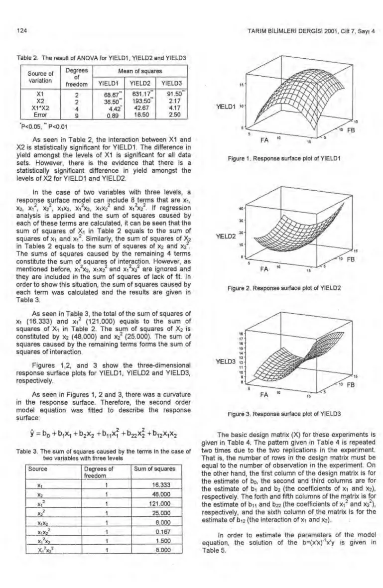
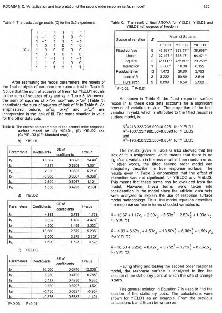
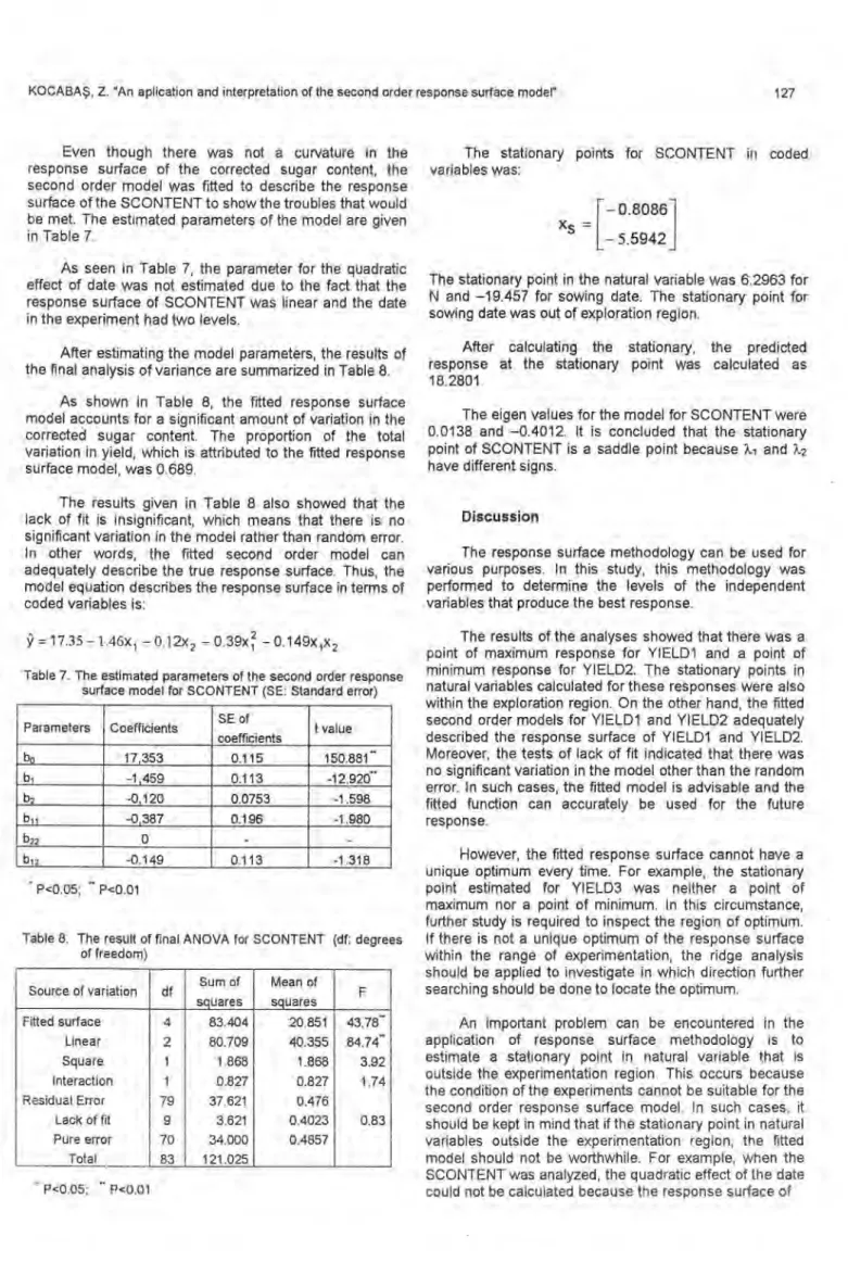
Figures 1,2, and 3 show the three-dimensional response surface plots for YIELD1, YIELD2 and YIELD3, respectively.
As seen in Figures 1, 2 and 3, there was a curvature in the response surface. Therefore, the second order model equation was fitted to describe the response surface:
9
=bo
+b
2
x2+b
11
x12 ±b22X22+b
12 X1 X2
Table 3. The sum of squares caused by the terms in the case of two variables with three levels
Source Degrees of freedom Sum of squares x1 1 16.333 X2 1 48.000 X1 2 1 121.000 x22 1 25.000 X1X2 1 8.000 x1x22 1 0.167 X1 2 X2 1 1.500 X1 2x22 1 8.000
Figure 3. Response surface plot of YIELD3
The basic design matrix (X) for these experiments is giyen in Table 4. The pattern giyen in Table 4 is repeated two times due to the two replications in the experiment. That is, the number of rows in the design matrix must be equal to the number of observation in the experiment. On the other hand, the first column of the design matrix is for the estimate of bo, the second and third columns are for the estimate of bi and b2 (the coefficients of xi and x2), respectively. The forth and fifth columns of the matrix is for the estimate of bil and b22 (the coefficients of x12 and x22), respectively, and the sixth column of the matrix is for the estimate of biz (the interaction of xi and x2).
In order to estimate the parameters of the model equation, the solution of the b=(x'x)-lx'y is giyen in Table 5.
KOCABAŞ Z. "An aplication and interpretation of the second order response surface model" 125
Table 4. The basic design matrix (X) for the 3x3 experiment
1 -1 -1 1 1 1 1 -1 0 1 O O 1 -1 1 1 1 -1 1 0 -1 O 1 O X=
1
0 0 O O O1
01
O 1 O1
1
-1 1 1 -11
1
0 1 O O1
1
1
1 1 1After estimating the model parameters, the results of the fınal analysis of variance are summarized in Table 6. Notice that the sum of squares of linear for YIELD1 equals to the sum of squares of xı and x2 in Table 3. Moreover, the sum of squares of x1 2)(2, x1x22 and x1 2)(22 (Table 3) constitutes the sum of squares of lack of fit in Table 6. As emphasized before, )(1 2x2, x1x22 and x1 2x22 are incorporated in the lack of fit. The same situation is valid for the other data sets.
Table 5. The estimated parameters of the second order response surface model for (A) YIELD1, (B) YIELD2 and (C) YIELD3 (SE: Standard error)
A) YIELD1 Parameters Coefficients SE of coefficients t value bo 15.667 0.6395 24.49- b1 1.167 0.3503 3.331 b2 2.000 0.3503 5.710- b11 -5.500 0.6067 -9.066„ b22 -2.500 0.6067 -4.121 bız 1.000 0.4290 2.331 B) YIELD2 Parameters Coefficients SE of coefficients t value bo 4.833 2.718 1.778 b1 6.667 1.489 4.478 b2 4.500 1.489 3.023- bı i 13.500 2.579 5.235... b22 6.000 2.579 2.321 biz 1.500 1.823 0.823 C) YIELD3 Parameters Coefficients SE of coefficients t value bo 10.500 0.8746 12.006- b l 3.250 0.4790 6.785- b2 0.417 0.4790 0.870 b 11 3.750 0.8297 4.52- b22 -0.750 0.8297 -0.904 1012 -0.875 0.5867 -1.491 P<0.05; P<0.01
Table 6. The result of fınal ANOVA for YIELD1, YIELD2 and YIELD3 (df: degrees of freedom)
Source of variation df Mean of Squares YIELD1 YIELD2 YIELD3 Fitted surface In N N ,-.. " c , ) o ı 1 43.667** 333.47** 38.695** Linear 32.167** 388.17** 64.471 ** Square 73.000** 436.50** 29.250** Interaction 8.000* 18.00 6.125 Residual Error 1.472 26.60 2.753 Lack of fit 3.222 50.89 3.514 Pure error 0.889 18.50 2.500 • P<0.05, P<0.01
As shown in Table 6, the fitted response surface model in all these data sets accounts for a significant amount of variation in yield. The proportion of the total variation in yield, which is attributed to the fitted response surface model, is:
R2=218.333/236.000=0.9251 for YIELD1 R2=1667.33/1986.50=0.8393 for YIELD2 and
R2=193.458/226.500=0.8541 for YIELD3
The results giyen in Table 6 also showed that the lack of fit is insignifıcant, which means that there is no significant variation in the model rather than random error. In other words, the fitted second order model can adequately describe the true response surface. The results giyen in Table 6 emphasized that the effect of interaction was not significant for YIELD2 and YIELD3. This means that these terms can be excluded from the model. However, these terms were taken into consideration in the model since the artificial data sets were analyzed to explain the use of response surface model methodology. Thus, the model equation describes the response surface in terms of coded variables is:
9 =
15.67 +1.17x1 + 2.00x2 - 5.50)(12 - 2.50x 22 +1.00x1x2 for YIELD1 2 9 = 4.83 + 6.67xi + 4.50x2 +13.50xi2 + 6.00x 2 + 1.50xix2 for YIELD29 =
10.50 + 3.25x 1 + 0.42x 2 + 3.75x - 0.75x 22 - 0.88x /x2 for YIELD3Having fitting and testing the second order response model, the response surface is analyzed to fınd the location of the stationary point at which the rate of change is zero.
The general solution in Equation 7 is used to find the location of the stationary point. The calculations were shown for YIELD1 as an example. From the previous calculations b and B can be written as
8.8617
8.2673_
8.12311
for YIELD3. for YIELD2 and
12.4838
- 5.5 0.5
0.5 - 2.5
From Equation 7 the stationary point is
1 _
İ
x
s
=--
2
B b
_ _
1/2
[-
0.037011.1671 [0.14511
- 0.0370 - 0.4074 2.000
0.4290
That is, xı.5=0.1451 and x2 5=0.4290. In terms of natural
variables, the stationary point is
- 10
- 10
0.1451 = '
0.4290 =
5
5
which yields = 10.7255 =11 for FA and = 12.145 = 12
for FB.
When the same calculations were done for YIELD2 and YIELD3, the stationary points in coded variables are:
-
0.22771
s -
0.3754
0.4968
f
for YIELD2 and x =
for
x
s [
-0.3465
YIELD3. The stationary points in terms of natural variables are:
After fınding the location of the stationary point, the
predicted response at the stationary point was calculated using Equation 8 as:
10 14511 167 y s = 15.667 +- [
20.42901 [2.000 " = 16.807 for YIELD1,
ys=3.295 for YIELD2 and y 5=9.993 for YIELD3.
The stationary point can be a point of maximum response or minimum response, or a saddle point. In order to investigate whether the stationary point is maximum, minimum or saddle, the canonical analysis is used. First, the fitted model is expressed in canonical form as in
Equation 9. The eigen values Xi and X2 are the root of the
determinantal equation 18-X11=0. This equation for YIELD1 is:
- 5.5 - A
0.5
0.5
- 2.5 - A
which reduces to
X2+ 8X+13.5=0
quadratic equation are Xı=-2.4189 and
these results, It is concluded that the YIELD1 is a maximum because both
and X2 are negative. and the stationary point is within the
examination region.
The analysis of the fitted surface for YIELDI indicated that a maximum yield of 16.807 was obtained at a FA of 11 and at a FB of 12. In other word, if the researcher is interested in investigating the effect of application of N (kg/da) and P (kg/da) on yield and if FA refers to the N and FB refers to the P in the experiment, the maximum yield of 16.807 will be obtained when 11 kg/da of N and 12 kg/da of P were applied.
Similarly, the eigen values for the response surface model for YIELD2 and YIELD3 were calculated. The eigen values for the model for YIELD2 were 13.5743 and 5.9257. It is concluded that the stationary point of YIELD2
is a minimum because both Xı and X2 are positive and the
stationary point is within the examination region.
The analysis of the fitted surface for the YIELD2 pointed out that a minimum yield of 3.295 was obtained at a FA of about 9 and at a FB of 8. In this case, if the factors investigated in the experiment causes yield loss, in anyway, the minimum yield loss occurs at the about 9 of FA and FB of 8. Moreover, the eigen value associated with FB (5.9257) was quite a bit smaller than the eigen value associated with FA (13.5743), which indicates that the response surface was relatively insensitive to the changes in FB.
The eigen values for the model for YIELD3 were 3.7921 and -0.7921. It is concluded that the stationary point of YIELD3 is a saddle point because Xi and X2 have different signs.
The eigen values calculated for YIELD3 showed that the estimated stationary point was neither a estimated maximum nor a estimated minimum response. The eigen value of 3.7921 showed that the valley orientation is more curved the the hill orientation, with eigen value of -0.7921. Because the lager an eigen value is in the absolute value, the more pronounced is the curvature of the response surface in the associated direction.
After analyzing the artificial data, the corrected sugar content (SCONTENT) of the sugar beet collected from the experiment carried out in Konya was analyzed. In the experiment seven levels of N (4, 8, 12, 16, 20, 24 and 28 kg /da) were examined with two sowing dates (early (15 April) and late (30 April) sowing) in a factorial design with six replications.
Figure 4 shows the three-dimensional response surface plot for the corrected sugar content (SCONTENT).
Figure 4. Response surface plot of the corrected sugar content
1.167
b
=B
=2.000
The roosts of this X2=-5.5811. From stationary point of 18.5 18,0
= O
17,5 17,0 SCONTENT 15.5 16.0 15,5 15.0KOCABAŞ, Z. "An aplication and interpretation of the second order response surface model" 127
Even though there was not a curvature in the response surface of the corrected sugar content, the
The stationary points for SCONTENT in coded variables was:
second order model was fitted to describe the response surface of the SCONTENT to show the troubles that would be met. The estimated parameters of the model are giyen
in Table 7.
xS
=-
0.8086
-5.5942
As seen in Table 7, the parameter for the quadraticeffect of date was not estimated due to the fact that the The stationary point in the natural variable was 6.2963 for response surface of SCONTENT was linear and the date N and -19.457 for sowing date. The stationary point for in the experiment had two levels. sowing date was out of exploration region.
After estimating the model parameters, the results of After calculating the stationary, the predicted the final analysis of variance are summarized in Table 8. response at the stationary point was calculated as
18.2801. As shown in Table 8, the fitted response surface
model accounts for a significant amount of variation in the The eigen values for the model for SCONTENT were corrected sugar content. The proportion of the total 0.0138 and -0.4012. It is concluded that the stationary variation in yield, which is attributed to the fitted response
surface model, was 0.689.
point of SCONTENT is a saddle point because 7, and
>2
have different signs.The results giyen in Table 8 also showed that the lack of fit is insignifıcant, which means that there is no significant variation in the model rather than random error.
Discussion
In other words, the fitted second order model can The response surface methodology can be used for adequately describe the true response surface. Thus, the various purposes. In this study, this methodology was model equation describes the response surface in terms of performed to determine the levels of the independent
coded variables is: variables that produce the best response.
= 17.35 -1.46x 1 - 0.12x 2 - 0.39)( 12 - 0.149)( 1 )( 2
Table 7. The estimated parameters of the second order response surface model for SCONTENT (SE: Standard error) Parameters Coefficients SE of
coeffıcients t value
bo 17,353 0.115 150.881- bi -1,459 0.113 -12.920- b2 -0,120 0.0753 -1.598 bil -0,387 0.196 -1.980 b22 0 - - bız -0.149 0.113 -1.318 P<0.05; - P<0.01
Table 8. The result of final ANOVA for SCONTENT (df: degrees of freedom)
Source of variation df Sum of squares Mean of squares F Fitted surface 4 83.404 20.851 43.78 Linear 2 80.709 40.355 84.74- Square 1 1.868 1.868 3.92 lnteraction 1 0.827 0.827 1.74 Residual Error 79 37.621 0.476 Lack of fit 9 3.621 0.4023 0.83 Pure error 70 34.000 0.4857 rota! 83 121.025 P<0.05; P<0.01
The results of the analyses showed that there was a point of maximum response for YIELD1 and a point of minimum response for YIELD2. The stationary points in natural variables calculated for these responses were also within the exploration region. On the other hand, the fitted second order models for YIELD1 and YIELD2 adequately described the response surface of YIELDI and YIELD2. Moreover, the tests of lack of fit indicated that there was no significant variation in the model other than the random error. In such cases, the fitted model is advisable and the fitted function can accurately be used for the future response.
However, the fitted response surface cannot have a unique optimum every time. For example, the stationary point estimated for YIELD3 was neither a point of maximum nor a point of minimum. In this circumstance, further study is required to inspect the region of optimum. If there is not a unique optimum of the response surface within the range of experimentation, the ridge analysis should be applied to investigate in which direction further searching should be done to locate the optimum.
An important problem can be encountered in the application of response surface methodology is to estimate a stationary point in natural variable that is outside the experimentation region. This occurs because the condition of the experiments cannot be suitable for the second order response surface model. In such cases, it should be kept in mind that if the stationary point in natural variables outside the experimentation region, the fitted model should not be worthwhile. For example, when the SCONTENT was analyzed, the quadratic effect of the date could not be calculated because the response surface of
SCONTENT was linear (Figure 4). Moreover, only the two levels of the date were included in the experiment. In order to obtain appropriate results from the analyses, more than two levels of date are required in the experimentation to fıt a second order response surface model. On the other hand, to calculate a stationary point of maximum response, the space amongst the levels of N should be amplifıed. In future experimentations, in order to attain an accurate second order response surface model, a researcher should pay attention on these impediments.
If a situation as in the analysis of SCONCENT data is met in industrial or laboratory studies, the central composite design is recommended because the design requires sequential design. In this way, it is possible to increase the levels of the factors being investigated since these designs incorporate information from a properly planned factorial experiment.
Acknowledgment
1 gratefully acknowledge the Sugar Institute, The Ministry of Industry and Trade, providing the data on the quality of sugar beet.
References
Anonymous, 1987. SAS/STAT Guide for Personal Computers, Version 6 Edition. SAS lnstitute Inc., Cary, NC, USA. Agarwal, M. C., S. C. Mohan, B. L. Dhyami, K. Nirmal and N.
Kumar, 1994. Economising fertilizer use for rainfed sesame crop in Doon Valley. Fertiliser Marketing News 25: 12, 1, 3-5, 7.
Castro, J. Tirapegui, R. S. F. Silva, I. Alves-Castro and R. S. Ferreira-Silva, 1998. Development of protein mixtures and evaluation of their sensory properties using the statistical response surface methodology. International J. Food Sci. and Nutrition, 49(6) 453-461.
Floros, J.,D. A. Ekanayake, G. P. Abide and P. E. Nelson, 1992. Optimization of a diced tomato calcification process. J. Food Sci., 57 (5) 1144-1148.
Kulshreshtha, M.,A. K. Pathak and B. C. Sarkar, 1988. Energy and peak force requirement in potato slicing. J. Sci. and Tech., India, 25 (5) 259-262.
Montgomery, D. C. 1997. Design and Analysis of Experiments. John Wiley & Sons, Inc. Canada, 704 p.
Myers, R. H. and D. C. Montgomery, 1995. Response Surface Methodology, Process and Product Optimization Using Designed Experiments. John Wiley & Sons, Inc. Canada, 700 p.
Pereira, G.V., L. A. F. Antunes and R. S. D. S. F. D. Silva, 1992. Development and characterization of a cheese analog containing aqueous soy extract (soy milk), whey and cow's milk. Aeqivos de Biologia e Tecnologia (Curitiba), 35 (1) 99-115.
Petersen, R. G. 1985. Design and Analysis of Experiments. Marcel Dekker, Inc. New York, USA, 429 p.
Prapulla, A. S. G., Z. Jacob, N. Chand, D. Rajalakshmi and N. G. Karanth, 1992. Maximization of lipid production by Rhodotorula gracilis CFR-1 using response surface methodology. Biotechnology and Bioengineering, 40 (8) 965-970.