BAŞKENT ÜNİVERSİTESİ
FEN BİLİMLERİ ENSTİTÜSÜ
VIDEO CONCEPT CLASSIFICATION AND RETRIEVAL
HİLAL ERGÜN
YÜKSEK LİSANS TEZİ 2016
VIDEO CONCEPT CLASSIFICATION AND RETRIEVAL
VİDEO KAVRAM SINIFLANDIRMA VE GERİ ERİŞİMİ
HİLAL ERGÜN
Başkent Üniversitesi
Lisansüstü Eğitim Öğretim ve Sınav Yönetmeliğinin BİLGİSAYAR Mühendisliği Anabilim Dalı İçin Öngördüğü
YÜKSEK LİSANS TEZİ olarak hazırlanmıştır.
“Video Kavram Sınıflandırma ve Geri Erişimi” başlıklı bu çalışma, jürimiz tarafından, 28/01/2016 tarihinde, BİLGİSAYAR MÜHENDİSLİĞİ ANABİLİM DALI 'nda YÜKSEK LİSANS TEZİ olarak kabul edilmiştir.
Başkan : Prof. Dr. Adnan Yazıcı
Üye (Danışman) : Yrd. Doç. Dr. Mustafa Sert
Üye : Yrd. Doç. Dr. Emre Sümer
ONAY ..../..../2016
Prof. Dr. Emin AKATA
This thesis partially supported by 114R082 numbered TUBITAK project. ACKNOWLEDGMENTS
I would like to express my deep gratitude to my master thesis advisor, Asst. Prof. Dr. Mustafa Sert, for the continuous support, helpful advice, for his motivation and endless patience. His guidance helped me in all the time of research and writing of this thesis.
I would like to thank my father, Ayhan Ergün. He never lost his faith in me and always supported me throughout my life. I am grateful my mother Hanife Ergün, for always giving me spiritual support. I am also indebted my brother, Ercan Ergün, his friendship, unconditional love and support. And also I would like to thank to my father, Faruk Akyüz for encouraging me and his valuable advice.
Finally, I would like to deeply thank my husband, Yusuf Çağlar Akyüz. He is always encouraging me throughout all my studies. And also he never let me to pass sleepless night alone. Without his patience and sacrifice, I could not have completed this thesis. I will always be grateful forever for your love.
i ABSTRACT
VIDEO CONCEPT CLASSIFICATION AND RETRIEVAL HİLAL ERGÜN
Başkent University Institute of Science and Engineering Computer Engineering Department
Search and retrieval in video content is a trending topic in computer vision. Difficulties of this research topic is two folds; extracting semantic information from structure of video images is not a simple task and demanding nature of video content requires efficient algorithms. Semantic information extraction is challenged by researchers for more than two decades, yet new improvements are still welcome by the community. Recent burst of efficient computer hardware architectures has exploited both accuracy and complexity of many algorithms adding a new dimension to the efficient algorithm selection. In this thesis, our goal is to classify visual concepts in video data for content-based search and retrieval applications. To this end, we introduce a complete visual concept classification and retrieval system. We use two state-of-the-art methods, namely “Bag-of-Words” (BoW) and “Convolutional Neural Network” (CNN) architecture for visual concept classification. The performance of the classifiers is further improved by optimizing the processing pipeline steps. For retrieval, we provide concept- and content-based querying of video data and perform evaluations on Oxford Buildings and Paris datasets. Results show that, a substantial performance gain is possible by optimizing processing pipelines of the classifiers and deep learning based methods outperform the BoW.
KEYWORDS: Video Concept Classification, Bag-of-Words (BoW), Convolutional Neural Networks (CNNs), Content-Based Retrieval, SVM, Deep Learning.
Supervisor: Asst. Prof. Dr. Mustafa SERT, Başkent University, Computer Engineering Department.
ii ÖZ
VİDEO KAVRAM SINIFLANDIRMA VE GERİ ERİŞİMİ HİLAL ERGÜN
Başkent Üniversitesi Fen Bilimleri Enstitüsü Bilgisayar Mühendisliği Anabilim Dalı
Video içerikleri içerisinde arama ve geri getirme bilgisayarlı görme alanında yükselen bir konudur. Bu alandaki zorluklar iki başlık altında toplanabilir; video imgeleri içerisindeki anlamsal bilginin çıkarımı kolay bir iş değildir ve video içeriklerini analiz edebilmek için yüksek verimlilikteki algoritmalara ihtiyaç duyulmaktadır. Bu alanda çalışan araştırmacılar anlamsal bilginin çıkarılması konusuna 20 yılı aşkın bir süredir eğilmektedir ve bu alandaki iyileştirmelere hala ihtiyaç duyulmaktadır. Son yıllarda bilgisayar mimarilerinin verimliliğinde yaşanan artışlar hem algoritmaların başarımlarını hem de karmaşıklıklarını artırmıştır ki bu da efektif algoritma seçimine yeni bir boyut kazandırmaktadır. Bu tez çalışmasında, amacımız video verileri içindeki görsel kavramların arama ve geri getirme uygulamalarına yönelik sınıflandırılmasıdır. Bu amaç doğrultusunda görsel kavram sınıflandırma ve geri getirme bazlı bir sistem öneriyoruz. Günümüzde çokça tercih edilen iki görsel sınıflandırma yaklaşımını sistemimize entegre ediyoruz; “Kelime Kümesi” yaklaşımı ve “Evrişimsel Sinir Ağları” yaklaşımı. Buna ek olarak, kelime kümesi temsili ve evrişimsel sinir ağları aşamalarında optimizasyonlar yaparak, öğrenme algoritmalarının başarımlarını artırıyoruz. Geri getirme için kavram ve örnek tabanlı sorgulama yöntemlerinin gösterimini yapıyoruz ve literatürde en çok tercih edilen Oxford Buildings ve Paris veri kümeleri üzerinde sonuçlarımızı görselliyoruz. Sonuçlar gösteriyor ki, kelime kümesi temsili ve evrişimsel sinir ağları aşamalarında yapılan optimizasyonlar yüksek performans artışlarını olası kılmaktadır ve derin öğrenme tabanlı metodlar kelime kümesi yaklaşımından daha iyi sonuçlar vermektedir.
ANAHTAR SÖZCÜKLER: Video Kavram Sınıflandırma, Kelime Kümesi (BoW), Evrişimsel Sinir Ağları (CNN), İçerik Tabanlı Geri Erişim, SVM, Derin Öğrenme Danışman: Yrd. Doç. Dr. Mustafa SERT, Başkent Üniversitesi, Bilgisayar Mühendisliği Bölümü.
iii CONTENTS Page ABSTRACT ... i ÖZ ... ii CONTENTS ... iii LIST OF FIGURES ... v LIST OF TABLES ... vi 1 INTRODUCTION ... 1
1.1 Video Concept Classification ... 1
1.2 Problem Description ... 1
1.3 Definitions ... 2
1.4 Challenges ... 2
1.5 Thesis Statement and Claims ... 3
1.6 Organization ... 3
1.7 Original Contributions ... 4
1.8 Software Libraries Used ... 4
2 LITERATURE REVIEW ... 5
2.1 Related Works on BoW Representation ... 5
2.2 Related Work on Deep Learning ... 7
3 VIDEO CONCEPT CLASSIFICATION USING BoW REPRESENTATION ... 9
3.1 Methodology ... 9
3.1.1 Overview of Bag-of-Words ... 9
3.1.2 Visual dictionary creation ... 10
3.1.3 Feature extraction ... 12 3.1.4 Feature encoding ... 14 3.1.5 Spatial Pyramids ... 17 3.1.6 Classifier design ... 19 3.2 Datasets In Use ... 20 3.2.1 Caltech-101 dataset ... 20 3.2.2 Caltech-256 dataset ... 21
iv
3.3 Results... 23
4 VIDEO CONCEPT CLASSIFICATION USING DEEP LEARING ... 29
4.1 Methodology ... 29
4.1.1 Convolutional Neural Networks overview ... 29
4.1.2 Classification strategies ... 33
4.2 Datasets In Use ... 35
4.3 Results... 35
5 CONTENT AND CONCEPT BASED RETRIEVAL ... 40
5.1 Content-Based Retrieval ... 41 5.2 Query Types ... 41 5.3 Inverted Index ... 41 5.4 Distance Metrics ... 44 5.4.1 L1 distance ... 44 5.4.2 L2 distance ... 44 5.4.3 Histogram Intersection ... 44 5.4.4 Hellinger distance ... 44 5.4.5 Chi-Squared ... 44 5.4.6 Cosine distance ... 45 5.5 Datasets ... 45 5.6 Results... 47 6 CONCLUSIONS ... 49 6.1 Main Findings ... 49
6.2 Limitations and Future Work ... 50
v LIST OF FIGURES
Page
Figure 1.1 General structure of a video segment ... 3
Figure 2.1 Image understanding ... 7
Figure 3.1 BoW pipeline ... 13
Figure 3.2 Feature extraction with Sparse Sampling ... 15
Figure 3.3 Feature extraction with Dense Sampling ... 15
Figure 3.4 SIFT feature descriptor representation ... 17
Figure 3.5 Vector coding visualization ... 18
Figure 3.6 Spatial Pyramid visualization ... 20
Figure 3.7 Spatial Pyramid binning visualization ... 21
Figure 3.8 Some examples from Caltech-101 dataset ... 24
Figure 3.9 Some example from Caltech-256 dataset ... 24
Figure 3.10 Classification accuracy with different dictionaries on Caltech-101 ... 27
Figure 3.11 Classification accuracy with different dictionaries and pyramid levels on Caltech-101 ... 28
Figure 4.1 CNN architecture visualization ... 32
Figure 4.2 BoW methodology applied to CNN features on Caltech-101 ... 39
Figure 5.1 Overall view of the proposed search and retrieval system ... 44
Figure 5.2 Structure of an Inverted Index ... 45
Figure 5.3 Retrieval pipeline overview ... 47
Figure 5.4 Some samples from Oxford Buildings dataset ... 49
Figure 5.5 Some samples from Paris dataset ... 50
Figure 5.6 Precision and Recall (PR) curves. The best, average and worst queries/concepts are considered for each dataset using the proposed scheme: (a) Oxford Building dataset, (b) Paris Dataset, (c) Pascal VOC 2007 dataset ... 51
vi LIST OF TABLES
Page
Table 3.1 Summarization of concepts for Caltech-101 dataset ... 23
Table 3.2 Summarization of concepts fot Pascal VOC 2007 dataset ... 25
Table 3.3 Effects of SPM with different dictionary sizes on Caltech-101 ... 28
Table 3.4 Pascal VOC 2007 results for different encodings... 30
Table 4.1 AlexNet network architecture ... 33
Table 4.2 GoogleNet network architecture... 34
Table 4.3 VGG19 network arhitecture... 35
Table 4.4 Comparison of different network arhitectures ... 36
Table 4.5 End-to-end CNN training on UCF-101 video dataset ... 37
Table 4.6 CNN classification performance on Caltech datasets ... 37
Table 4.7 Fusion performance of different network architectures ... 41
Table 4.8 Running time performance of various architectures in use ... 42
Table 5.1 Summarization of concepts for Oxford Buildings dataset ... 49
Table 5.2 Summarization of concepts for Paris dataset ... 50
Table 5.3 Comparison of different distance metrics on Oxford Buildings and Paris Datasets ... 52
1 1 INTRODUCTION
1.1 Video Concept Classification
Videos are composed of images, and related images compose shots of a video clip. Related shots of a video clip constitutes video scenes and every scene carries a semantic concept. Semantic concept of a video scene is important for many tasks including, but not limited to video summarization, indexing, retrieval and search. Since annotation of video scenes manually is an expensive task, researchers constantly looking for automatic methods of annotating video data. We believe video concept classification is highly correlated to problem of recognizing semantic category of an image. Concept classification may be on the level of object recognition or scene recognition [68].
1.2 Problem Description
Extracting semantic information from multimedia content has long been a challenging research area. Advances in the various fields of computer science in the last decade are offering us various solution alternatives for tackling semantic gap phenomenon. Developments in the human vision system understanding is letting computer researchers to design better algorithms for image understanding. Both hand-crafted features and deep feature learning architectures are developing with a constant pace and every new day computer scientists apply those improvements to previously un-solved image understanding problems [30] [84] [77] [23] [1]. With the advances in computer hardware it is easier to train bigger machine learning systems, especially easier accessibility of parallel architectures is the driving force of those systems under the hood. Thanks to vast availability of online multimedia content, we have more data to train and evaluate our algorithms which increases transferability of our solutions as well their application areas. On the other hand, our understanding of developed systems lack implementations. At a first glance, this may sound strange but it is more of a fact, unfortunately. For instance, since their introduction to image understanding domain in 2012, convolutional neural networks achieved state-of-the-art results almost in every field of computer vision, however, rationale behind this success is not understood completely yet. Moreover, our understanding of older feature encoding algorithms is still developing. This led us to investigate different aspects of image
2
understanding in a systematic manner in this thesis. Our aim is to understand strong and weak points in the various points of image processing pipelines and try to get rid of weak spots with proper merging of different pipelines. Finally, we apply our findings to the area of video scene classification.
1.3 Definitions
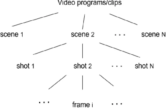
The general structure of a digital video is depicted in Figure 1.1. A digital video sequence consists of a sequence of still images taken at a certain rate. A video clip may contain many frames. Fortunately, video is normally made of a number of logical units or segments, namely video shots. Video scenes, on the other hand may contain a number of contigious video shots. In this study, we define video scene having high level semantics that are extracted from video data and also referred to as concept.
Figure 1.1 General structure of a video segment 1.4 Challenges
Automatic annotation of images is a challenging task because of “semantic gap” phenomenon which is the difference between understanding of visual concepts and image appearances. Overcoming semantic gap limitations is even harder in the presence of clutter, occlusion, camera shaking, viewpoint changes and various other noise sources inherent in images and videos [33]. Seperating a foreground
3
object from its integrated background is much like a chicken-egg paradox, where classification of one implies identification of the other and vice versa. This further restrict us to use algorithms from vision areas other than background segmentation. In addition to visual challenges, heavy nature of image and video data causes demanding solutions in this line of field. Algorithms should be reaching optimum classification and recognition accuracy while keeping memory and computation resource usage at a minimum so that vasts amount of multimedia data can be better processed. With the introduction of big data into the picture, we believe requirements force use of more elegant solutions. For instance, hours of video content is uploaded to cloud services each day and even real-time performing applications may be classified as infeasible solutions.
1.5 Thesis Statement and Claims
In this thesis we assume that semantic content of a video scene can be anything; for instance it can be a very coarse classification like indoor and outdoor scenes, or it can be the determination of various human actions present in the videos, even it may be recognition of object categories. This forces us to discover relationships between low-level image features and high level semantics of a scene from a given dataset. Hence, we avoid crafting hand-made relationships or using rule-based approaches for the sake of generalizability.
In addition to mentioned assumption of concept classification, with this thesis we
aim to show effectiveness of two state-of-the-art methods, namely the bag-of-words (BoW) based representations and deep learning for image and video
concept classification and image retrieval. We show efficient vector quantization (VQ) encoding practices along recent deep learning techniques.
1.6 Organization
Organization of this thesis is as follows; Chapter 2 presents related work on our field of research. Chapter 3 presents details of our BoW framework as well as obtained empirical results. In Chapter 4, we describe our deep learning method and present its applications to visual concept classification. In Chapter 5, we investigate content-based image retrieval as well as concept-based retrieval. We conclude in the Chapter 6.
4 1.7 Original Contributions
In this thesis, we introduce a very efficient BoW processing pipeline and show how to optimize each different step. We also show how convolutional neural networks (CNNs) can be combined with BoW paradigm to further push classification accuracy. We present state-of-the-art results on various benchmark datasets. Specifically, the contributions of this thesis are three folds:
We compare BoW and CNN architectures on common dataset and use identical processing pipelines.
We analyze the effects of parameter selection to the overall classification accuracy.
We also offer best practices for reaching state-of-the-art results on various benchmark datasets both in terms of computation efficiency and classification accuracy.
The work presented in this thesis has been published or submitted to following conferences:
Chapter 3 is published in Signal Processing and Communications Applications Conference in 2014.
Chapter 4 is submitted to The Second IEEE International Conference on Multimedia Big Data 2016.
Chapter 5 is published in Flexible Query Answering Systems Conference in 2015.
1.8 Software Libraries Used
Through out thesis study, we used various open-source libraries in our implementations. Our software packages use OpenCV [6] heavily, in many different places. We use Support Vector Machine (SVM) libraries provided by [7] and [18]. We use VLFeat both for feature mapping and extraction [73], as well Oxford VGG groups encoder evaluation software kit [8]. Our CNN implementations are using Caffe framework [26]. Last but not the least, we use Matlab more than often in our implementations [47].
5 2 LITERATURE REVIEW
2.1 Related Works on BoW Representation
Normally we would like to present a review of published studies under different sections for classification and retrieval as they are totally different problem domains. We still do this in the following sub-sections, however, we think it is more appropriate to start from common ancestors of both fields. Without such an introduction, we believe it is inevitable to loose some precise information about the history of these vision tasks. This is not only valid for classification and retrieval but also other fields of computer vision applications. For instance, both classification and retrieval algorithms find their early applications in texture recognition.
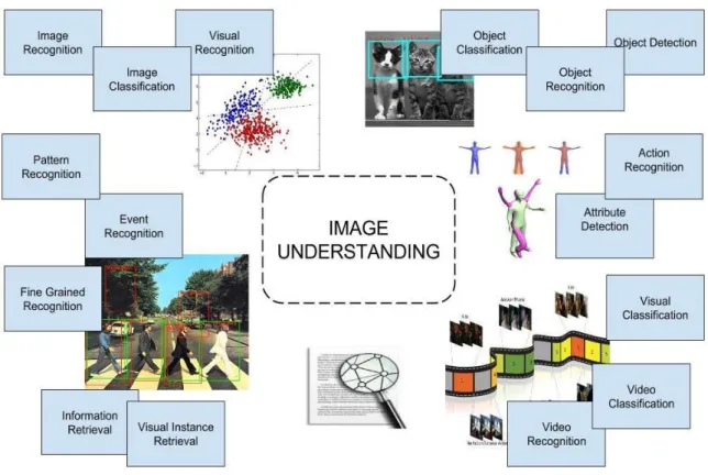
At this point we should emphasize that from a purely theoretical point of view, one can categorize vision applications into a wide selection of different topics with different requirements. There are many grifted categorizations present in the literature. Figure 2.1 shows results from our scan of existing literature and we believe this list is far from being complete. As it can be seen, many concepts are closely related to each other although solutions may be totally different. This grift relationship between different application areas forces us to treat these concepts as a single entity up to some point. We aggregate all these concept under the name of “Image understanding” wherever necessary throughout this study.
One of the very early object recognition approaches is to use direct pixel intensities or color at each pixel. This technique inherently assumes that images are cropped to region of interest and aligned in terms of pose and orientation which is not the case most of the time. Pixel intensity and color histograms can be viewed as global representations of an image [20]. Many object recognition studies employed parts-and-shapes models which uses spatial relationships between object components [85]. On the other hand, category wise object recognition or image classification enjoyed great success with the introduction of BoW paradigm which clearly become the choice of state-of-the-art methods in the literature.
6
Figure 2.1 Image understanding
In 2004, CSurka et. al. first proposed BoW for the visual categorization or image classification [10]. However, this was not the first application of BoW paradigm to the image understanding. In 1999, Leung et. al. applied [38] BoW to texture recognition. They create a vocabulary of outputs of a filter bank using k-means clustering. In their study, they ignore spatial information and use histogram representation of image textons. In a later study, Cula et. al. used BoW descriptors again for texture recognition. Like Leung, they create texton libraries by k-means clustering a set of image features. In 2002, Varma and Zisserman improved Leung with the addition of rotationally invariant filters [72]. In 2002, Zhu et. al. [87] applied it to image retrieval. They create a dictionary using generalized Lloyd’s algorithm which can be thought of a k-means variant. They use so called “keyblocks” of a given image instead of local image features. Naturally, their method is neither translation nor rotation invariant [10]. In 2003, Sivic et. al. applied BoW model to the video level object retrieval [63].
Following demonstration of success of BoW descriptors, many authors enhanced BoW representations for different image understanding tasks. Nister et. al. applied BoW representation to image retrieval from large selection of image dataset relatively using a higher number of dictionary dimension [49]. Laptev et. al. applied
7
BoW model to the video classification especially targeting human action categories [32]. Lazebnik et al. improved BoW classification by introducing spatial pyramids which incorporates lost spatial information into the BoW pipeline [33]. Yang et. al. replaced vector quantization step of BoW model with sparse coding and demonstrated state-of-the-art results on many image benchmark datasets [81]. In a similar study, Wang et. al. improved encoding performance of sparse coding using feature locality both in terms of performance and accuracy [76]. Van De Sande et. al. showed how color information can be inserted into BoW methodology [69]. Perronnin and Dance showed effectiveness of Fisher kernel (FK) encoding image category detection [51]. In order to improve quantization step of BoW, Philbin et al. introduced a method that uses soft assignment of image features to multiple visual codewords [54]. Gemert el. al. introduced a different way of soft assignment both addressing visual word plausibility and uncertainty [71] [70]. Jegou et al. introduced Hamming embedding for representing images with binary encodings [25].
2.2 Related Works on Deep Learning
In the recent years, CNNs have demonstrated excellent performance in plethora of computer vision applications. Most of this success is mainly attributed to two factors; recent availability of parallel processing architectures and larger image datasets [83] [62] [28]. Recent arrival of annotated and bigger sized datasets like ILSVRC [12], LabelMe [56] and MIT Places [86], made it possible to train deep convolutional networks for the task in hand without hitting the barrier of overfitting. Furthermore, accessibility of higher computational resources allowed researchers to design deeper networks with more parameters. For instance, top performer networks in ILSVRC challenge 2014 utilized more than 100 million parameters. Fusion of these two factors with better training algorithms [83] resulted in highly successful architectures performing state-of-the-art results in almost every field of computer vision.
One very important property of CNNs is their generalization ability. It is possible to apply a pre-trained network to a totally different dataset or application domain and achieve near state-of-the-art results. Moreover, with very little training effort they can beat most of other state-of-the-art approaches. This raises the question
8
whether they can be applied to application domains where diversity of data is a challenge. Recent studies indeed show that this is perfectly possible [55] [13]. CNNs adapted to various image understanding tasks including but not limited to image classification, object detection, localization, human pose estimation, event detection, action recognition, face detection, traffic sign recognition, street number recognition and handwritten digit classification. They have gained much attention in recent years, albeit they were introduced in the late 80s [36]. Krizhevsky et. al. applied CNNs to the task of image classification and demonstrated excellent results [31]. Zeiler showed how CNN models can be further developed using visualization techniques [83]. In the following years deeper architectures surfaced further pushing classification accuracies. Winners of classification and localization tasks of ILSVRC 2014 challenge [12] employed deeper architectures [65] [62]. Sermanet et. al. showed that CNNs can be trained to fulfill multiple image tasks like classification and localization together [58]. Latest studies reveal that much deeper architectures are expected to surface in the very near future [23].
Availability of massively parallel GPU architectures is enabling researchers for trying plethora of configuration options. One of the most common techniques is the fusion of different approaches. Wang et al. demonstrated how multiple CNN architectures trained on different datasets can be employed for increasing event recognition accuracy in images. Guo and Gould applied fusion of different networks to the object detection [22]. Chatfield et al. showed ensemble of CNN architectures with Fisher vectors, albeit their gain was marginal.
Application of CNN architectures to video domain is also extensive. Karpathy et al. showed how CNN models can be enriched with temporal information present in videos using several fusion techniques [30]. Simonyan et al. improved general approach to video action recognition using two stream convolutional networks [61]. Ye and friends further analyzed two stream architectures for video classification [82]. Wang et al. outlined good practices for action recognition in videos [78]. Zha et al. applied CNNs along with shallow architectures to video classification [84].
9
3 VIDEO CONCEPT CLASSIFICATION USING BoW REPRESENTATION 3.1 Methodology
3.1.1 Overview of Bag of Words
Bag of words (BoW) model is originally a document classification methodology later applied to image classification in early 2000s and up to recently it has been the mostly established image classification method in the literature due to its ability to fill semantic gap phenomenon to some extent. In its very basic form, BoW creates histograms of local image features counting occurrence of image features in the given image. It is an orderless representation of those features which discards spatial information. While loss of inherent spatial information of image content seems like inappropriate, this gives BoW representation some sort of invariance to image layout.
For creating histograms of local patches or features, BoW model employs a family of dictionary coding algorithms. Extracted local features of image are encoded to a more suitable representation in this coding step for later operations. Standing on this descripton, BoW based image classification can be best described in three different distinct phases; dictionary creation, training and testing. We need a suitable visual dictionary for training and testing phases. For visual dictionary creation, variations of well-known k-means clustering algorithms are mostly employed. A corpus is generated from training features and clustered into desired number of visual codewords. We investigate this process in more detail in section 3.1.2.
After visual dictionary creation phase, we train a classifier for the task in hand. We begin by extracting local features of training images. Later we encode extracted features using vector quantization (VQ) using visual dictionary. After this step, we count appearance of each codeword in the training image which becomes our BoW descriptor for the given image. As a final step, we train a suitable classifier using training data and corresponding labels. In the testing phase, we almost follow the same steps of training phase. We first extract local features and encode extracted features. After creating image histograms and BoW descriptors, we predict final category of the given image using the previously generated classifier. All of the mentioned phases are constituted of some common processing steps
10
which we name as the general BoW processing pipeline. This pipeline is composed of four operations; feature extraction, quantization, histogram generation and classification. These steps are visualized in Figure 3.1.
Figure 3.1 BoW pipeline
Several extensions exist to this paradigm in the literature. We investigate some of those extensions in the following sections but we need to mention some of them here for the sake of completeness. One of the possible extensions to classical BoW model is to use of spatial pyramids. In this approach, image is divided into smaller images and BoW model is independently applied to each smaller image. Later, these finer-grained image histograms are concatenated to create final image representation. Spatial pyramids provide a good cover for the spatial space and many state-of-the-art classification implementations use them directly or modified versions.
Some authors propose to overcome limitations VQ using better feature quantization techniques like sparse coding, Fisher encodings as well as employing soft assignment techniques instead of hard vector quantization. We further investigate various encoding schemes in section 3.1.4.
3.1.2 Visual dictionary creation
K-means clustering is by far the mostly employed technique for dictionary creation in the literature [75]. It is basically an unsupervised learning technique which finds desired number of cluster centers for a given data. It is an iterative algorithm, with each iteration new cluster centers are computed and each data point is assigned
11
to their closest center. While it is possible to use many distance metrics, Euclidean (or L2 distances) is the most obvious choice.
Let’s assume we’re given set of ”N” data points where each sample is “D” dimensional:
k-means aims to cluster these “N” data points into “K” clusters by minimizing the distance of each data point to their belonging cluster center:
After clustering operation, we export cluster centers for obtaining our so called visual dictionary composed of “K” visual codewords as modeled in Equation 3.3.
Minimizing objection function of Equation 3.2 is NP hard in practical use cases [45] which is overcome by using heuristic approaches like Lloyd’s algorithm [43] or Elkan’s algorithm [14]. One of the shortcomings of standard k-means algorithm is that it has run-time complexity of O(NK). Thus, it becomes hard to reach stabilization when dictionary size and number of samples increases. One alternative is to use hierarchical k-means clustering (HKM) introduced by [49] which has a complexity of O(NlogN) [75]. Another alternative is to use approximate k-means (AKM) algorithm of Philbin et. al. [53]. AKM has a run-time complexity of O(MNlogN) where “M” is the number nearest clusters accessed. Use of more advanced algorithms is not the only way for creation of more efficient dictionary generation. One other technique is to sub-sample input feature samples. This operation not only reduces both memory constraints and running times for clustering, it also helps to eliminate outliers in the input data.
Although k-means is the most widely used method of dictionary generation [80], there are several alternatives have been investigated in the literature. Jurie et. al. explored a mean-shift algorithm to overcome k-means favoring of most frequent
12
descriptors against rarely seen ones [29]. Some authors tried to come up with information theoretic semantic dictionaries using supervised learning methods [41] [34]. Tuytelaars et. al. divided feature space into regular grids instead clustering [67]. Wu et. al. [80] offered an alternative distance metric in place of Euclidean distance based on the histogram intersection kernel of Maji et. al [46]. Gaussian mixture models (GMMs) are also used to form dictionaries [50] [79].
3.1.3 Feature extraction
Feature extraction can be performed in two different approaches. One can use an interest point detector for detecting important points in image regions called keypoints. This scheme is called as sparse sampling as image features are extracted, relatively, from a set of sparse points. Various interest point detectors are present in the literature. Just to name a few we can say Laplacian of Gaussian, Difference of Gaussians, Harris detector, Hessian detector as well as their affine variant versions. Review of interest point detectors are beyond the scope of this study but additional information can be found in the literature [66] [57] [48]. Figure 3.2 visualizes a sparse sampling based feature detection.
Another alternative to interest point-based sampling is to dense sampling. In this scheme, features are extracted along a regular grid of points from the given image. Compared to sparse sampling, dense sampling produces much more image features. There is another alternative mentioned in the literature as random sampling where image features are extracted at randomly selected points from a given image. However, we believe this is only another form of dense sampling. Figure 3.3 visualizes a dense sampling based feature detection.
13
Figure 3.2 Feature extraction with Sparse Sampling
Many studies show the effectiveness of dense feature extraction over interest point based extraction on visual classification tasks [33], [27]. On the other hand, sparse sampling is employed in retrieval applications.
14 Scale-Invariant Feature descriptor
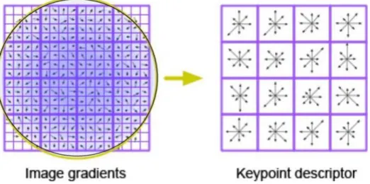
Our local image feature of choice is scale-invariant feature transform (SIFT) of [44]. SIFT is an image descriptor for image-based matching and recognition developed by David Lowe (1999, 2004). SIFT algorithm contains two distinct operations, keypoint detection and descriptor extraction. SIFT searches a given image for keypoints in a multi-scale fashion. Each detected keypoint has various attributes like position in scale space and orientation. SIFT is a said to detect ‘blobs’ in an image in contrast to edges. It uses Difference of Gaussian’s (DoG’s) image detector under the hood. SIFT descriptor, on the other hand, is a 3-D spatial histogram of the image gradients around a given keypoint, which is visualized in Figure 3.4. Due to its construction principles, SIFT image descriptor is invariant to translations, rotations and scaling transformations in the image space. It is also invariant, up to some degree, to moderate perspective transformations and illumination variations. Many studies in the literature shows the excellence of SIFT feature for image matching, object recognition and retrieval tasks.
Figure 3.4 SIFT feature descriptor representation 3.1.4 Feature encoding
Feature encoding is the process of re-coding local features to a more suitable notation for classification. Encoding doesn’t alter the local nature of the feature as it is pair-wise transform operation most of the time. There are many different encoding types present in the literature used with BoW. Hard vector quantization is one of the frequently used encodings which compares each feature with codewords in dictionary and assigns to the closest one. Soft assignment, improves this process by assigning to ‘k’ nearest neighbours instead of one. Sparse coding
15
is based on the relaxation of sparsity condition in vector quantization. Fisher vectors and super-vector encodings uses Gaussian Mixture Models and try to capture high-level relations of local features.
Now assuming we have our visual dictionary modeled by Equation 3.2, we extract our local image features in a dense fashion to obtain our image features:
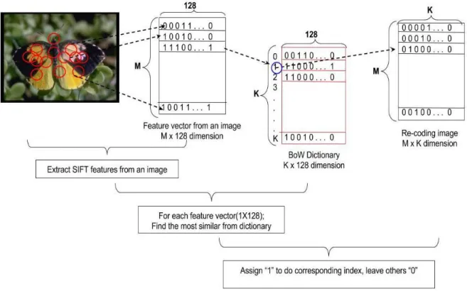
where each si is a “D” dimensional feature vector. We note that “D” is 128 for SIFT descriptors. Standard BoW model assigns every feature to the closest entry in our codebook, or dictionary:
Here d(.) represents a similarity measure and we use Euclidean distance to measure closeness of two vectors. This operation often is called a quantization operation since it discretizes a feature vectors. Equation 3.5 is also known as vector quantization and one of the most frequently used feature encodings, sometimes it is called hard assignment. Careful readers should notice that S’(𝜔) is an extremely sparse vector, i.e. only one entry of it is different than zero. 1/M term is present for normalization purposes, it cancels out the effect of different cardinalities of unevenly scaled images. Figure 3.5 visualizes this operation.
16
Figure 3.5 Vector coding visualization
Soft assignment is the process of quantizing local features in a soft manner, i.e. every feature contributes to more than one codeword in the dictionary. Soft assignment can modeled like:
According to Gemert et. al. [71], this type soft assignment deals with codeword uncertainty which indicates that one local feature may distribute probability mass to more than one codeword. With increasing size of dictionary size, soft assignment converges to hard assignment and soft assignment may help to improve accuracy for relatively small dictionary sizes. However, soft assignments gains can be marginal depending on the pipeline parameters and may not worth the waste of additional computational power. We call this type of coding scheme as KCB following the original author’s notation from now on.
Sparse coding is another alternative to vector quantization and poses some resemblance to soft assignment coding. It is based on the relaxation of sparsity condition in Equation 3.5. It encodes a local feature with a linear combination of a
17
sparse set of basis vectors [42]. Sparse coding can be represented as in Equation 3.7:
Wang et. al. [76] introduced feature space locality into sparse coding and further improved its computational efficiency. Their implementation is known as locality constrained linear coding, or LLC, in the literature. In addition to better representation of local image features, sparse coding encodings works well with linear classifiers which we mention about their importance more in detail in section 3.1.6. According to Yang et. al., this success can be mainly attributed to the much less quantization errors of sparse coding compared to vector quantization [81]. Fisher vector encoding uses Gaussian Mixture Model’s to learn higher order statistics of distributions of local features. Unlike BoW, it is not restricted by the occurrences of each visual word [52]. It can be tought of an extension of BoW as well as an soft encoding approach.
3.1.5 Spatial Pyramids
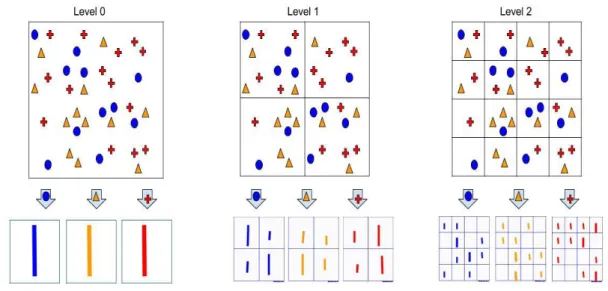
As we noted previously, BoW approach discards spatial layout of image features. Although this brings invariance to pose and geometric changes, to some degree, it also looses previous spatial information. Lazebnik et. al [33] introduced spatial pyramids method to take into account of rough scene geometry [52]. Spatial pyramids starts by dividing image into smaller grids which can either be regular or some irregular patterns. Then it calculates BoW descriptor for each sub-region of image. Grids can be created in multiple layers where going down the layers causing more fine-grained grid layouts. In the final representation, all histograms coming from all regions of all layers contribute to the final BoW descriptor, with some scheme of weight assignment taking in place. We re-depicted a well known visualization of spatial pyramids in Figure 3.6 where three different types of local features extracted from an image is shown. Level-0 refers to the whole image without any spatial partitioning. When we pass down to the Level-1, we create four different sub-regions of the image and calculate all corresponding histograms. We repeat same procedure with Level-2, but this time with a finer partitioning. Final image representation can be formed by concatenating all histograms into one
18
feature vector. We should emphasize that Level-0 representation belongs to the BoW representation without any spatial pyramid extension.
Figure 3.6 Spatial Pyramid visualization
One handicap of SPM extension is that it exploits feature dimensionality. Taking Level-2 into account, one ends up 21 (16 + 4 + 1) image regions. For Level-3, which is not depicted in Figure 3.6, this number rises to 85. Given that dictionary size is “K”, this results in final image feature size of 21 x K for Level-2. Although final descriptor size is bloated, SPM calculation is very efficient. Regardless of SPM level, nearest neighbours of each feature is searched only once due to the fact that location of a local feature in feature space is independent of its location in spatial space. With efficient programming practices, overhead of SPM generation is one of the fastest operations in whole processing pipeline.
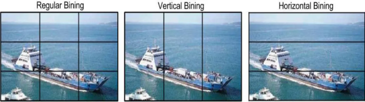
We should mention that SPM layout depicted is here taken from original authors’ [33] papers. Later studies also investigated different layouts like horizontal and vertical binning. For different datasets where object layouts differ significantly it may be more efficient to adapt such layouts. For instance, instead of dividing images into 16 square regions one may employ 3x1 horizontal binning or 4x1 vertical binning. Figure 3.7 visualizes different binning strategies.
19
Figure 3.7 Spatial Pyramid binning visualization 3.1.6 Classifier design
Machine learning is the art of learning structure from data and classifiers are the key components for linking data to its structure. In this regard, Support Vector Machines (SVMs) are among the most successful implementations. They were introduced in early 90s [5] [9] and gained much attention since then. They are designed as binary classifiers, several extensions exist for multi-class classification. SVMs are linear classifiers but they can be extended to non-linear cases by the use of a so called “kernel trick”.
Although non-linear SVMs are quite successful in many visual classification tasks, their performance comes at a high cost. Training of non-linear SVMs has a runtime complexity between O(N2) and O(N3) whereas linear SVMs have a complexity of
O(N), where “N” is the number of training images [60] [27] [81]. This makes use of non-linear SVMs impractical in case we have more than tens of thousands training data. On the other hand, linear SVMs are inferior to non-linear ones on many image processing tasks [52]. To overcome this drawback, many researchers seek for better encoders suitable for large-scale image and video classification tasks. Sparse coding and Fisher Vector encodings are just fruits of two of the many such research directions. We head towards a different route though. We choose to apply kernel mappings to our data prior to classification using homogeneous kernel maps [74]. These algorithms scale linearly with respect to training data while providing the same accuracy as the original non-linear SVM classifiers [52]. They are implemented for histogram intersection and X2 kernels which are the two most successful kernel types for our encoding operations [35] [59].
20 3.2 Datasets In Use
3.2.1 Caltech-101 dataset
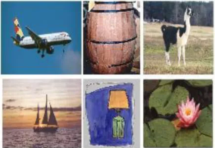
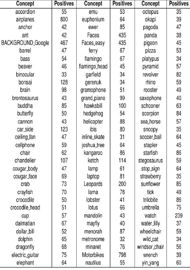
Caltech-101 dataset [19] contains 101 categories of different objects and one background which we use as a normal category in our experiments. Caltech-101 contains a total of 9,144 images and has 31 to 800 images per category. Moreover, most of the categories have more than 50 images. Average image resolution is around 300x200 pixels and each image contains only a single object. Caltech-101 is one of the most widely adapted datasets by computer vision community, for object recognition and classification tasks; as of this writing it has more than 800 citations in the literature making it one of the most important benchmark datasets for object recognition. Figure 3.8 shows some samples images taken from this dataset and summary of concepts present in the dataset is listed in Table 3.1.
Figure 3.8 Some examples from Caltech-101 dataset
Caltech-101 doesn’t provide any image lists for train and test case splitting. Common practice used in the literature is to randomly split dataset into two and then using one for training and the other one for testing. To prevent favorization effects of random splitting, results are reported on at least three different splits. Cross validation is not utilized at all. Most frequently used split regime is to use 30 train samples and rest for testing. Since results are presented using class-wise mean accuracy, un-even image sizes selected in testing phase is cancelled out.
21
Table 3.1 Summarization of concepts for Caltech-101 dataset
3.2.2 Caltech-256 dataset
Caltech-256 dataset [21] is an extension of Caltech-101 and it contains 256 object categories spanning total of 30607 images. Caltech-256 has the same structure as
22
Caltech-101 but with a better image distribution. When compared to Caltech-101, minimum number of images in any category is increased from 31 to 80. Like Caltech-101, Caltech-256 is also associated with object categorization and recognition and is cited by more than 1100 papers in the literature. Figure 3.9 shows some samples images taken from this dataset.
Figure 3.9 Some examples from Caltech-256 dataset
Validation procedure is much like Caltech101, only common choice for train split is to use 60 training images and rest for testing.
3.2.3 Pascal VOC 2007 dataset
The Pascal VOC 2007 [17] dataset is another benchmark dataset for image classification and localization. Pascal VOC 2007 contains 20 classes and a total of 9,963 images and 24,640 annotated objects. It is the predecessor of ILSVRC challenge. It has been cited more than 2800 papers in the literature. It is a harder dataset when compared to Caltech variations although has much less object classes. This is due to clutter and occulasion in the images as well as objects’ low spatial spanning in the training images. Another difference from Caltech datasets is that Pascal VOC supplies a training list so everyone uses same training and testing data for presenting their results. Pascal VOC also uses mean average-precision (mAP) measure instead of a simple accuracy measure used in Caltech datasets. Once again we present dataset structure in Table 3.2.
23
Table 3.2 Summarization of concepts for Pascal VOC 2007 dataset
3.3 Results
In this section, we investigate various aspects of BoW methodology. We start with effects of dictionary size on classification performance. We compare performance of different dictionary creation techniques on Caltech-101 dataset mentioned in section 3.1.2. We evaluate hierarchical clustering (HKM) with a corpus size of six-hundered thousands and three millions and normal k-means clustering with six-hundered thousands and we choose the most simple encoding scheme, vector coding without any extensions. However, we choose x2 SVM for best classification
accuracy. Our results are depicted in Figure 3.10 which uses a logarithmic scale to better represent diverse cluster range. We see that HKM yields almost same results with full k-means clustering which only has in edge over HKM for very small cluster sizes. With the increase of target dictionary sizes, HKM starts grasping the representation of corpus as well as full k-means. This tells us to favor HKM in place of full k-means in our classification pipelines. We once again emphasize that HKM has a run-time complexity of O(NlogN) and when compared to full k-means with complexity O(NK), it is a more suitable choice for large datasets.
Our second observation regarding Figure 3.10 is that increasing dictionary size effectively increases classification accuracy. This is especially true with higher dictionary sizes which can be marked as debatable deduction given the different observations present in the literature. For instance, Lazebnik et. al. shows that there is a limiting effect of increasing dictionary size beyond a certain limit [33]. This is in par with our previous studies presented in SIU 2014 [59]. We should
24
note that in both studies full k-means clustering is the choice dictionary generation algorithm. On the other hand, Chatfield et. al. [8] argues that increasing dictionary size always help to increase classification accuracy provided that feature encoding is not too lossy. We know that they use approximate k-means clustering (AKM) which is similar to HKM in terms of performance. These results suggests us to conclude that advanced clustering techniques like HKM and AKM are better at discriminating visual corpus compared to standard k-means algorithm even for big dictionary sizes. Given that they also have lower complexity than standard k-means algorithm they should be favored wherever possible.
Again [49] shows that using a larger corpus helps to cluster discriminatively better dictionaries when using large vocabularies. We observe same effect in our experiments. When using HKM clustering with more than three million feature corpus size, we observe higher classification accuracies than the previous six-hundered thousands case. Due to higher complexity of standard k-means algorithm, it is not feasible to increase corpus size for it above certain point. Given that HKM is both effective and discriminative with large a corpus, it is beneficial to increase corpus size up to a point where memory requirements is the limiting factor.
Next we investigate effects of different spatial pyramid level extensions on Caltech-101 dataset. We look into case of Spatial Pyramid (SPM) extension before investigating different feature encodings because SPM can be implemented regardless of the encoding choice. For SPM experiments we use VQ with HKM clustering for dictionary generation and same x2 SVM as in the previous dictionary
experiments. Figure 3.11 shows our results and Table 3.3 summarizes our numerical findings.
25
Figure 3.10 Classification accuracy with different dictionaries on Caltech-101 We observe that effects of SPMs is most dramatical with lower dictionary sizes. This implies that even if our visual dictionary is not discriminative enough to properly classify our dataset images, spatial information incorporated with SPMs adds up to classification accuracy. This adds some degree of robustness to our classification pipeline with respect to inadequate dictionary choices. Our second observation is that while using SPMs, increasing dictionary size beyond a certain limits results in almost no accuracy increase. For example taking two cases from Table 3.3, with L2 SPMs, 1000k dictionary size is only 1% worse than 5000k dictionary size.
Figure 3.11 Classification accuracy with different dictionaries and pyramid levels on Caltech-101
26
Table 3.3 Effects of SPM with different dictionaries sizes on Caltech-101
Next we investigate performances of different encoding types. This time we investigate feature encodings on more challenging Pascal VOC 2007 dataset. We fix dictionary size for all encodings as 4000k except for Fisher vector coding which we set-up to use 256 mixture models. For all encodings we fix feature extraction steps as pixel wide, both for horizontal and vertical resolutions. We extract SIFT features at multiple scales, also known as PHOW features [4]. We mix L1 spatial pyramids with three horizontal regions, totaling eight spatial regions. We use x2
SVM for VQ and KCB encodings since they are reported to be work better with those SVM types [8]. We also verified this in our SVM experiments. For FK and LLC encodings we use linear SVMs as those encodings get along with linear SVMs and don’t need non-linear kernels. For all our experiments, we select our SVM parameters either using grid search with 5-fold cross-validation in case of multiple parameters for non-linear SVM or using simple train-test validation for linear SVMs.
27
Table 3.4 lists our results. First thing striking us is the fact that VQ is reaching competitive results when compared to more advanced encodings, FK being the only exception. There are superior results for both LLC and KCB encodings when compared VQ encoding in the literature, however our results clearly states that this is not the case. Furthermore, there are other studies showing parallel results to our findings [8]. This can be attributed to various different phenomenon. First of all, unlike many studies, we follow a very aggressive feature extraction procedure. Both dense feature extraction step and images scales are used at limits. We believe this pushes performance of VQ further up whereas LLC and KCB is not taking advantage of denser feature extraction since they are already capable of coding image features at their optimum level. Another factor adding to this conclusion is that dictionary size can be increased further to make use of effectiveness of LLC and KCB encodings, as we believe they may further increase their performance with higher dictionary sizes. However, this increase is not be dramatic. For instance, [8] tested LLC with 25k dictionary sizes and they report 57.60% mAP on Pascal VOC 2007.
Our second observation is that none of these encodings are complementary. In Table 3.4 we listed winners and runners-up on a per-category basis. We see that FK encoding is the winner of all categories, and KCB is the runner-up in most of the categories. This makes us believe that success of any encoding is not dependant on any category, i.e. they get as discriminative as they can regardless of scene content. One other fact backing-up this theory is that categories with higher number of positive samples are always classified with higher accuracy. For instance, when we look into Table 3.2 we see that “Person” category has the highest number of positive samples and it is the category with highest AP in our results. This leads us to conclude that fusing different encodings types may not be a good candidate for multi-model image classification.
28
29
4 VIDEO CONCEPT CLASSIFICATION USING DEEP LEARNING 4.1 Methodology
4.1.1 Convolutional Neural Networks overview
Due to their recent success on many of the image processing tasks, we decide to import Convolutional Neural Networks (CNNs) into our processing pipelines. CNNs poses some unique properties for image understanding. First of all, they are highly
transferable, i.e. one network trained on a given dataset may achieve state-of-the-art results on other datasets provided that overfitting is overcome by a
suitable selection of training techniques. Secondly, they are highly parallel algorithms so vastly parallel architectures like graphical processing units (GPUs) can be utilized.
CNNs are biologically inspired feed-forward type artificial neural network architectures and they may be categorized as variants of multilayer perceptrons (MLP). Hubel and Wiesel [24] showed that biological visual cortex is composed of small cells sensitive to some part of visual field called receptive field. Receptive fields cover a portion of input image in a tiled arrangement of subregions which cover entire spatial correlations present in an image. There are two basic types revealed; simple cells responding maximally to edge like patterns in their receptive field and more complex cells, which have larger receptive fields, locally invariant to exact positions of input patterns. Early CNN architectures like LeNet [37] modelled this behaviour inherent in animal visual cortex. They found wide applications in image and video classification, natural language processing and many more computer vision tasks.
We investigate four different and popular CNN architectures in this part of our thesis. These CNN architectures are mostly winners or runners-up the famous image classification challenge ILSVRC [31] during their introduction time. CNN architectures are composed of a number of convolutional layers followed by subsampling layers. They may have additional fully-connected layers as well. CNN architectures all work with fixed input sizes but number of input color channels may vary from model to model. Given an image with resolution with size W x H and it is first resized to input resolution of the network, let’s say M x M. Assuming
30
we have an convolution layer at the input with kernel size “k”, stride “s” and padding “p”, this convolution layer produces “N” feature maps with size:
where “N” is fixed by network design. Each feature map then is subsampled using an average or max layers called pooling layers. After a stack of these multiple layers some fully-connected layers, which creates the vectoral outputs of a CNN, may follow. Figure 4.1 visualizes a generic CNN architecture layout.
Figure 4.1 CNN architecture visualization
Our first CNN architecture is AlexNet, first introduced by Krizhevsky et.al in 2012 [31]. AlexNet consists of eight layers, five of them being convolutional layers and three layers are being fully-connected layers. They have a last softmax layer which is not included in this layer list. Softmax layer is tuned for semantic classification of 1000 ImageNet, or ILSVRC, classes. In addition to softmax layer, there are various other max-pooling layers present in the architecture which is not counted in the layer list as well. In addition to those, there are hidden rectified linear units (RELU) following each of the convolution and fully-connected layers. This architecture is important in many ways, for instance it is the first demonstration of success of CNNs at such large scale. Moreover, it is not only successful in image classification tasks, for instance state-of-the-art results are reported for real-time pedesterian detection using a slightly modified version of AlexNet, recently [1].
31
We show details of AlexNet architecture in Table 4.1. All output dimensions are calculated by using Equation 4.1
Table 4.1 AlexNet network architecture
Our second CNN model of choice is the winner of 2014 ILSVRC challenge by Szegedy et, al. [65]. This network derives from a so called Network-in-Network architecture of Lin et. al. [39] and called GoogleNet. GoogleNet is deeper network than AlexNet, consisting of twenty-two layers if pooling layers are not counted. If all the independent blocks are counted, their architecture is said to have approximately 100 layers. Although being four times deeper than AlexNet, GoogleNet is only 2x times less-efficient during inference time compared to AlexNet. They reach this efficient while utilizing larger networks by the help of filter-level sparsity concept first stated by Arora et. al. [3]. Table 4.2 summarizes the general layout of GoogleNet. Please note that whole GoogleNet architecture has almost 100 layers which we don’t show all in detail in this table.
32
Table 4.2 GoogleNet network architecture
Our third and forth models are closely related to each other and introduced by Simonyan et. al. [62]. They secured second place of 2014 ILSVRC classification challenge, and won the same years localization challenge. They are code-named as VGG16 and VGG19 in the literature, latter being three layers deeper than the former. Their design is based on smaller convolutional filters in all layers of networks whereever possible. Smaller convolution steps permit them to increase network depth without too much increase in complexity. We show details of VGG networks in Table 4.3.
One of very important metrics for differentiating CNNs is their depth and number of parameters. Deeper networks with more parameters is harder to design and train, but often yield better results when compared shallower architectures. In Table 4.4 we provide various statistics about our CNN architectures.
33
Table 4.3 VGG19 network architecture
Table 4.4 Comparison of different network architectures
4.1.2 Classification strategies
We have various classification strategies using CNNs:
1. We can train a CNN end-to-end on our target datasets. 2. We can fine-tune pre-trained CNN on our target datasets.
34
3. We can use lower layers of CNNs as feature extractors and develop further encoding schemes.
4. We can use higher layers of CNNs and combine them with simpler classifiers like SVMs.
First item is not suitable for our case, mainly due to two reasons. One is training end-to-end networks requires high-end computational resources which we don’t have access through-out our thesis duration, secondly they require ultra-large scale datasets for achieving acceptable classification performance. For instance, GoogleNet was trained on a high-end distributed supercomputer of Google [11] and authors state that architecture can be trained on a few high-end GPUs in a week. VGG networks are not different than GoogleNet either in this regard, training one VGG network took three weeks using four top-notch GPUs in parallel [62].
Training CNNs end-to-end may cause severe overfitting if they are not trained with enough data. We extract some facts from literature [61] [30] to show ineffectiveness of end-to-end training on relatively small datasets and list those in Table 4.5.
Our second option of using CNNs for image classification is to fine-tune a pre-trained CNN for our datasets in hand. This is in fact an efficient way of performing classification as seem in Table 4.5, however, we don’t prefer this route as this step involves CNN training which is something we don’t have too much experience about.
Our third option is a new research are in the literature and we investigate this option in our thesis. In this type of classification, we extract feature maps from lower layers network architectures and treat them as local image features. Later we run our BoW pipeline on those feature maps. We present our findings in the results section with our personal comments.
Our forth option is to combine CNNs with simple classifiers, SVMs in our case. Unlike third method, we use upper layers of networks for feature extraction without any encoding taking in between feature extraction and SVM classification. This type classification is examined by various studies in the literature as well.
35
Table 4.5 End-to-end CNN training on UCF-101 video dataset
4.2 Datasets In Use
We report our findings on Caltech datasets which we mention on sections 3.2.1 and 3.2.2. In addition to Caltech datasets, we make use of UCF101 dataset [64]. UCF-101 is an action recognition dataset of realistic action videos, collected from YouTube. It consists of 101 action classes, over 13k clips and 27 hours of video data. UCF-101 currently the largest dataset of human actions. As most of the available action recognition datasets are not realistic and are staged by actors, UCF-101 aims to encourage further research into action recognition by learning and exploring new realistic action categories.
4.3 Results
We first investigate effects using lower layers of CNN architectures as local features and apply BoW methodology for image classification purposes. We choose AlexNet as our CNN model. For each of the CNN layers, we first extract local image features using feature maps of receptive fields in the CNN layers. Then we create a visual vocabulary. Later using this vocabulary, we encode local image features. As a final step, we apply level two spatial pyramids and map features using homogenous kernel mapping of type x2. We use linear classifiers
for classification, with cost parameter of SVMs set to 10.
Figure 4.2 summarizes our findings. By looking at the numbers we see that convolution layers should be choice for feature extraction as outputs of pooling and normalization layers perform worse significantly. Second of all, as we go deeper in the network layers, accuracy consistently increases. This can be attributed to learning ability of CNNs. In the very first layers, learned features are weak and less invariant to changes in the image structure. As we go deeper, with
36
the effects of more convolutions, learned features become stronger and with the effects of max-pooling layers they gain invariance to various imaging operations.
Figure 4.2 BoW methodology applied to CNN features on Caltech-101 Our most interesting finding is, though, features learned by network is almost better than hand-crafted features like SIFT for classification tasks. This leads to one another observation but we hold-on to that until we investigate other classification method of ours. In our second group of experiments, instead of extracting features from early layers and encoding them with BoW, we extract features from higher levels of our CNN architecture. We specifically choose final fully-connected layers for such a comparison. At a first glance, this is somehow expected to perform worse because we know that CNNs learn generic image features in the lower layers and more high-level semantics of images in the upper layers. Since our models are trained on an un-correlated and totally different dataset then we are using, we expect these semantics to be dataset specific. However, by looking our results shown in Table 4.6, we see this is not the case and CNNs achieve state-of-the-art results on our benchmark Caltech datasets. These unexpected results can be attributed to two distinct concepts. First, learned semantic features are more like mid-level image features rather than high-level image semantics. Secondly, CNNs are not only good at learning low-level image features, they are good at learning better encodings for those features as well. We must emphasize that CNN features perform equally well with linear SVMs.