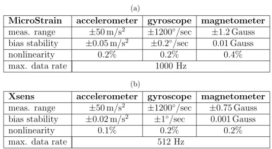
Deterministic and stochastic error modeling of inertial sensors and magnetometers
Tam metin
Şekil
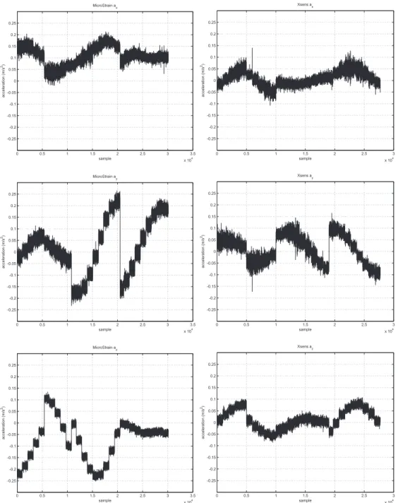
![Figure 1.1: Illustrations of the IMUs used in the thesis [1, 2]. (a) MicroStrain 3DM-GX2 and (b) Xsens MTx.](https://thumb-eu.123doks.com/thumbv2/9libnet/5669320.113484/16.918.197.773.252.488/figure-illustrations-imus-used-thesis-microstrain-xsens-mtx.webp)
![Figure 1.4: The JG7005 rate gyroscope used in 1950s [4].](https://thumb-eu.123doks.com/thumbv2/9libnet/5669320.113484/18.918.328.636.212.538/figure-jg-rate-gyroscope-used-s.webp)
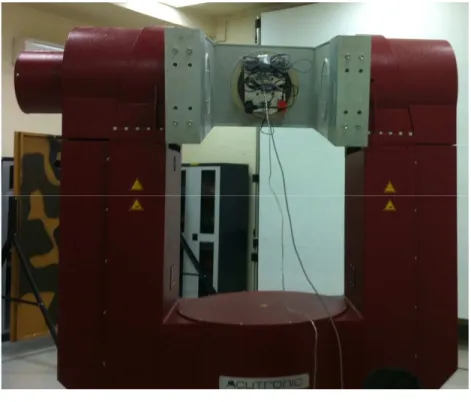
![Figure 1.5: An angular position control machine used for inertial sensor calibra- calibra-tion [5].](https://thumb-eu.123doks.com/thumbv2/9libnet/5669320.113484/21.918.315.651.443.772/figure-angular-position-control-machine-inertial-calibra-calibra.webp)
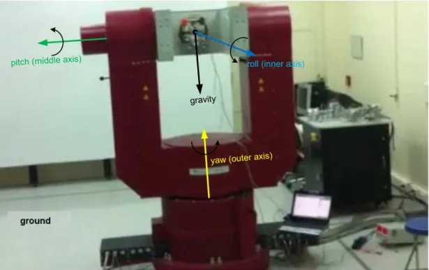
![Figure 2.3: Acutronic FMS overview (adopted from [9]).](https://thumb-eu.123doks.com/thumbv2/9libnet/5669320.113484/37.918.177.712.534.1020/figure-acutronic-fms-overview-adopted-from.webp)

Benzer Belgeler
Electrooxidation of methanol was realised on platinum and perchlorate anion doped polypyrrole film electrodes in acidic media.. A systematic kinetic investigation was performed
Bir kristaldeki düzenli ortam tarafından saçılan X-ı ş ınları, saçılmayı yapan merkezler arasındaki mesafe ı ş ın dalga boyu ile (X-ı ş ını dalga boyu)
Combining H1 –H3, we propose a moderated mediation model, shown in Figure 1, to test the relationship between followers ’ perceptions of leader Machiavellianism and quiescent
Fur- thermore, for a quadratic Gaussian signaling game problem, conditions for the existence of affine equilibrium policies as well as general informative equilibria are presented
Modifiye radikal mastektomi (MRM)’derı sonra seroma oluşumunu azalttığı düşünüldüğü için ameliyattan sonraki 7-10 gün arası hastanın ameliyat tarafındaki
Tedavi bitiminde FREMS ve TENS tedavisi grubundaki hastaların bel ve bacak ağrısı VAS, Oswestry Dizabilite Skoru, Roland-Morris Dizabilite Skoru, lateral fleksiyon ve el parmak-
değişikliği, hükümet darbele - ri gibi yüksek düzeyde toplum sal olaylar içindeki insanı ya - kalamaya çalışmak başlıca a- macı olmuştur.Bu nedenle r o
可抑制血管收縮素 II 所刺激的 HIF-1α 增加,血管收縮素 II 應是經由 PI3-K 路 徑而造成 HIF-1α 堆積,且 HIF-1α 表現與血管增生有關,因此血管收縮素 II 可能經
