Deep learning based cell segmentation in histopathological images

DEEP LEARNING BASED CELL

SEGMENTATION IN

HISTOPATHOLOGICAL IMAGES

a thesis submitted to

the graduate school of engineering and science

of bilkent university

in partial fulfillment of the requirements for

the degree of

master of science

in

computer engineering

By

Deniz Doğan

August 2018

DEEP LEARNING BASED CELL SEGMENTATION IN HISTOPATHOLOGICAL IMAGES

By Deniz Doğan August 2018

We certify that we have read this thesis and that in our opinion it is fully adequate, in scope and in quality, as a thesis for the degree of Master of Science.

Çiğdem Gündüz Demir(Advisor)

Hamdi Dibeklioğlu

Elif Sürer

Approved for the Graduate School of Engineering and Science:

Ezhan Karaşan

ABSTRACT

DEEP LEARNING BASED CELL SEGMENTATION IN

HISTOPATHOLOGICAL IMAGES

Deniz Doğan

M.S. in Computer Engineering Advisor: Çiğdem Gündüz Demir

August 2018

In digital pathology, cell imaging systems allow us to comprehend histopatholog-ical events at the cellular level. The first step in these systems is generally cell segmentation, which substantially affects the subsequent steps for an effective and reliable analysis of histopathological images. On the other hand, cell seg-mentation is a challenging task in histopathological images where there are cells with different pixel intensities and morphological characteristics. The approaches that integrate both pixel intensity and morphological characteristics of cells are likely to achieve successful segmentation results.

This thesis proposes a deep learning based approach for a reliable segmenta-tion of cells in the images of histopathological tissue samples stained with the routinely used hematoxylin and eosin technique. This approach introduces two stage convolutional neural networks that employ pixel intensities in the first stage and morphological cell features in the second stage. The proposed TwoStageCNN method is based on extracting cell features, related to cell morphology, from the class labels and posteriors generated in the first stage and uses the morpholog-ical cell features in the second stage for the final segmentation. We evaluate the proposed approach on 3428 cells and the experimental results show that our approach yields better segmentation results compared to different segmentation techniques.

Keywords: Deep learning, convolutional neural networks, cell segmentation, histopathological image analysis.

ÖZET

HİSTOPATOLOJİK GÖRÜNTÜLERDE DERİN

ÖĞRENME TABANLI HÜCRE BÖLÜTLEMESİ

Deniz Doğan

Bilgisayar Mühendisliği, Yüksek Lisans Tez Danışmanı: Çiğdem Gündüz Demir

Ağustos 2018

Dijital patolojide, hücre görüntüleme sistemleri, histopatolojik olayları hücresel düzeyde anlamamıza izin verir. Bu sistemlerde genellikle ilk adım, histopatolojik görüntülerin etkili ve güvenilir bir analizi için sonraki aşamaları büyük ölçüde etkileyen hücre bölütlemesidir. Diğer taraftan, hücre bölütlemesi, farklı piksel yoğunluklarına ve morfolojik özelliklere sahip hücrelerin bulunduğu histopatolojik görüntüler için zor bir iştir. Hücrelerin hem piksel yoğunluğunu hem de morfolojik özelliklerini bütünleştiren yaklaşımların, başarılı bölütleme sonuçlarına ulaşması muhtemeldir.

Bu tez, rutin olarak kullanılan hematoksilen ve eosin tekniği ile boyanmış histopatolojik doku örnek görüntülerinde hücrelerin güvenilir bölütlemesi için de-rin öğrenme tabanlı bir yaklaşım önermektedir. Bu yaklaşım, ilk aşamada piksel yoğunluğunu ve ikinci aşamada morfolojik hücre özniteliklerini kullananan iki aşamalı konvolüsyonel sinir ağlarını ortaya koymaktadır. Önerilen yöntem, hücre morfolojisi ile ilgili hücre özniteliklerinin, birinci aşamada üretilen sınıf etiket-lerinden ve olasılıklarından çıkarılmasına ve son bölütleme için ikinci aşamada morfolojik hücre özniteliklerinin kullanılmasına dayanmaktadır. Önerilen yak-laşım 3428 hücre üzerinde test edilmiş ve deneysel sonuçlar, yakyak-laşımımızın farklı bölütleme teknikleriyle karşılaştırıldığında daha iyi bölütleme sonuçları verdiğini göstermiştir.

Anahtar sözcükler : Derin öğrenme, konvolüsyonal sinir ağları, hücre bölütlemesi, histopatolojik görüntü analizi.

Acknowledgement

This thesis is the final step in my M.S. studies. I would like to thank all people who support and motivate me throughout this journey.

My first debt of gratitude undoubtedly goes to my supervisor Çiğdem Gündüz Demir for helping me finish this thesis. Without her support and guidance, I would not complete this thesis. Her door is always open to me whenever I encounter a difficult situation. I would also like to thank to Hamdi Dibeklioğlu and Elif Sürer for being in my jury committee and reviewing this thesis.

Annotating histopathological images is a challenging task that I could not handle by myself. Therefore, I specially thank to our medical experts Rengül Çetin Atalay and Ece Akhan for helping me in this task.

I owe my sincere thanks to my parents, Şengül Doğan and Kemal Doğan, and my sister, Duygu Doğan. Their love, support and sacrifice has always been a source of motivation for me.

Finally, my deepest gratitude is for my girlfriend, Çise Kanar. Her endless love and support encourage me in every way. There are no words to express my love to her.

Contents

2.1 Related Work on Cell Segmentation . . . 7

2.2 Deep Learning Background . . . 11

2.2.1 Convolutional Neural Networks . . . 12

3 Methodology 17

3.1 Stage 1: Intensity-Based Convolutional Neural Network . . . 19

3.2 Stage 2: Morphology-Based Convolutional Neural Network . . . . 26

3.2.1 Feature Extraction Layer . . . 26

CONTENTS vii

4 Experiments and Results 32

4.1 Dataset . . . 32

4.2 Parameter Selection . . . 35

4.3 Results and Comparisons . . . 36

5 Discussion 48

List of Figures

1.1 Sample HE stained liver tissue. . . 2

1.2 An example of a traditional cell segmentation procedure. (a) HE stained liver image. (b) Preprocessed image by stain deconvolution [1]. (c) Segmented cells after multilevel Otsu thresholding. (d) Postprocessed image by morphological operations. . . 3

1.3 An example of k-means based cell segmentation applied on two sample images. (a),(d) Sample images. (b),(e) Segmented cells. (c),(f) Precision results obtained on these images for different val-ues of k. Those two images exhibit their best precision results with different k values. . . . 4

2.1 Example of multilevel Otsu thresholding with three clusters. (a) Original image. (b) Result of multilevel Otsu thresholding. Blue pixels represent cell regions. (c) Binary cell image after applying small area removal, dilation, and hole filling operation, respectively. 9

2.2 Example of k-means clustering with three clusters. (a) Original image. (b) Result of k-means clustering applied on the RGB val-ues of pixels. Blue pixels represent cell regions. (c) Binary cell image after applying small area removal, dilation, and hole filling operation, respectively. . . 10

LIST OF FIGURES ix

2.3 Example of patch based CNN with two classes. (a) Original image and its gold standards. (b) Segmented cells after applying patch based CNN that classifies pixels as being cell or background. Note that each connected segmented cell is shown with a different color for the ease of visualization. . . 11

2.4 Sample autoencoder network. . . 13

2.5 Sample CNN architecture. . . 13

2.6 Padding operation for different pad sizes: (a) zero-padded matrix and (b) two-padded matrix. . . 14

2.7 Receptive fields for different dilation parameters: (a) dilation = 1, (b) dilation = 2, and (c) dilation = 3. . . . 15

2.8 ReLU activation function. . . 15

2.9 Sample MAX and AVERAGE pooling operations with 2 × 2 kernel and stride 2. (a) Sample 2-D matrix. (b) MAX pooling result. (c) AVERAGE pooling result. . . 16

3.1 Proposed TwoStageCNN model. . . . 18

3.2 Sample image patches for each class label. (a) Sample patches for the “background” class. (b) Sample patches for the “cell outer boundary” class. (c) Sample patches for the “cell center” class. (d) Sample patches for the “cell inner boundary” class. . . 20

3.3 (a) Original image. (b) Hematoxylin channel after applying the stain deconvolution. (c) Eosin channel after applying the stain deconvolution. (d) Residual channel after applying the stain de-convolution. . . 21

LIST OF FIGURES x

3.5 (a) Original subimage. (b) Its gold standard. (c) Annotated pix-els after applying the procedure given in Algorithm 1. Here blue, red, green, and white pixels represent “cell center”, “cell inner boundary”, “cell outer boundary”, and “background” classes, re-spectively. (d) Selected training pixels each of which is shown with a ‘+’ marker. A patch around each pixel is cropped and added to the training dataset. . . 25

3.6 (a) Sample subimage. (b) Gold standard. (c) Posterior map at the output of the first CNN classifier. (d) Posterior map at the output of the second CNN classifier. (e) Estimated class labels at the output of the first CNN classifier. (f) Estimated class labels at the output of the second CNN classifier. (g) Segmented cells after applying the region growing technique to labels in (e). (h) Segmented cells after applying the region growing technique to labels in (f). . . 31

4.1 (a)-(d) Subimages of normal hepatic tissues. (e)-(h) Subimages of hepatocellular carcinomatous tissues. . . 33

4.2 Visual comparisons of the proposed TwoStageCNN method with the ones using only one stage convolutional neural networks on example subimages. (a) Subimages and their gold standards. Seg-mented cells found by (b) TwoStageCNN method, (c) 1S2C_CNN method, (d) 1S3C_CNN method, and (e) 1S4C_CNN method. . 37

4.3 Visual comparisons of the proposed TwoStageCNN method with the ones using two stage neural networks on example subim-ages. (a) Subimages and their gold standards. Segmented cells found by (b) TwoStageCNN method, (c) 2S2C_CNN method, (d) 2S3C_CNN method, and (e) 2S4C_ANN method. . . . 38

LIST OF FIGURES xi

4.4 Visual comparisons of the proposed TwoStageCNN method with the ones using handcrafted features on example subimages. (a) Subimages and their gold standards. Segmented cells found by (b) TwoStageCNN method, (c) ThresholdingMethod, and (d) K-MeansMethod. . . . 39

5.1 Visual results of the cell segmentation methods obtained on exam-ple subimages. (a) Subimage and its gold standard. Segmented cells found by (b) TwoStageCNN method and (c) 2S2C_CNN method. . . 49

5.2 Visual results of the cell segmentation methods obtained on exam-ple subimages. (a) Subimage and its gold standard. Segmented cells found by (b) TwoStageCNN method and (c) 2S3C_CNN method. . . 49

5.3 Visual results of the cell segmentation methods obtained on exam-ple subimages. (a) Subimage and its gold standard. Segmented cells found by (b) TwoStageCNN method and (c) 1S4C_CNN method. . . 51

5.4 Visual results of the cell segmentation methods obtained on exam-ple subimages. (a) Subimage and its gold standard. Segmented cells found by (b) TwoStageCNN method and (c) 2S4C_ANN method. . . 51

5.5 Visual results of the cell segmentation methods obtained on ex-ample subimages. (a) Subimage and its gold standard. Seg-mented cells found by (b) TwoStageCNN method, (c) Threshold-ing method, and (d) K-means method. . . 52

List of Tables

3.1 Layers for the proposed CNN model. . . 21

3.2 Hyperparameters for the proposed CNN model. . . 24

4.1 Component-wise evaluation results of the proposed TwoStageCNN method against different segmentation algorithms. The results are obtained on (a) the training set and (b) the test set. . . 40

4.2 Component-wise evaluation results of the proposed TwoStageCNN method against different segmentation algorithms in terms of pre-cision, recall, and F-score metrics. The results are obtained on (a) the training set and (b) the test set. . . 41

4.3 Pixel-wise evaluation results of the proposed TwoStageCNN method against different segmentation algorithms in terms of pre-cision, recall, and F-score metrics. The results are obtained on (a) the training set and (b) the test set. Note that these results are calculated only considering the one-to-one matches. . . 42

Chapter 1

Introduction

Histopathological examination of tissue samples at the cellular level is important for diagnosis and grading of cancer. The first step of this examination process generally requires segmentation of each cell in the tissue since morphological characteristics of cells have a significant role in tumor analysis and cancer grading. Manual segmentation of these cells is not only time consuming for pathologists but it is also subjective and prone to errors. Thus, automated segmentation of cells is a need to alleviate these problems. However, automated cell segmentation in the context of digital pathology has various challenges, some of which include: poor staining across slides, variability in tissue samples, and scanning issues due to microscopy.

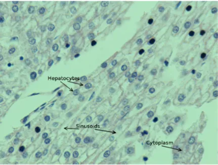
In this thesis, our goal is to segment cells1 in hematoxylin and eosin (HE) stained liver images. The HE technique is the staining process of tissue samples in which hematoxylin dye reacts with acidic components in the tissue and stains them with purplish color. Eosin dye reacts with basic components in the tissue and stains them with pink color. Hence, in HE stained images, nuclear regions are purplish since they contain acidic components and cytoplasm is pink since it is a basic component. A sample liver tissue structure is shown in Figure 1.1.

Figure 1.1: Sample HE stained liver tissue.

1.1

Motivation

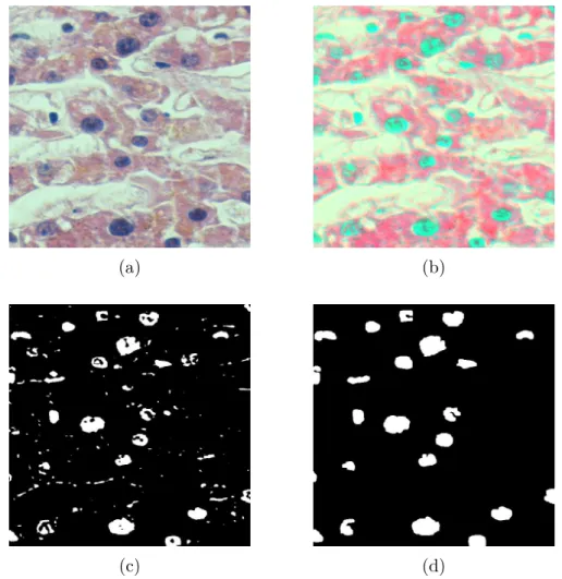
Traditional cell segmentation studies, which are based on handcrafted-features, usually follow similar steps. In their first steps, an image is preprocessed with image processing techniques (e.g., contrast enhancement, histogram equalization, and noise elimination) to improve the segmentation performance in the further stages. The second step constitutes the core method such that related image seg-mentation algorithms are run. The third one is the postprocessing step in which final improvements (e.g., small area elimination, morphological operations, and hole filling) are done. In Figure 1.2, an example of such a segmentation procedure is explained on a sample image. In this sample procedure, Otsu thresholding [3] is used as the core segmentation method.

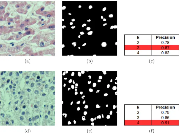
Although these traditional approaches, which use handcrafted-features, give promising results, they typically have the following problem. In most of these methods, there are too many parameters that require manual configuration and most of those parameters are image/tissue dependent. For example, Figure 1.3 shows the results of a cell segmentation procedure that includes k-means clus-tering followed by morphological operations. As seen in this figure, for the first

(a) (b)

(c) (d)

Figure 1.2: An example of a traditional cell segmentation procedure. (a) HE stained liver image. (b) Preprocessed image by stain deconvolution [1]. (c) Seg-mented cells after multilevel Otsu thresholding. (d) Postprocessed image by mor-phological operations.

image, the algorithm performs best in terms of the precision metric when k = 3 (see Figure 1.3 (a)-(c)). On the other hand, for the second image, the same algorithm performs best when k = 4 (see Figure 1.3 (d)-(f)).

In order to alleviate this problem, deep learning based approaches have been developed in recent years. In [4, 5], the studies do patch-based nucleus segmenta-tion using convolusegmenta-tional neural networks (CNNs). They first classify the extracted image patches as being positive or negative. Then, they segment the cells based on the posterior probabilities of image patches by finding regional maxima on the posterior map of the pixels. In a different study, multichannel deep learning

(a) (b) (c)

(d) (e) (f)

Figure 1.3: An example of k-means based cell segmentation applied on two sample images. (a),(d) Sample images. (b),(e) Segmented cells. (c),(f) Precision results obtained on these images for different values of k. Those two images exhibit their best precision results with different k values.

networks with two different deep learning models are used to generate posterior maps for both objects (cells) and edges (cell boundaries) [6]. Then, they integrate these posterior maps for the final segmentation. Hence, they also use boundary information of cells in order to improve the segmentation performance, especially on the cell boundaries.

These deep learning based approaches [4–6] automate the cell segmentation process without having to configure too many external parameters. However, most of these approaches use only intensity information of pixels and classify the patches as positive or negative. On the other hand, using other features together with the intensity may bring about additional information that can improve the segmentation performance. In response to this issue, this thesis proposes to de-sign a two-stage CNN that makes use of morphological characteristics of cells

in addition to the intensity information. To this end, it proposes to pose the problem as a multiclass classification problem, in which additional classes be-sides foreground and background are defined, and introduces an algorithm that effectively processes this extra class information to define and extract meaningful morphological features, which prove useful in accurate cell segmentation.

1.2

Contribution

In this thesis, we propose a two-stage deep learning model, which we call TwoStageCNN, that allows us to incorporate both intensity and morphological characteristics of cells. Traditional CNNs perform cell segmentation by classifying image patches based on their intensity levels. Although this approach successfully models the differences in between foreground and background pixels, it does not make use of morphological properties of cells. However, this property is impor-tant since there usually exists intensity-level noise in histopathological images due to poor staining and scanning issues in microscopy. Some postprocessing meth-ods can be applied to eliminate intensity-level noise but these methmeth-ods usually depend on the selected parameters. In our model, we address this problem by automating this process by adding another stage to the learning algorithm which extracts and uses morphological features of cells.

The contributions of this thesis are three-fold:

• As opposed to the previous deep learning based models, which use a single-stage CNN, this thesis proposes to design and use two-single-stage cascaded CNNs. The first stage uses intensity values to classify the pixels. The second stage uses area and boundary based morphological features of cells, that are pro-posed to be extracted from posteriors outputted by the first stage CNN. • As its second contribution, in order to extract more efficient features, this

thesis proposes to group pixels into four classes unlike the previous methods, which mostly group their pixels into two classes. In addition to background

and cell classes, this thesis defines “cell inner boundary” and “cell outer boundary” classes that may encode extra information about the cell. This allows us to more efficiently encode the boundary information, and hence, to define and extract more useful morphological features to be used in the second stage. Without having these extra classes, it would not be possible to define some of these morphological features.

• This thesis uses deep learning for the purpose of automated cell segmenta-tion. It is one of the successful demonstrations that use deep learning in the context of cell segmentation for HE stained tissue images.

1.3

Outline

The outline of the remaining of this thesis is as follows: In Chapter 2, we re-view the cell segmentation studies in the literature and give background informa-tion about deep learning and convoluinforma-tional neural networks. In Chapter 3, we give the details of the proposed TwoStageCNN method that includes two-stage convolutional neural networks for cell segmentation in histopathological images. In Chapter 4, we present the experimental results and our parameter analysis. In Chapter 5, we discuss our experimental results and compare our proposed TwoStageCNN method with its counterparts. Finally, in Chapter 6, we conclude this thesis and discuss the future work.

Chapter 2

Background

Histopathological image analysis literature has focused on three main problems: classification, segmentation, and detection. In histopathology, the classification problem is described as assigning predefined labels to input images from different categories. Its examples include cancer grading, lesion classification, nuclei clas-sification (nuclei vs. nuclei), and blood vessel clasclas-sification (vessels vs. non-vessels) [7–11]. The segmentation problem refers to extracting meaningful regions of interest (ROIs) (e.g., nuclei, cytoplasm, glands, and epitelium) [5, 6, 12–24]. The detection problem is to find the locations of the ROIs in the image with-out delineating their exact boundaries (e.g., nuclei detection and mitosis detec-tion) [16, 25–27]. The remaining of this chapter gives a summary of the previous studies in the area of cell segmentation.

2.1

Related Work on Cell Segmentation

In the literature of automated cell segmentation, studies using handcrafted fea-tures generally follow a similar procedure. The first step of these studies is the separation of foreground and background pixels by using a binarization technique (e.g., thresholding and clustering). After binarization, isolated cells can directly

be located by finding the connected components at the output of that binary image. However, when the cells are not isolated, those overlapping cells should be splitted with some post processing techniques (e.g, marker-controlled water-sheds [28–32], Gaussian mixture models [15], and concave point detection [12,33]) in the further stages.

Thresholding is one of simplest techniques that is used for image binarization in which foreground and background pixels are separated based on their inten-sity levels. This simple technique is also widely used in histopathological images which exhibit different characteristics in foreground and background pixel inten-sity levels [34–42]. One of the most well-known thresholding methods is Otsu thresholding, which aims to find a threshold value that minimizes the weighted sum of within-class variances of background and foreground pixels [3]. It is also employed in cell segmentation studies [34–38]. This effective method can be ap-plied to a single channel grayscale image [34–36]. Alternatively, it can be apap-plied to each channel of an RGB image [37, 38] and the output of each channel is com-bined to obtain the binary image. An example of Otsu thresholding is illustrated in Figure 2.1.

Otsu thresholding is good at extracting foreground pixels (cells) from back-ground in histopathological images. However, non-uniform illumination in the image is a problem for Otsu thresholding. This technique assumes that image has uniform illumination. In order to deal with changing illumination conditions in the histopathology images, different thresholding values are selected for differ-ent image regions by taking their local information into account [40–42], which is known as local adaptive thresholding.

Clustering is another technique to obtain the binary map of an image. It groups the pixels in such a way that the distance within-cluster pixels are mini-mized and the distance between-cluster pixels are maximini-mized. Since foreground and background pixels show different characteristics in histopathological images, clustering-based methods are also employed in cell segmentation studies [43–47]. Different features can be used as an input to the clustering algorithm depending

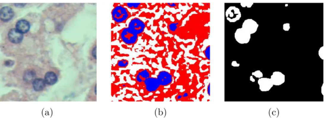
(a) (b) (c)

Figure 2.1: Example of multilevel Otsu thresholding with three clusters. (a) Original image. (b) Result of multilevel Otsu thresholding. Blue pixels represent cell regions. (c) Binary cell image after applying small area removal, dilation, and hole filling operation, respectively.

on the cell and image properties. Some studies use only intensity values of pix-els [43, 44] and some others also integrate the spatial information of pixpix-els [45, 46] as a feature to the clustering algorithm. The main drawback of clustering methods is to determine the number of clusters beforehand. To overcome this problem, a study integrates genetic algorithm with k-means clustering to determine the optimal number of clusters [47]. Clustering based methods are successful at sepa-rating cells and background pixels. Figure 2.2 illustrates an example segmentation result after applying k-means clustering on an RGB image.

Thresholding and clustering methods are used to obtain a binary map of the image. On that binary image, isolated cells could be identified. However, addi-tional postprocessing techniques are required to split the overlapping cells. One of the mostly used techniques to split overlapping cells is marker-controlled water-shed segmentation in which image is considered as a topographic surface. Then, regional minima/maxima are defined as markers on the intensity [28] or the dis-tance map [29] of the image and region growing starts from those markers. When two different marker sources are met, the image is splitted into two different com-ponents from those points. The problem here is that intensity/distance map of the image may have spurious markers which led to oversegmentation.

Therefore, the studies generally define markers after applying h-minima trans-form to suppress undesired minima/maxima smaller than h value [29–31]. The

(a) (b) (c)

Figure 2.2: Example of k-means clustering with three clusters. (a) Original image. (b) Result of k-means clustering applied on the RGB values of pixels. Blue pixels represent cell regions. (c) Binary cell image after applying small area removal, dilation, and hole filling operation, respectively.

key point in this marker-controlled watershed segmentation is to identify the h value. Smaller h values may lead to oversegmentation while larger h values may fail to separate touching cells. Therefore, they select h value adaptively [30] or by solving an optimization function [31] and use the same h value for the entire image. However, since cells may exhibit different characteristics within the image, using the same h value for the entire image may fail to identify some markers. To overcome this problem, a study selects multiple h values iteratively [32].

The model-based segmentation is another approach to segment overlapping cells. This approach builds its model based on the morphological characteristics of cells. One group of this approach separates the overlapping cells based on their roundness by modeling the distance map of overlapping cells as mixture of Gaussians [15], or constructing physically deformable models [14]. Another group uses concavity information and splits the touching cells from the detected concave points [12, 33]. Those model-based approaches are prone to fail and may lead to undersegmentation when cells are highly overlapping.

In recent years, deep learning based approaches have been preferred over the methods that use handcrafted features. Basically deep learning based approaches output class posteriors and the label for each input pixel. In doing so, some studies use patch based classification [4, 5], and some approaches use end-to-end classifi-cation [6]. For example, one group of studies classifies the input pixels into two

(a) (b)

Figure 2.3: Example of patch based CNN with two classes. (a) Original image and its gold standards. (b) Segmented cells after applying patch based CNN that classifies pixels as being cell or background. Note that each connected segmented cell is shown with a different color for the ease of visualization.

classes as nuclei and background based on the intensities of the patches cropped around each pixel [4, 5]. However, using only two classes may lead to poor seg-mentation performance on the boundaries and fail to segment overlapping cells which can be shown in Figure 2.3. To address this problem, they construct an end-to-end fully convolutional neural network and generate class posteriors for both cells and their boundaries at the output [6]. They, then fuse those two pos-terior maps for the final segmentation. Most of the deep learning approaches use only intensity information for the classification of pixels. However, morphological cell features may provide extra information that helps improve the segmenta-tion results. In this work, we incorporate pixel intensities and morphological cell features in our deep learning approach.

2.2

Deep Learning Background

Deep learning is a subfield of machine learning which is based on extracting high level features in the data through multiple layers of nonlinear transformations. Hierarchical structure of deep learning models allows us to represent complex relationships among data. Automatic feature learning ability of deep learning methods has made them more powerful than the conventional handcrafted-based machine learning algorithms. Due to the development of GPU chips and increase

in dataset sizes, deep learning based approaches have become more popular in recent years.

Different deep learning techniques are available based on the problem ad-dressed. One of the most commonly used unsupervised deep learning approaches is an autoencoder. The autoencoder is a special type of neural network in which input and output data are of the same size. In other words, an autoencoder maps input values to output values such that the first half of the network constitutes the encoding stage and its second half constitutes the decoding stage, as shown in Figure 2.4.

Another popular technique is the use of recurrent neural networks (RNN) and long short-term memory units (LSTMs) which are useful for identifying patterns in a sequence. Unlike feedforwarded networks, they also use past input values as a feedback to estimate their outputs. In this context, they can be regarded as networks with memory. Each deep learning technique can be used to address a different type of problem. In the next section, we explain convolutional neural network (CNN) architecture which is a very powerful deep learning approach for image segmentation tasks.

2.2.1

Convolutional Neural Networks

Convolutional neural networks, which are very useful for image segmentation and classification tasks, have an architecture (see Figure 2.5) generally consisting of the following layers:

Convolutional Layer is the most fundamental building block of CNNs such

that most of the computational jobs are done in this layer. This layer takes N-dimensional data as an input and generates an activation map for this input data with a set of filters. Filter values are updated at each iteration during training and each filter generates one activation map at the output. The formula for a 2-D convolution operation is given in Equation 2.1. In our proposed method, we use N-dimensional input data. In this case, N different 2-D convolution operations

Figure 2.4: Sample autoencoder network.

Figure 2.5: Sample CNN architecture.

take place. f [x, y] ∗ g[x, y] = ∞ X k=−∞ ∞ X l=−∞ f [k, l].g[x − k, y − l] (2.1)

A convolutional layer has the following parameters:

• Number of kernels: It determines the number of filters.

• Padding: It determines how many zero values are added to the border of the input data. This parameter is useful for preserving input and output data sizes. Figure 2.6 demonstrates zero-padded and two-padded 2-D input data.

      x11 x12 x13 . . . x1n x21 x22 x23 . . . x2n .. . ... ... . .. ... xd1 xd2 xd3 . . . xdn       (a)                 0 0 0 0 0 . . . 0 0 0 0 0 0 0 0 . . . 0 0 0 0 0 x11 x12 x13 . . . x1n 0 0 0 0 x21 x22 x23 . . . x2n 0 0 0 0 ... ... ... . .. ... 0 0 0 0 xd1 xd2 xd3 . . . xdn 0 0 0 0 0 0 0 . . . 0 0 0 0 0 0 0 0 . . . 0 0 0                 (b)

Figure 2.6: Padding operation for different pad sizes: (a) zero-padded matrix and (b) two-padded matrix.

• Stride: It controls how many pixels the filter slides over the input data during convolution.

• Weight filler: It determines how the filter coefficients are initialized (e.g., Gaussian and Xavier).

• Dilation: It is used to upsample the filters by inserting zeros between non-zero filter entries. Dilated convolution is especially effective to get a more contextual information. Figure 2.7 shows the receptive fields for different dilation parameters.

Rectified Linear Units (ReLU) Layer applies the activation function

given in Equation 2.2 on its input data so that negative input values are set to 0. In this way, adding some sparsity to the model will reduce cost by preventing excessive negative activations, especially in CNN architectures with too many neuron connections. Hence, one of the most important reasons to use the ReLU layer is to accelerate training process and adding some nonlinearity to the model. Figure 2.8 illustrates the ReLU function.

(a) (b) (c)

Figure 2.7: Receptive fields for different dilation parameters: (a) dilation = 1, (b) dilation = 2, and (c) dilation = 3.

−10 −5 0 5 10 0 2 4 6 8 10 x f (x )

Figure 2.8: ReLU activation function.

Normalization Layer performs the local response normalization (LRN)

op-eration over each local input region based on the opop-eration given in Equation 2.3.

(1 + (α/n)X

i

x2_i)β (2.3)

where α is a scaling parameter, β is an exponent, and n is the size of each local region [2]. In this equation, sum is calculated for each local region. LRN is useful for suppressing the unbounded activations like ReLU. It increases the contrast in the activation map which makes higher activation values more distinct within its neighborhood.

(a) (b) (c)

Figure 2.9: Sample MAX and AVERAGE pooling operations with 2 × 2 kernel and stride 2. (a) Sample 2-D matrix. (b) MAX pooling result. (c) AVERAGE pooling result.

layer reduces the computational cost since it reduces the number of parameters in a CNN. In addition, this layer prevents overfitting since it reduces spatial in-formation. Commonly used pooling operations are MAX and AVERAGE pooling which are illustrated in Figure 2.9.

Fully Connected Layer is the stage where final computations and decisions

are performed. Each node in the fully connected layer produces a single output from the weighted combinations of previous layer outputs. Every node in the previous layer is connected to every node in the fully connected layer. In other words, the fully connected layer combines the high-level features learned in the convolutional and pooling layers. Computed values are processed through a non-linear activation function (e.g., softmax) to produce a probability value so that each output node at the fully connected layer represents a probability of a certain class that the input data belongs to.

Chapter 3

Methodology

In this chapter, we explain the details of our proposed TwoStageCNN model which is a two-stage cascaded deep learning model that allows us to make use of both intensity and morphological features of cells. In the first CNN stage, we classify each pixel based on the intensity values of its belonging subregion and generate a posterior map to further use it in the second stage. In the second stage, we first extract morphological features (e.g., area and boundary related features) by using the class posteriors generated by the first stage and obtain feature maps for each pixel. Then, we classify the pixels based on the feature maps using another CNN and obtain final class labels and posteriors. For the final segmentation of cells, we use a region growing technique on the final class labels. The proposed TwoStageCNN model is illustrated in Figure 3.1 and its details are given in the following sections.

Training Patch Extraction

Sample training subimage Annotated subimage

Extracted image patches

Cell Segmentation

Stage 1: Posterior map

Stage 2: Posterior map

Segmented Cells Figure 3.1: Proposed TwoStageCNN model.

3.1

Stage

1:

Intensity-Based

Convolutional

Neural Network

The first stage deep learning model learns the label of a pixel and its class poste-riors which are to be used in the second stage to extract morphological features. To this end, this stage constructs a CNN which generates posteriors for each pixel based on the intensity values of a local patch with size wsize× wsizecentered

around that pixel. Pixels are classified using overlapping sliding window approach such that a patch is slided over the whole image by covering each pixel and for each pixel, four probability values are generated at the output which represent four predefined classes: “background”, “cell center”, “cell inner boundary”, and “cell outer boundary”. The main motivation behind using four classes instead of just using foreground and background classes is to ensure that the proposed model learns the boundaries better, and hence, yields better segmentation results for the overlapping cells. In Figure 3.2, sample image patches for each class label are shown. As shown in this figure, if we defined just two classes as foreground and background, then sample image patches in Figures 3.2 (a) and 3.2 (b) would be in the same class. However, as shown in Figures 3.2 (a) and 3.2 (b), they have completely different visual characteristics. Additionally, by defining four classes, it is possible to extract more informative morphological features such as the inner and outer boundary percentages.

The aim of this stage is to estimate the class labels and posteriors when an unannotated image is given. For this estimation, this thesis constructs a CNN classifier that takes pixel intensities as an input and generates posteriors and class labels for each pixel at the output. As the pixel intensities, instead of directly using RGB values, the image is transformed into another color space by applying the stain deconvolution operation, which is specifically defined for hematoxylin-and-eosin staining to emphasize nuclear regions more [1]. After that, the mean of pixels in the training image patches is calculated and image patches are normalized by subtracting this mean from the pixels of each patch. The stain deconvolution operation is illustrated in Figure 3.3.

(a) (b)

(c) (d)

Figure 3.2: Sample image patches for each class label. (a) Sample patches for the “background” class. (b) Sample patches for the “cell outer boundary” class. (c) Sample patches for the “cell center” class. (d) Sample patches for the “cell inner boundary” class.

The architecture of the proposed CNN is illustrated in Figure 3.4 and its layers are listed in Table 3.1. The architecture of the proposed model is inspired by the AlexNet CIFAR-10 architecture [48], which is used for natural image classification. Different than this architecture, our proposed network uses dilated convolutions instead of normal convolutions to get a more contextual information. Hyperparameters for the proposed CNN model are reported in Table 3.2.

(a) (b)

(c) (d)

Figure 3.3: (a) Original image. (b) Hematoxylin channel after applying the stain deconvolution. (c) Eosin channel after applying the stain deconvolution. (d) Residual channel after applying the stain deconvolution.

Table 3.1: Layers for the proposed CNN model.

Layer Layer Type Number of Kernels Kernel Size Stride Activation

0 Input 3 wsize× wsize -

-1 Convolution 64 3×3 2 ReLU+Norm 2 MAX Pooling 64 2×2 2 -3 Convolution 32 3×3 1 ReLU+Norm 4 MAX Pooling 32 2×2 2 -5 Convolution 32 3×3 1 ReLU 6 MAX Pooling 32 2×2 2 -7 Fully Connected 4 - -

-Figure 3.4: Prop osed CNN arc hitecture visualized b y the Caffe framew ork [2].

This CNN is trained for randomly selected pixels. For this purpose, a patch centered around each of these pixels is cropped and labeled with one of the four classes based on the annotated gold standard image. To annotate the gold stan-dard image G, two binary maps, namely Emap and Dmap, are generated by eroding

and dilating the cells in the gold standard image G, respectively. Then, each pixel pj is assigned to a label A(pj) based on Equation 3.1.

A(pj) =                      CellCenter if pj ∈ Emap

CellInnerBoundary if pj ∈ E/ map and pj ∈ G

CellOuterBoundary if pj ∈ G and p/ j ∈ Dmap

Background otherwise

(3.1)

This labeling procedure is also described in Algorithm 1. Here it is worth noting that we use a structuring element with a different size to erode different cells. The size of this structuring element is selected with respect to the size of the cell since the cells may be of varying sizes. For the dilation, the structuring element’s size is selected with respect to the patch size. (See Section 4.2 for the details of the selection of the structuring elements’ sizes.) Annotated pixels of a sample subimage, which are obtained after this procedure, are shown in Figure 3.5 (c). Note that the selection of pixels for the training dataset is not fully random. An equal number of pixels are randomly selected for each class label. The selected pixels for a sample subimage are shown in Figure 3.5 (d).

Table 3.2: Hyperparameters for the proposed CNN model.

Parameter Value Base learning rate 0.001 Momentum 0.9 Weight decay 0.004 Learning rate policy Fixed Batch size 100 Maximum epoch 10 Solver mode GPU

Algorithm 1 AnnotateImage

Input: gold standard image G with each cell having a unique id, patch size wsize,

multiplier dconstant for a structuring element of dilation, multiplier econstant for a

structuring element of erosion

Output: new annotated image A 1: Emap = ∅, Dmap = ∅, A = ∅

2: dsize= wsize× dconstant

3: for each cell Ci ∈ G do

4: _{Λ ← CalculateArea(Ci})

5: esize= Λ × econstant

6: T1 ← erode(Ci, disk(esize))

7: T2 ← dilate(Ci, disk(dsize))

8: Emap = Emap∪ T1 9: Dmap = Dmap∪ T2 10: end for

11: for each pixel pj ∈ G do

12: if pj ∈ Emap then

13: A(p_{j) ← CellCenter} 14: else if pj ∈ G then

15: A(p_{j) ← CellInnerBoundary} 16: else if pj ∈ Dmap then

17: A(pj) ← CellOuterBoundary

18: else

19: A(p_{j) ← Background}

20: end if

(a) (b)

(c) (d)

Figure 3.5: (a) Original subimage. (b) Its gold standard. (c) Annotated pixels after applying the procedure given in Algorithm 1. Here blue, red, green, and white pixels represent “cell center”, “cell inner boundary”, “cell outer boundary”, and “background” classes, respectively. (d) Selected training pixels each of which is shown with a ‘+’ marker. A patch around each pixel is cropped and added to the training dataset.

3.2

Stage 2: Morphology-Based Convolutional

Neural Network

The second stage deep learning model takes the pixels’ labels and their posteriors generated at the output of the first stage CNN as an input and extracts a set of morphological features from this input. Then, it generates feature maps for an image and uses those extracted feature maps in the second CNN classifier. This second CNN is trained to learn the label of each pixel based on the values in the feature maps for the final classification of this pixel. For the final segmentation of cells, a region growing algorithm is run on the output of the second CNN.

For this purpose, this stage first constructs a feature extraction layer between two CNN models. This extraction layer first finds the connected components of the pixels labeled with the “cell center” class by the first CNN classifier. Then it calculates a set of features for each connected component. At the end, it assigns the features of each connected component to every pixel in this connected component. For the pixels not belonging to any component, these features are set to zero. The following section explains the details of the feature extraction layer.

3.2.1

Feature Extraction Layer

The purpose of this layer is to define and extract a set of morphological features and introduce them to our deep learning model in order to utilize morphological characteristics of cells besides the intensity based features. To this end, this layer identifies each connected “cell center” component from the output of Stage 1 and defines the following morphological features for that component: “area”, “average cell center class score”, “inner boundary score percentage”, and “outer boundary score percentage”. Then, these component-level features are assigned to each pixel based on its belonging component so that each pixel in the feature map has four values that represent four predefined features. The details of these

extracted features are given as follows:

3.2.1.1 Component-Level Features

Let L = {Lcenter, Linner, Louter, Lbackground} be the label map and P =

{Pcenter, Pinner, Pouter, Pbackground} be the posterior map of an image I. Then,

connected components C on Lcenter are found and the following features are

ex-tracted for each connected component Ci ∈ C

Area feature is calculated as the area Λiof each connected component Ci ∈ C,

which is given in Equation 3.2.

Λi ← CalculateArea(Ci) (3.2)

Average cell score feature is calculated as the sum of Pcenter values of all

pixels within Ci ∈ C divided by its area Λi, which is given in Equation 3.3.

Θi ←

P

pj∈CiPcenter(pj)

Λi

(3.3)

Inner boundary score percentage feature represents the percentage of

boundary pixels of Ci that are adjacent to a pixel labeled as Linner. This

per-centage is weighted such that adjacent pixels with higher Pinner values have more

contribution. Calculation of inner boundary score percentage feature is given in Algorithm 2.

Outer boundary score percentage feature represents the percentage of

boundary pixels of Ci ∪ Ci(inner) that are adjacent to a pixel labeled as Louter.

Here note that Ci(inner) denotes the connected components found on Linner that

are adjacent to Ci. This percentage is also weighted such that adjacent pixels

with higher Pouter values have more contribution. Calculation of outer boundary

Algorithm 2 CalculateInnerPercentage

Input: connected components C, inner boundary class labels Linner and inner

boundary posteriors Pinner

Output: inner boundary score percentage Γ of components C 1: Γ = ∅

2: for each cell Ci ∈ C do

3: _{B ← FindBoundaryPixels(Ci})

4: N ← FindAdjacentPixels(B, Linner)

5: for each pixel pj ∈ N do

6: Γ(Ci) = Γ(Ci) + Pinner(pj)

7: end for

8: Γ(Ci) = Γ(Ci) / size(N )

9: end for

Algorithm 3 CalculateOuterPercentage

Input: connected components C, inner boundary class labels Linner, outer

bound-ary class labels Louter and outer boundary posteriors Pouter

Output: outer boundary score percentage Ω of components C 1: for each cell Ci ∈ C do

2: C_i(inner_{) ← FindAdjacentInnerComponents(Ci}, Linner)

3: U = Ci ∪ Ci(inner)

4: _{B ← FindBoundaryPixels(U )} 5: _{N ← FindAdjacentPixels(B, Louter})

6: for each pixel pj ∈ N do

7: Ω(Ci) = Ω(Ci) + Pouter(pj)

8: end for

9: Ω(Ci) = Ω(Ci) / size(N )

10: end for

3.2.1.2 Pixel-Level Features

After having calculated the features for each connected component Ci on Lcenter,

those feature values are assigned to each pixel based on the component Ci that

it belongs to and feature maps are generated for an image I. Each pixel pj in I

has four feature values F (pj) = {Farea(pj), Fscore(pj), Finnerperc(pj), Fouterperc(pj)}

representing four of the predefined features. The feature assignments at the pixel-level are given in Equations 3.4 – 3.7.

Farea(pj) =      Λ(Ci) if pj ∈ Ci 0 if pj ∈ C/ i ∀ i = 1...N (3.4) Fscore(pj) =      Θ(Ci) if pj ∈ Ci 0 if pj ∈ C/ i ∀ i = 1...N (3.5) Finnerperc(pj) =      Γ(Ci) if pj ∈ Ci 0 if pj ∈ C/ i ∀ i = 1...N (3.6) Fouterperc(pj) =      Ω(Ci) if pj ∈ Ci 0 if pj ∈ C/ i ∀ i = 1...N (3.7)

Then these four feature maps are combined to extract a four dimensional feature map F for a given image I.

3.2.2

Second Stage CNN Classifier

This CNN classifier aims to estimate the class label of each pixel for its final classification. It classifies the pixels based on the feature map F in order to utilize the morphological characteristics of the cells of an image I. For this purpose, it constructs a CNN classifier that takes pixel values of F as an input and generates class labels L2 and posterior maps P2. For a particular pixel, the input are the F values belonging to the local patch, with size wsize × wsize, centered around

this particular pixel. For each pixel, four probability values are generated by the second CNN, which again represent four of the predefined classes: “background”, “cell center”, “cell inner boundary”, and “cell outer boundary”. Note that by having this second CNN classifier, we aim to improve the class estimation.

This second CNN is also trained for randomly selected pixels. In order to be consistent with the first stage, same training pixels are used. To this end, a patch

is cropped in F centered around each of the selected pixels and labeled with one of the four classes based on Algorithm 1. Then, these patches are given as an input to train the second CNN classifier. The architecture and the hyperparameters of this CNN is the same with the first CNN classifier (see Table 3.1 and Table 3.2) except that the input data F is a 4-D tensor. After training the classifier, the class label and posteriors for each pixel are generated at the output. Then, this output is used in a region growing algorithm for the final cell segmentation.

This region growing technique is used for delineating cells on the final puted class labels of the second CNN. In this technique, each connected com-ponent, which is labeled as “cell center”, is grown on the pixels labeled as “cell inner boundary” until this component touches another grown connected com-ponent. This region growing algorithm is run at most N iterations. In each iteration, components are grown by one pixel towards each direction (i.e., right, left, top, and bottom). In this way, the boundary of the touching cells are better identified. In Figure 3.6, class posteriors, labels, and the segmented cells of a sample subimage are shown after applying the TwoStageCNN method and the region growing technique. Here note that if this region growing was applied on the posterior maps generated by the first CNN, the three components marked with arrows would not be splitted (see Figure 3.6 (g)). By using the second CNN, these maps are improved for better segmentation.

(a) (b)

(c) (d)

(e) (f)

(g) (h)

Figure 3.6: (a) Sample subimage. (b) Gold standard. (c) Posterior map at the output of the first CNN classifier. (d) Posterior map at the output of the second CNN classifier. (e) Estimated class labels at the output of the first CNN classifier. (f) Estimated class labels at the output of the second CNN classifier. (g) Segmented cells after applying the region growing technique to labels in (e). (h) Segmented cells after applying the region growing technique to labels in (f).

Chapter 4

Experiments and Results

4.1

Dataset

We conduct our experiments on 3428 cells taken from 20 different histopatho-logical tissue images which include both overlapping cells and isolated cells with different visual characteristics, sizes, and shapes. The dataset contains both hepatocellular carcinomatous and normal hepatic tissue samples stained with the hematoxylin-and-eosin technique. Each tissue image has a resolution of 1280×960 pixels captured by a Nikon Coolscope Digital Microscope with 40× objective lens. Each cell is annotated manually by our biologists collaborators and gold standard for each image is generated. Figure 4.1 illustrates example subimages of normal and cancerous tissues.

The dataset is randomly divided into training and test sets. The training set consists of 8 images, 4 normal hepatic and 4 hepatocellular carcinomatous tissue images, and contains a total of 1417 cells. The test set consists of 12 images, 6 normal hepatic and 6 hepatocellular carcinomatous tissue images, and contains a total of 2011 cells. The cells in the training set are used for parameter estimation and testing is performed using those estimated parameters. The cells in the test set are not used for parameter estimation in order not to obtain optimistic results.

(a) (b)

(c) (d)

(e) (f)

(g) (h)

Figure 4.1: (a)-(d) Subimages of normal hepatic tissues. (e)-(h) Subimages of hepatocellular carcinomatous tissues.

We evaluate our results based on two different criteria: component-wise eval-uation and pixel-wise evaleval-uation. In component-wise evaleval-uation, we observe the matchings of segmented connected cell components with the cells in gold stan-dards. To do that, we define “one-to-one”, “oversegmentation”, “undersegmen-tation”, “false detection”, and “miss” matchings for component-wise evaluation. Then, for pixel-wise evaluation, we find “true positive”, “false positive”, and “false negative” pixels. Note that we obtain pixel-wise evaluation results only considering the pixels of one-to-one matched cells.

Component-wise evaluation uses the following matchings:

• A segmented cell (and a gold standard cell) is evaluated as one-to-one match if the segmented cell is matched with a single gold standard cell which is not matched with any other cell1_.

• A gold standard cell is evaluated as oversegmentation if more than one segmented cell are matched with this gold standard cell.

• A segmented cell is evaluated as undersegmentation if it is matched with more than one gold standard cell.

• A segmented cell is evaluated as false detection if it is not matched with any gold standard cell.

• A gold standard cell is evaluated as miss if none of the segmented cells are matched with this gold standard cell.

Pixel-wise evaluation computes the following matchings on each one-to-one

matched cells:

Let C be one-to-one matched cells and G be annotated cells.

• True positive (TP) pixels are calculated as the number of pixels p such that p ∈ C and p ∈ G.

1_{Note that if more than fifty percent of the cells are overlapping, the cells are considered to}

• False positive (FP) pixels are calculated as the number of pixels p such that p ∈ C and p /∈ G.

• False negative (FN) pixels are calculated as the number of pixels p such that p /∈ C and p ∈ G.

Component-wise evaluations tell us how much percentage of the segmented cell components are matched one-to-one with gold standard cells. On the other hand, pixel-wise evaluations tell us how well pixels of segmented cells and gold standard cells are overlapping for one-to-one matches. Both evaluation criteria are important to measure the performance of the cell segmentation. After having calculated the component-wise and pixel-wise evaluation matchings, we define the following evaluation metrics to measure the performance of our proposed method.

For component-wise evaluation:

precision = number of one-to-one matches

number of computed cells (4.1)

recall = number of one-to-one matches

number of gold standard cells (4.2) For pixel-wise evaluation:

precision = T P

T P + F P (4.3)

recall = T P

T P + F N (4.4)

For both evaluations, we calculate the F-score as follows. F score = 2 . precision . recall

precision + recall (4.5)

4.2

Parameter Selection

The proposed method has four different parameters. The first two are used in the image annotation stage. The third parameter is used in CNN stages and

the fourth one is used in the region growing algorithm. The first two param-eters are econstant and dconstant, which are the constant multipliers to determine

the size of the structuring elements for erosion and dilation operation, respec-tively. The second parameter is the patch size wsize, which is the window size of

the extracted image patches. The fourth parameter is the number of iterations N , which determines the maximum number of iterations in the region growing process.

In our experiments, we use all possible combinations of the following pa-rameter sets wsize = {16, 32, 48, 64, 96}, econstant = {0.001, 0.005, 0.01},

dconstant = {1/6, 1/3, 1/2}, and N = {1, 5, 10}. From all combinations of these

parameter sets, we select the one that gives the highest F-score on the training images. After this step, the best parameters are selected as wsize= 64, econstant =

0.005, dconstant= 1/3, and N = 5.

4.3

Results and Comparisons

This section presents the quantitative and visual results obtained by our pro-posed TwoStageCNN method and compares them with the results of different algorithms. Evaluation results are obtained for both training and test sets. In Figures 4.2 (b), 4.3 (b), and 4.4 (b), visual results for the proposed method are shown for sample subimages. Note that in these figures, each cell is shown with a different color to better distinguish overlapping cells. From these examples, it can be seen that the proposed algorithm can successfully segment the overlapping cells. In order to better observe that the proposed algorithm works successfully, quantitative results are also obtained for both component-wise and pixel-wise evaluations. These quantitative results are given in the first rows of Tables 4.1, 4.2, and 4.3.

(a) (b) (c) (d) (e)

Figure 4.2: Visual comparisons of the proposed TwoStageCNN method with the ones using only one stage convolutional neural networks on example subim-ages. (a) Subimages and their gold standards. Segmented cells found by (b) TwoStageCNN method, (c) 1S2C_CNN method, (d) 1S3C_CNN method, and (e) 1S4C_CNN method.

(a) (b) (c) (d) (e)

Figure 4.3: Visual comparisons of the proposed TwoStageCNN method with the ones using two stage neural networks on example subimages. (a) Subimages and their gold standards. Segmented cells found by (b) TwoStageCNN method, (c) 2S2C_CNN method, (d) 2S3C_CNN method, and (e) 2S4C_ANN method.

(a) (b) (c) (d)

Figure 4.4: Visual comparisons of the proposed TwoStageCNN method with the ones using handcrafted features on example subimages. (a) Subimages and their gold standards. Segmented cells found by (b) TwoStageCNN method, (c) ThresholdingMethod, and (d) K-MeansMethod.

Table 4.1: Component-wise evaluation results of the proposed TwoStageCNN method against different segmentation algorithms. The results are obtained on (a) the training set and (b) the test set.

Group Method One-to-One Over. Under. False Miss Proposed TwoStageCNN 1374 0 17 48 7 One Stage 1S2C_CNN 1087 0 149 147 1 1S3C_CNN 1200 0 98 77 9 1S4C_CNN 1218 0 93 72 2 Two Stage 2S2C_CNN 1115 0 140 69 1 2S3C_CNN 1393 1 8 83 5 2S4C_ANN 1222 5 41 78 98 Handcrafted ThresholdingMethod 1012 48 73 178 202 K-MeansMethod 1041 44 75 154 172 (a)

Group Method One-to-One Over. Under. False Miss Proposed TwoStageCNN 1798 31 46 255 83 One Stage 1S2C_CNN 1316 1 274 385 19 1S3C_CNN 1532 3 194 276 59 1S4C_CNN 1593 5 171 268 39 Two Stage 2S2C_CNN 1340 0 263 274 37 2S3C_CNN 1789 45 51 304 60 2S4C_ANN 1626 32 75 223 172 Handcrafted ThresholdingMethod 1396 55 189 626 134 K-MeansMethod 1423 46 184 449 137 (b)

Table 4.2: Component-wise evaluation results of the proposed TwoStageCNN method against different segmentation algorithms in terms of precision, recall, and F-score metrics. The results are obtained on (a) the training set and (b) the test set.

Group Method Precision Recall F-Score Proposed TwoStageCNN 94.96 96.97 95.95 One Stage 1S2C_CNN 78.60 76.71 77.64 1S3C_CNN 87.02 84.69 85.84 1S4C_CNN 87.94 85.96 86.94 Two Stage 2S2C_CNN 84.21 78.69 81.36 2S3C_CNN 93.62 98.31 95.90 2S4C_ANN 87.91 86.24 87.07 Handcrafted ThresholdingMethod 66.98 71.42 69.13 K-MeansMethod 70.29 73.47 71.84 (a)

Group Method Precision Recall F-Score Proposed TwoStageCNN 81.39 89.41 85.21 One Stage 1S2C_CNN 66.20 65.44 65.82 , 1S3C_CNN 74.88 76.18 75.52 1S4C_CNN 77.41 79.21 78.30 Two Stage 2S2C_CNN 71.05 66.63 68.77 2S3C_CNN 78.57 88.96 83.44 2S4C_ANN 77.95 80.86 79.38 Handcrafted ThresholdingMethod 57.59 69.42 62.95 K-MeansMethod 63.24 70.76 66.79 (b)

Table 4.3: Pixel-wise evaluation results of the proposed TwoStageCNN method against different segmentation algorithms in terms of precision, recall, and F-score metrics. The results are obtained on (a) the training set and (b) the test set. Note that these results are calculated only considering the one-to-one matches.

Group Method Precision Recall F-Score Proposed TwoStageCNN 88.42 95.06 91.62 One Stage 1S2C_CNN 96.48 82.85 89.15 1S3C_CNN 98.03 83.32 90.08 1S4C_CNN 97.39 84.15 90.28 Two Stage 2S2C_CNN 97.04 81.47 88.58 2S3C_CNN 94.49 88.58 91.44 2S4C_ANN 91.16 80.39 85.43 Handcrafted ThresholdingMethod 86.41 90.73 88.52 K-MeansMethod 85.38 91.74 88.45 (a)

Group Method Precision Recall F-Score Proposed TwoStageCNN 88.23 88.52 88.37 One Stage 1S2C_CNN 92.07 81.00 86.18 1S3C_CNN 95.35 80.53 87.31 1S4C_CNN 95.11 80.33 87.10 Two Stage 2S2C_CNN 92.22 80.25 85.82 2S3C_CNN 92.74 83.00 87.60 2S4C_ANN 87.96 78.42 82.91 Handcrafted ThresholdingMethod 83.68 90.88 87.13 K-MeansMethod 84.83 91.13 87.87 (b)

In this section, we compare our proposed TwoStageCNN method against three different groups of approaches in order to evaluate its effectiveness. Those meth-ods are compared with our algorithm in terms of both visually and quantitatively.

The first and the second groups include the variants of our method. We use these methods to understand the effectiveness of different steps of our algorithm. In the first group of approaches, we use single stage CNN models to observe the effect of our model using an additional stage, which is included to model the morphological cell characteristics. These methods use only the first stage CNN classifier and classify the pixels based on their intensity values. Then, they extract cell labels. This group includes three methods:

• 1S2C_CNN has one stage CNN classifier and uses two classes, which are cell and background. This method is similar to the previous study [4] where they use AlexNet architecture [48] for patch based cell segmentation. • 1S3C_CNN has one stage CNN classifier and uses three classes, which

are cell center, background, and inner boundary. Then, pixels labeled with cell center and inner boundary classes are considered as cell pixels and cell center components are grown on the pixels labeled with inner boundary to identify final segmented cells.

• 1S4C_CNN has one stage CNN classifier and uses four classes, which are cell center, background, inner boundary, and outer boundary. Similar with the 1S3C_CNN method, pixels labeled with cell center and inner boundary classes are considered as cell pixels and cell center components are grown on the pixels labeled with inner boundary to identify final segmented cells.

The visual results for the 1S2C_CNN, 1S3C_CNN, and 1S4C_CNN methods are shown in Figures 4.2 (c), 4.2 (d), and 4.2 (e) and its quantitative results are given in the second, third, and fourth rows of Tables 4.1, 4.2, and 4.3, respectively. We use all the methods in this group to understand the effect of additional stage in our model. Visual results and component-wise evaluation results show that using an additional second stage decreases the number of undersegmentations. This

may be attributed to the following reason: The features that are introduced and extracted in the second stage allow us to better define boundary characteristics of cells. Hence, overlapping cells could be splitted successfully. Pixel-wise evaluation results also reveal that adding a second stage to the model ensures to obtain better segmentation performance especially on the cell boundaries. This is due to the fact that using boundary related features in the second stage (i.e., inner boundary and outer boundary score percentages) eliminates false pixels at the boundaries and thereby providing better delineation on cell boundaries (see Figures 4.2 and 4.3).

In the second group of approaches, we use two stage models to observe the ef-fect of using a different numbers of classes and a different type of classifier. These methods classify pixels using the intensity values in the first stage and morpho-logical cell features in their second stage. This group includes three methods:

• 2S2C_CNN has two stage CNN classifiers and uses two classes in the first stage, which are cell and background. Since it uses only two classes in the first stage, only a subset of features can be defined as the input of the second stage CNN. These features are area and average cell score, which are calculated similar to our proposed method. However, inner boundary and outer boundary score percentages features cannot be calculated since this method does not have inner boundary and outer boundary classes. • 2S3C_CNN has two stage CNN classifiers and uses three classes in the

first stage, which are cell center, background, and inner boundary. In the second stage, it uses area, average cell score, and inner boundary score percentage features. Since it uses inner boundary classes in the first stage, inner boundary score percentage feature can be calculated in the second stage in addition to area and average class score features. At the end, pixels labeled with cell center and inner boundary classes are considered as cell pixels and cell center components are grown on the pixels labeled with inner boundary to identify final segmented cells.

• 2S4C_ANN has two stage ANN classifiers and uses four classes, which are cell center, background, inner boundary, and outer boundary in the