Effect of burst length on loss probability in OBS networks with void-filling scheduling

EFFECT OF BURST LENGTH ON LOSS

PROBABILITY IN OBS NETWORKS WITH

VOID-FILLING SCHEDULING

a thesis

submitted to the department of electrical and

electronics engineering

and the institute of engineering and science

of bilkent university

in partial fulfillment of the requirements

for the degree of

master of science

By

Ahmet Kerim Kam¸cı

September, 2006

I certify that I have read this thesis and that in my opinion it is fully adequate, in scope and in quality, as a thesis for the degree of Master of Science.

Assoc. Prof. Dr. Ezhan Kara¸san(Supervisor)

I certify that I have read this thesis and that in my opinion it is fully adequate, in scope and in quality, as a thesis for the degree of Master of Science.

Assoc. Prof. Dr. Nail Akar

I certify that I have read this thesis and that in my opinion it is fully adequate, in scope and in quality, as a thesis for the degree of Master of Science.

Asst. Prof. Dr. ˙Ibrahim K¨orpeo˘glu

Approved for the Institute of Engineering and Science:

Prof. Dr. Mehmet B. Baray

Director of the Institute Engineering and Science ii

ABSTRACT

EFFECT OF BURST LENGTH ON LOSS

PROBABILITY IN OBS NETWORKS WITH

VOID-FILLING SCHEDULING

Ahmet Kerim Kam¸cı

M.S. in Electrical and Electronics Engineering Supervisor: Assoc. Prof. Dr. Ezhan Kara¸san

September, 2006

Optical burst switching (OBS) is a new transport architecture for the next gener-ation optical internet infrastructure which is necessary for the increasing demand of high speed data traffic. Optical burst switching stands between optical packet switching, which is technologically difficult, and optical circuit switching, which is not capable of efficiently transporting bursty internet traffic. Apart from its promising features, optical burst switching suffers from high traffic blocking prob-abilities. Wavelength conversion coupled with fiber delay lines (FDL) provide one of the best means of contention resolution in optical burst switching networks. In this thesis, we examine the relation between burst loss probability and burst sizes for void filling scheduling algorithms. Simulations are performed for various values of the processing and switching times and for different values of wave-lengths per fiber and FDL granularity. The main contribution of this thesis is the analysis of the relationship between burst sizes and processing time and FDL induced voids. This in turn creates a better understanding of the burstification and contention resolution mechanisms in OBS networks. We show that voids gen-erated during scheduling are governed by the FDL granularity and the product of the per-hop processing delay and residual number of hops until the destination. We also show that differentiation between bursts with different sizes is achieved for different network parameters and a differentiation mechanism based on burst lengths is proposed for OBS networks.

Keywords: Optical burst switching, fiber delay line, wavelength conversion,

Qual-ity of service.

¨

OZET

BOS¸LUK-DOLDURMA C

¸ ˙IZELGELEMES˙I KULLANAN

OBS A ˘

GLARINDA C

¸ O ˘

GUS¸MA UZUNLU ˘

GUNUN

KAYIP OLASILI ˘

GINA ETK˙IS˙I

Ahmet Kerim Kam¸cı

Elektrik ve Elektronik M¨uhendisli˘gi, Y¨uksek Lisans Tez Y¨oneticisi: Do¸c. Dr. Ezhan Kara¸san

Eyl¨ul, 2006

Optik ¸co˘gu¸sma anahtarlaması, artan y¨uksek hızlı bilgi trafi˘gi talebi i¸cin gerekli olan yeni jenerasyon optik internet altyapısı i¸cin olan bir ta¸sıma mimarisidir. Optik ¸co˘gu¸sma anahtarlaması teknolojik olarak zor olan optik paket anahtarla-ması ile g¨un¨um¨uz¨un d¨uzensiz internet trafi˘gini verimli olarak ta¸sıyamayan op-tik devre anahtarlaması arasında yer alır. Umut verici ¨ozelliklerinin aksine, optik ¸co˘gu¸sma anahtarlamasının kar¸sıla¸stı˘gı en b¨uy¨uk g¨u¸cl¨uk, y¨uksek trafik tıkanıklı˘gı olasılı˘gıdır. Bo¸sluk kullanımından faydalanan dalga boyu d¨on¨u¸s¨um¨u ile optik lif gecikme hatlarının birlikte kullanımı optik ¸co˘gu¸sma anahtarlaması

a˘glarındaki en iyi ¸ceki¸sme ¸c¨oz¨umleme mekanizmalarından birini sa˘glar. Bu

tezde g¨oze ¸carpan ¸ceki¸sme ¸c¨oz¨umleme mekanizmaları ile optik ¸co˘gu¸sma boyutları arasındaki ba˘gıntılar incelenmi¸stir. Deneyler farklı, i¸sleme gecikmesi, anahtar-lama gecikmesi, dalga boyu sayısı, optik lif gecikme hatları sayısı ve ¨o˘ge boyutu i¸cin yapılmı¸stır. Bu tezin en b¨uy¨uk katkısı ¸co˘gu¸sma boyutları ile i¸sleme gecikmesi ve optik lif gecikme hatları nedenli bo¸slukların arasında ba˘glantının inceleniyor olu¸sudur. Bu ¸sekilde ¸co˘gu¸sma olu¸sturma ve ¸ceki¸sme ¸c¨oz¨umleme mekanizmaları hakkında daha iyi bir anlayı¸s yakaladık ve ¸cizelgeme sırasında olu¸san bo¸slukların optik lif gecikme hatları ve i¸sleme gecikmesi-hedef bo˘gum noktası uzaklı˘gı ¸carpımı ile idare edildi˘gini g¨osterdik. Ayrıca de˘gi¸sik a˘g parametreleri i¸cin de˘gi¸sik boyut-taki ¸co˘gu¸smalar arasında ayırım yapılabilece˘gini g¨ostererek, ¸co˘gu¸smalar arasında ¨oncelik farklılı˘gı sınıflandırması olu¸sturulabilece˘gini sergiledik.

Anahtar s¨ozc¨ukler : Optik ¸co˘gu¸sma anahtarlama, optik lif gecikme hattı,

dal-gaboyu de˘gi¸simi, hizmet niteli˘gi.

Acknowledgement

I would like to express my deep gratitude to my supervisor Assoc. Prof. Dr. Ezhan Kara¸san for his instructive comments and constant support throughout this study. I would like to express my special thanks to Assoc. Prof. Dr. Nail Akar and Asst. Prof. Dr. ˙Ibrahim K¨orpeo˘glu for showing keen interest to the subject matter and accepting to read and review the thesis.

I would also like to thank my friends Kaan Do˘gan, Onur Kele¸s and C¸ a˘grı

Latifo˘glu for many helpful suggestions and discussions.

Finally, I would like to thank Ceyda M. Polat for her constant moral support.

Contents

1 Introduction 1

2 Optical Burst Switching Networks 8

2.1 An Overview of OBS . . . 8

2.1.1 Burst Assembly Mechanism . . . 13

2.1.2 Reservation Schemes and Protocols . . . 16

2.2 Contention Resolution in Optical Burst Switching . . . 18

2.2.1 Contention Resolution Algorithms . . . 20

2.3 Quality of Service in OBS . . . 23

2.3.1 Service Differentiation during Assembly-Time . . . 24

2.3.2 Service Differentiation during Reservation . . . 24

2.3.3 Service Differentiation during Scheduling . . . 25

2.3.4 Service Differentiation during Contention Resolution . . . 26

3 Loss Analysis in OBS Networks 27 3.1 Void Characterization in OBS . . . 27

CONTENTS vii

3.2 OBS Simulator . . . 29

3.2.1 Network Topology and Simulation Parameters . . . 30

3.3 Numerical Results and Discussions . . . 33

3.3.1 Effects of FDL Parameters and Number of Wavelengths . . 33

3.3.2 Effects of Voids on loss Probabilities . . . 35

3.3.3 Switching Delay . . . 39

3.3.4 QoS in OBS . . . 41

4 Conclusions 47

List of Figures

1.1 Voids in the scheduling plane of a core node . . . 4

1.2 Generation of voids in OBS . . . 5

2.1 Optical switching paradigms . . . 9

2.2 Optical burst switching . . . 11

2.3 Optical burst switching . . . 12

2.4 Optical burst switching network . . . 14

2.5 Burst assembly architecture . . . 15

2.6 JET protocol . . . 17

2.7 An example of FDL modules . . . 19

2.8 First fit algorithm example . . . 20

2.9 Lauc algorithm example . . . 21

2.10 Lauc-VF algorithm example . . . 22

3.1 Burst arrivals, Basic outline of the simulated architecture . . . 30

3.2 Burst generation process . . . 31 viii

LIST OF FIGURES ix

3.3 Number of wavelengths vs average loss probability, ρ=40%,

NF DL=16, D=50µs, Tp=50µs, Ts=0µs . . . . 34

3.4 Total FDL delay vs burst length histogram, ρ=30%, Tp=20µs,

Ts=0µs . . . . 35

3.5 Total Fdl delay vs Overall Loss Probability, ρ=30%, Ts=0µs . . . 36

3.6 Loss Probability vs Burst Size for total FDL delay of 400us,

ρ=30%, Tp=20µs, Ts=0µs . . . . 37

3.7 Loss Probability vs Burst Size for total FDL delay of 100µs,

ρ=30%, Tp=20µs, Ts=0µs . . . . 38

3.8 Voids histogram for ρ=30%, Tp=20µs, Ts=0µs . . . . 39

3.9 Void histogram with no FDL used, ρ=30%, Tp=20µs, Ts=0µs . . 40

3.10 Flattening points of loss probability curves for various processing

delays, ρ=30%, NF DL=4, D=25µs, Ts=0µs . . . . 41

3.11 Burst loss probability for each destination, ρ= 30%, NF DL=4

D=25µs, Tp=20µs, Ts=0µs . . . . 42

3.12 Overall effect of switching delay . . . 43

3.13 Effects of switching delay on loss probabilities for various burst sizes 44 3.14 Ratio between the loss probability of the longest burst vs the

small-est burst, ρ=30%, Ts=1µs . . . . 45

Chapter 1

Introduction

The demand for higher bandwidth on the Internet has been rising over the past decade. With the emergence of HDTV video conferencing, 3G networks and de-crease in subscriber service prices, the demand for broadband services will even be higher in the upcoming years. Fiber optic cables which can transfer the data faster to longer distances with greater reliability then copper wires are the cur-rent solution for the high traffic demand. The usage of Wavelength Division Multiplexing (WDM) [1] in optical networks, substantially increases the trans-mission rates over the fiber optic cables. In WDM, several data sources are multiplexed into the same fiber using different frequencies (wavelengths). With WDM technology, data speeds up to 1.6 Tbits/s per fiber has been demonstrated [2]. Unfortunately, the electronics based equipment used in the Internet infras-tructure (optical-electrical-optical converters, electrical processing modules) may not be able to cope with this huge bandwidth and the electro-optic equipment are also costly. In order to fully utilize the accessible bandwidth, the necessity for electrical equipment must be minimized, paving the way for all-optical networks. Several optical realizations are proposed for WDM based optical networks. Among these paradigms, Optical Circuit Switching (OCS) can provide a steady bandwidth between two nodes with a high predetermined QoS, but lacks the ability to adapt to different traffic conditions and has low channel utilization. In OCS, an end-to-end all optical lightpath is set between two nodes creating a

CHAPTER 1. INTRODUCTION 2

seamless passage for data packets. But the two way reservation scheme over long distances in wide-area-networks, e.g., thousands of kilometers, introduces major delays and lower utilizations.

On the other hand, Optical Packet Switching (OPS) [3] provides a transpar-ent transfer for optical packets and work with the same principles as an electrical network. In OPS, packet header is processed optically or electronically at each intermediate node while the optical payload is delayed and then forwarded after the switch is configured. At present, fiber delay lines (FDL) are the practical so-lution to optical buffering, but they can only provide granular delays and FDLs are scarce and expensive resources. OPS seems to be the ideal method for band-width efficient optical switching, but lack of viable optical processing and storage technologies makes this paradigm infeasible as of today.

Finally, Optical Burst Switching (OBS) [4, 5] has the best of packet switch-ing and circuit switchswitch-ing in order to integrate bursty Internet traffic to optical networks. In OBS, the data coming from various applications that are destined for the same egress node are aggregated at each ingress node into optical packets, called bursts. Before the optical burst is transmitted, an out of band control packet containing the header information is sent into the network in order to make the necessary reservations. The control packet undergoes O/E/O conver-sions at each intermediate node and is processed electronically to configure the switch for the incoming burst. This reservation method is one way only so that the source node does not have to wait for a reply from the destination before transmitting a new burst and thus the bandwidth is used more efficiently. The offset-time between the transmission of the control packet and the optical burst, ensures that the switching configurations are completed at intermediate nodes before the arrival of the burst.

There are various protocols used for burst reservation in OBS networks. Amongst these mechanisms, in Tell-And-Go (TAG) [6, 7] the control packet re-serves the bandwidth along the path from source to destination while being tightly coupled with the data burst. In Just-In-Time (JIT) [8] the reservation is done as soon as the control packet is received at the intermediate node and stays reserved

CHAPTER 1. INTRODUCTION 3

until another explicit release packet is received. This process results in unused but otherwise available bandwidth throughout the network and causes lower uti-lization. Finally in Just-Enough-Time (JET) [9, 10] protocol the intermediate node’s resources are only reserved for the transfer duration of the data packet. The control packet includes the necessary information such as the offset-time and incoming burst’s length.

Amongst the proposed switching paradigms, OBS has the best of the two worlds with the ability to efficiently transfer especially bursty Internet traffic. Comparing with OCS, one way reservation protocols ensures that the data trans-fer can start without waiting for an acknowledgment from the destination node, thus harness the otherwise lost bandwidth resources. Using different channels for the control domain avoids the synchronization and buffering problems involved in OPS. However due to the one way reservation protocol and lack of optical memory, OBS suffers from high loss probabilities. Large loss probabilities can be reduced by using clever mechanisms so as to provide means for efficiently using the enormous bandwidth associated with optical transport. Contention in OBS occurs whenever two or more optical bursts try to leave the node at the same moment, from the same output port, using the same wavelength. For contention resolution, any of these variables may be altered. In wavelength domain, any of the contenting bursts may be sent to the next node over a different available wavelength by means of wavelength conversion. In the time domain, the burst can be delayed until the contending resources are once again available by means of fiber delay lines. Finally, using deflection routing, any of the contending bursts may be guided to another outgoing port to a different node, to be finally routed towards the destination node over a different path.

In this thesis, we focus on the contention resolution with wavelength conver-sion and fiber delay lines [5] in conjunction with the most widely used scheduling algorithm in OBS, namely Latest Available Unused Channel with Void Filling (Lauc-VF) [11] scheduling algorithm. The main advantage of Lauc-VF over other algorithms is it’s ability to utilize the otherwise lost bandwidth space called voids. Voids are unoccupied positions in the scheduling plane of a core node. Each

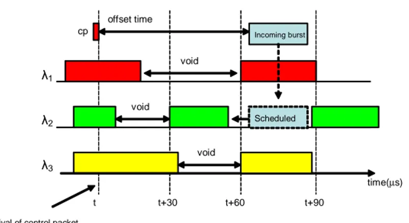
CHAPTER 1. INTRODUCTION 4 t+60 t t+30 λ1 λ2 λ3 Incoming burst offset time

Arrival of control packet

t+90 void void void time(µs) Scheduled cp

Figure 1.1: Voids in the scheduling plane of a core node

node in OBS has a table of currently scheduled bursts. This table is updated dynamically as the time passes. An example table can be seen in Figure 1.1. In the example, a control packet has just arrived at time t and is trying to schedule it’s associated burst after an offset time, at t+of f settime. Suppose at that time,

a vacant spot is available at wavelength λ2 and the burst is scheduled without

resorting to any contention resolution mechanism. In the scheduling plane, the time after no scheduling exists, is called the horizon of that channel. For instance

in Figure 1.1, the horizon time for wavelength λ1 and λ3 are both just before

t + 90. Horizon based algorithms such as LAUC [12], only keep track of these

horizon times for each wavelength and try to assign an incoming burst to the latest available horizon (as long as the horizon is earlier than the start time of the burst), so that the generated void size can be minimized. Horizon based algorithms are relatively simple and easy to implement. However these algorithms suffer from low utilization and high blocking probabilities, as they tend to discard all the generated voids.

Due to the nature of Horizon based algorithms, there is no distinction be-tween bursts with different sizes in terms of the loss probability, as all the bursts have to be traversed up to the horizon time of the output channel and only the burst starting time is important at that point. On the other hand, for void fill-ing schedulfill-ing algorithms, both the startfill-ing time and the length of the burst determine the successful transmission or loss of a given burst.

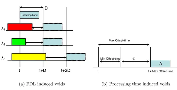
CHAPTER 1. INTRODUCTION 5 t+2D t t+D λ1 λ2 λ3 Incoming burst D

(a) FDL induced voids

t Max Offset-time Min Offset-time t + Max Offset-time A τ

(b) Processing time induced voids

Figure 1.2: Generation of voids in OBS

In order to fully appreciate the void filling mechanisms during scheduling, one must have the necessary information of void generation, when and how the voids are generated. We have two situations that generate voids during the scheduling phase in OBS. The first one is due to the usage of FDLs. This part can be best described with an example. In Figure 1.2(a), a burst arrives at time t. At the moment of its arrival, all the wavelengths are occupied. To prevent contention, depending on the scheduling algorithm in use, the node uses FDLs and might also use wavelength conversion. In the example, a trip in an FDL loop will induce a delay of Dµs. If a delay of D will not be enough to prevent contention, the burst can enter the FDL loop multiple times, to obtain a delay of BxDµs (where B varies from 1 to maximum number of FDLs available). The arriving burst can

be delayed for Dµs, so that it can be scheduled to λ1 or λ2. A delay of 2xDµs

is required if the scheduling is to be done to λ3. In all three cases the voids

generated by the use of FDLs and wavelength conversion will be varying such that 0µs < void size < Dµs. We call these voids FDL induced voids.

The second source for void generation in OBS is attributable to the offset-time differences between bursts in JET reservation mechanism. The one way reservation methodology in OBS, implies that all the reservations in a core node

CHAPTER 1. INTRODUCTION 6

will have to be made for future times. Unless the node is the destination of that specific burst, there will always be an offset time difference between the data burst and its control packet. This behavior inevitably generates voids. Lets see this in an example. In Figure 1.2(b) the offset-time induced void can be as long as the difference between the maximum offset time and the minimum offset time. Maximum offset time is calculated by the multiplication of maximum hops a burst must make in order to reach its destination by the processing time at each node. While the minimum offset time is used when the destination node is just one hop away and is equal to unit processing time. Lets say we are at time t and burst A’s control packet has just arrived and managed to get burst

A to be scheduled at (t − maxof f set). If a new control packet with minimum

available offset-time arrives just after t, it will have to face a void with size τ . τ denotes the maximum attainable void for the network and bursts bigger than τ will not be able to utilize voids. Depending on the offset-time differences of two consecutive control packets, the generated void’s size varies such as 0µs < void size < maxof f set − minof f set. We call voids generated in such manner, offset time induced voids.

The average size of void size and also their size distribution is of great im-portance for scheduling algorithms that utilize void filling, such as Lauc-VF. For instance if the average void size is smaller than most of the bursts in transit, the network will not be able to utilize those voids and the voids will most probably be wasted.

One trivial inference of void size and distribution knowledge is that, we can ar-range the burst sizes in such a manner that, only some of the bursts will be able to utilize the existing voids. Void generation mechanisms indicate that created voids are not affected by burst size choices unless a void is utilized during scheduling. This ensures that changing the burst size distribution will not greatly interfere with the generated void sizes and distribution. In the case of void utilization during scheduling, the burst is scheduled right into the void and will create two new voids, whose sizes depend on the burst size and the scheduling algorithm in use. For instance basic version of Lauc-VF, uses min-sv [13] approach where the scheduler tries to minimize the starting void, which stands for the void generated

CHAPTER 1. INTRODUCTION 7

between the starting time of the newly arriving void and the ending time of the previous burst in scheduling table.

Using the void size distributions, we can decide which bursts will be favored by void filling most (since they can fit into more voids) and which sizes will be handicapped as they will not be able to utilize voids. Simulation results indicate that, both the FDL induced and offset-time induced voids are able to create a class differentiation with different properties. FDL induced voids tend to cre-ate a more steep differentiation where only bursts smaller than FDL granularity is favored, while all other burst sizes have the same blocking probabilities. We managed to obtain burst loss probability ratios of up to more than 13 between burst sizes with the highest loss probability and with the lowest loss probability. On the other hand, offset time induced voids, tend to create a linear class dif-ferentiation between bursts of different sizes. Bursts larger than the maximum attainable void size will not be able to utilize voids at all and will all have same blocking probabilities. Using the offset induced voids, burst loss probability ra-tios exceeding 44 are obtained between the loss probabilities of the largest and smallest bursts.

The rest of the thesis is organized as follows: Literature search concerning Optical burst switching and related mechanisms such as reservation schemes and contention resolution mechanisms and quality of service are investigated in Chap-ter 2. ChapChap-ter 3 describes the simulation environment, the algorithms used and the parameters involved and presents the results obtained from simulations. Con-cluding remarks are presented in Chapter 4.

Chapter 2

Optical Burst Switching

Networks

In this chapter, some of the topics in optical burst switching networks pertaining to the thesis are presented. The chapter starts with a comparison of optical switching paradigms, continues with mechanisms and protocols governing OBS, such as burst assembly, reservation and scheduling protocols. The contention resolution mechanisms in OBS are then described and the chapter finally ends with currently proposed QoS mechanisms in OBS.

2.1

An Overview of OBS

Wavelength-division multiplexing (WDM) was first introduced in 1970 [1] and WDM systems were realized in laboratory in 1978 [14]. A WDM system uses a

multiplexer at the transmitter end to combine several optical signals at

differ-ent wavelengths and a demultiplexer at the receiving end to split the signals. Systems today can combine up to 160 10Gbit/s wavelengths together to achieve transmission of 1.6 Tbit/s over a single fiber. Currently WDM networks are used as major backbone links for long distance carriers who use synchronous optical network (SONET) as the standard interface. WDM is also quite popular for

CHAPTER 2. OPTICAL BURST SWITCHING NETWORKS 9 A B C D green blue red red

(a) Optical circuit switching

A B C D blue red green green blue

(b) Optical packet switching

Figure 2.1: Optical switching paradigms

telecommunications companies, as WDM allows the expansion of the network ca-pacity without the need of altering the physical layer, namely the optical fibers. The multiplexers and demultiplexers constituting the network can be upgraded seamlessly to increase the capacity.

One of the major problems with WDM is the necessity of very high speed electro-optical converters which alters optical data to electrical domain and vice versa to handle the large capacities of bandwidth provided. Even with the in-creasing electronic computing capabilities, electrical/optical and optical/electrical converters are having problem with coping up with the ever increasing optical transmission speeds. To utilize the tremendous raw bandwidth available at the physical layer, clever switching technologies which minimizes the electrical part must be utilized.

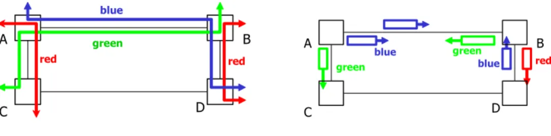
Current solutions include optical circuit switching (OCS) which acts as a solid link between two nodes for long durations. In Figure 2.1(a) an example OCS network is given. There are four source/destination pairs in the topology (A-D,B-D,A-C and B-C) and three different wavelengths are necessary to transfer the associated traffic. Circuit switching first involves a two way reservation process which is called the link set-up phase. The source node sends a request to the network towards the destination node and waits for an acknowledgment. After the optical link is created the data gets transmitted and finally when there is no more data to send, the link is teared down (release phase). OCS is suitable for highly

CHAPTER 2. OPTICAL BURST SWITCHING NETWORKS 10

loaded, steady traffic and guaranties QoS due to the fixed bandwidth reservation. However high bandwidth optical links and large distances between nodes make the two way reservation protocol extremely inefficient for short duration sessions. Optical circuit switching cannot be easily used for transporting bursty Internet traffic since the bandwidth is lost during low or off traffic periods and since OCS introduces too much delay due to frequent set-up/release phases. Another aspect of OCS is its fully transparent switching nature. What this means is that once a link is setup between two nodes, there is no way of interfering with the on going data traffic. The data simply enters the network through an ingress node, traverses through the network without any processing and then finally emerges through the egress node. While the transparency is suitable for steady traffic, it strips OCS from valuable network management features, which are important to handle dynamic traffic.

Another proposed alternative is optical packet switching (OPS). In OPS, an optical packet contains both the header and the data payload, which can be fixed or variable. Unlike OCS, there is no network setup phase, as soon as the data packet is ready, it is sent to the network. In OPS, optical packets are stored and forwarded at each interconnecting node. The node receiving the packet, must first separate the payload and header and buffer the payload until the header is processed either optically or electronically (using O/E conversion). After the necessary processing is finished, the node combines the header and data and sends the packet to the next node, until the destination node is reached. This behavior is closely comparable to the traffic in a classical packet switching network, with the addition of optical processing and buffering. The per hop processing also assures that the available bandwidth can be shared statistically. OPS has some downsides mainly due to current technological limitations. First of all, optical buffer (memory) is not currently available. Instead optical data is sent through fiber delay lines (FDL), which can only induce deterministic and limited delays to the optical packet. The usage of FDLs at each node is necessary due to store-and-forward scheme in effect, which in turn leads to fixed packet length and synchronous switching. Secondly, all optical processing is still not available so the optical header should go through a O/E/O conversion at each node. As the

CHAPTER 2. OPTICAL BURST SWITCHING NETWORKS 11

Control Packet

Burst

Offset time

Node A

Node B

Figure 2.2: Optical burst switching

bandwidth in WDM networks increases this task becomes extremely difficult as the node should process all the headers coming through hundreds of wavelengths in each fiber. Finally, the tight coupling of header and data payload requires strict synchronization and fast processing/switching in the order of µs. An example OPS network can be seen in Figure 2.1(b). On the contrary to the OCS case, if the data is sporadic, only one wavelength is enough to carry the same traffic. Also a source node can send traffic to any destination without experiencing any delay, which is convenient for bursty traffic.

To summarize; OCS can provide steady, QoS guarantied traffic while inducing connection set-up delays and inability to handle bursty traffic. On the other hand, OPS provides mechanisms for efficient and manageable transport of traffic, but is not feasible with the current technology and it may not be realized in the near future since optical processing is far from reality.

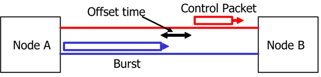
Finally, we have optical burst switching (OBS), which is a recently proposed switching paradigm as described in [12]. OBS lies between optical circuit switch-ing and optical packet switchswitch-ing. OBS has the best of the two worlds: can provide necessary flexibility and efficiency for bursty traffic and is practicable with cur-rent technology. In OBS, the data and control plane are separated, with this hybrid approach control packets are sent over another wavelength and processed electronically at each node. The data burst and it’s related control packet can be seen in Figure 2.2. During transmission the data stays in the optical domain throughout the network topology, so that the network acts as a transparent layer for the transmitted data similar to OCS. But unlike OCS, the core network can

CHAPTER 2. OPTICAL BURST SWITCHING NETWORKS 12

A

B

C

D

20

µ

s

20

µ

s

20

µ

s

cp

burst

Offset time

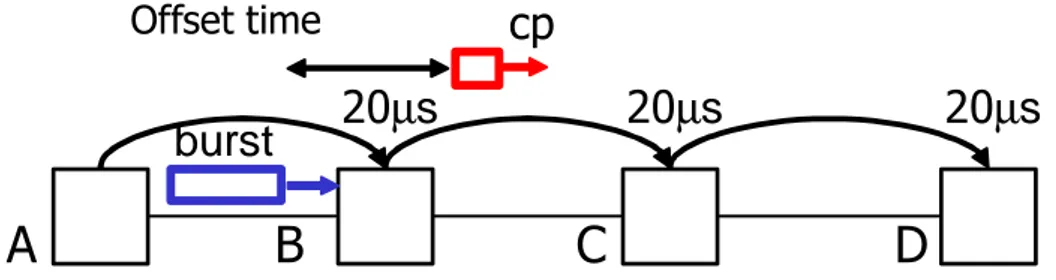
Figure 2.3: Optical burst switching, cp: control packet

still react dynamically to load and topology changes with the usage of out of band control packets. This is an advantage of OBS over OCS. The transparent nature of OBS also redeems the transport layer from the usage of optical buffers, which is the most challenging part of optical data transmission.

In OBS, data from several sources destined to same node are gathered into buffers and are held there until the necessary time or size constraint is reached. In order to overcome the header processing and O/E/O conversion overhead at each node, data packets are aggregated into super packets. If the burst size is chosen to be very small, in the order of several packets, the OBS network will act like an OPS network and the header overhead will be an issue. For instance, if the average burst size is chosen such that each burst consists of 100 data packets, the associated header overhead will be 100 times lesser in OBS compared to OPS. On the other hand, if the burst size is chosen to be very big, more than thousands of packet, the network will act like an OCS network and will not be able to cope with bursty traffic efficiently. After the data payload is aggregated into a data burst, the associated out of band header packet is sent to the network ahead of the burst.

The control packet makes the necessary reservations through the network before the data burst reaches that node so that the burst can pass through without any need for optical buffering. Of course, processing the header at each node will take time, but it must be ensured that the control packet will always stay ahead of the data burst. For example, let’s assume an average header processing time of 20µs at each node and a destination 3 hops away as in Figure 2.3. The control

CHAPTER 2. OPTICAL BURST SWITCHING NETWORKS 13

packet must at least be sent 60µs ahead of the data burst, so that the control packet always stays ahead of the data burst until the destination is reached. This time difference is called the offset-time. After sending the control packet, the source node will wait for an amount of time equaling the calculated offset time and will then send the data burst. This one-way reservation protocol ensures that the data can be transferred between nodes that are far apart without the need to wait for acknowledgements which in turn increases the network utilization greatly.

Finally, the egress node receives the data burst, disseminates the packets and then send them to their appropriate electrical destinations.

2.1.1

Burst Assembly Mechanism

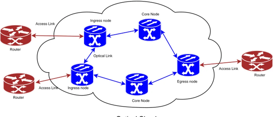
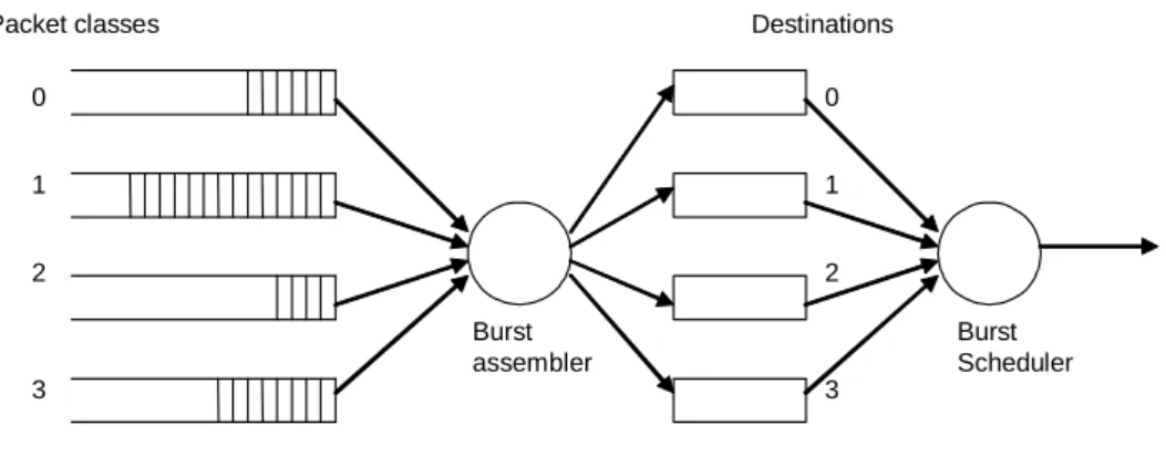
An OBS network consists of ingress nodes, where electronic packets are aggre-gated into optical bursts, core nodes, which act as a transparent transport medium for optical bursts and finally egress nodes, where optical bursts are disseminated to electronic packets. A simple OBS network topology can be observed in Fig-ure 2.4 where red denotes the electrical access links and blue is for optical links. Incoming electronic packets are first aggregated into bursts at ingress nodes. This process is called the burst assembly. There are several methods proposed for this process [15, 16, 17].

In general each node maintains multiple buffers for incoming electronic links from the local network according to their destinations and in some cases for their quality of service requirements as shown in Figure 2.5. Packets from different electronic sources are first stored electronically at the packet queues. Then the burst assembler, arranges the packets according to their destination appropriate burst queues. If QoS is required number of destination queues can be increased to accommodate priority classes. Finally the burst scheduler assigns the burst to their suitable outgoing port and wavelength.

CHAPTER 2. OPTICAL BURST SWITCHING NETWORKS 14 Optical Cloud Egress node Ingress node Ingress node Optical Link Router Access Link Router Router Core Node Core Node Access Link Access Link

Figure 2.4: Optical burst switching network

of packets from the buffers, combine them and send the packets as an optical burst into the core network.

Assembly algorithms use either the assembly time limit or a fixed burst length or both as the decisive factors for burst creation. Parameters involved in the

process are: T the time threshold, B the max burst length and bmin [18], which

stands for the minimum allowable burst size for the particular optical network.

In Fixed-time Min-Length algorithm [15], only bmin and time threshold

is used. Usually bmin is chosen such that bmin < T ∗ λ, where λ is the average

incoming traffic rate. The timer starts when a new packet is received at the empty burst assembly queue. When the pre-set time threshold is reached, the burst is created with the packets waiting at the burst assembly queue. If the burst length

is smaller than the bmin value, packets are padded to satisfy the minimum length

criterion. Fixed-time Min-length algorithm will not act effectively when λ is high, burst will still be influenced by high delay times.

Extending the above algorithm; B, max burst length is introduced according

CHAPTER 2. OPTICAL BURST SWITCHING NETWORKS 15 Packet classes Burst assembler Destinations 0 2 3 1 Burst Scheduler 0 2 3 1 Packet queues

Figure 2.5: Burst assembly architecture

is low and creates an upper bound for the time necessary to create the burst.

B is important especially in high load cases, where B successfully decreases the

unnecessary delays.

The algorithm starts with examination of the incoming burst buffer, if there are more than B packets available a burst is created and sent. If not, the assembler starts the timer and waits for incoming bursts. Whenever the time threshold or the maximum burst length threshold is reached a new burst is created and sent.

Padding will also be done when there are less packets then bmin available at the

time of the burst creation.

After the burst is created an out of band control packet is sent ahead of the burst to setup the path and make the necessary reservations for the incoming burst. The control packet (depending on the architecture used) includes infor-mation about the burst size and the time difference between itself and the data burst, which is called the offset time.

There are several schemes involving the timing and methodology to send and receive the control packet, which will be discussed in the reservation schemes and protocols section.

After the predetermined offset-time passes, the data burst is received. If the burst was scheduled, the node is pre-set and the burst passes through the node

CHAPTER 2. OPTICAL BURST SWITCHING NETWORKS 16

transparently using FDL, wavelength conversion, both or none. After the burst passes through, the node will need some time to reconfigure itself for another burst. The time required is called the switching delay. Switching delay can act as the guard time [11], which can be at the beginning and end of the bursts (usually both) and helps to overcome the uncertainties involved in data burst arrival and data burst lengths due to clock drifts between nodes. The guard time is also responsible in correcting the delay variations in different wavelengths and optical matrix configuration times. Finally performance monitoring and optical error correction may need the use of additional delays. So the node is essentially busy for burst length in time + switching delay to effectively transfer a data burst.

2.1.2

Reservation Schemes and Protocols

There are several mechanisms proposed for reservation in optical burst switching [6, 7, 8, 9]. Prominent architectures involve a one-way reservation design thus lessen the long delays induced by round trip times. If instead a two way reser-vation scheme was used, in a usual scenario in OBS of long routes and high link bandwidths; incredible amounts of optical bandwidth would be wasted.

In Tell-And-Wait (TAW), a control packet from the source node travels and reserves bandwidth through the network. If the reservation is successful the destination sends a go-ahead packet to the source so that the transmission can start. Conversely, a negative acknowledgement is sent back, if the scheduling fails.

In Tell-And-Go [6, 7] data packets and control packets traverse the network simultaneously and are tightly coupled in time. At each node the data packet must be delayed until the control packet is processed and the resulting switching is completed, therefore usage of store and forward units for optical data at each node is necessary.

CHAPTER 2. OPTICAL BURST SWITCHING NETWORKS 17

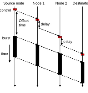
Source node Node 1 Node 2 Destination

delay delay time burst control Offset time

Figure 2.6: JET protocol

A setup packet is used for reserving the bandwidth for incoming burst, the node makes the reservation as soon as the control packet is received. This reservation is valid until a release packet is received.

Finally in Just-Enough-Time (JET) [9, 10] reservation protocol, the control packet reserves the core nodes for a period of time equal to the burst size, starting from the beginning of the burst. Throughout this thesis, JET based reservation scheme will be used. An illustration of JET based scheduling is shown in Fig-ure 2.6. The source nodes which will be sending the data burst, after completing the burst to be sent, creates the control packet and sends it towards the destina-tion node, using a dedicated channel.

Once the control packet is received at the intermediate node, it is transformed into electrical domain and is processed and transformed back into optical domain. This processing is called the optical-electrical-optical (OEO) conversion and the time required for the transformation constitutes the main part of the processing delay. Processing delay also includes the time required to receive and send the control packet. In order to compensate for each delay at each intermediate node, there is a time difference between the control packet and it’s corresponding burst. This number must be large enough so that the control packet always arrives at

CHAPTER 2. OPTICAL BURST SWITCHING NETWORKS 18

a node before the corresponding burst. Time difference is selected to be the product of processing delay at each node by the number of hops the burst will traverse throughout the network and is simply called the offset-time. The offset time may also be deliberately chosen to be bigger than the necessary time. This difference effectively creates a quality of service differentiation amongst different bursts as described in [19, 20, 21].

The offset-time is an important factor in networks using FDLs, as this product, combined with the information of average burst length constitutes the average horizon time [12] of the scheduler. Horizon is the time on the output channel of a core node, after which no scheduled burst exists.

2.2

Contention Resolution in Optical Burst

Switching

In an OBS network, upon receiving the control packet, a node must decide how and when to schedule the incoming data burst and must configure itself accord-ingly. Lack of ability to store the optical data optically (lack of optical memory) and one-way reservation protocols used, makes the task harder. Due to this bufferless property, when multiple bursts content for the same output port, at the same time, for the same wavelength, only one burst can be scheduled and the rest should be dropped. This causes the main disadvantage of optical burst switching, high loss probability. Fortunately any of the parameters that cause contention can be altered so that the overall blocking probabilities may be lower. For contention resolution in wavelength domain, any of the contending bursts can be sent using a different wavelength by means of wavelength converters. The wavelength converters in the network may be sparse and may not always be able to provide full conversion from one frequency to any other frequency.

For time ambiguities, burst can be delayed, not as flexible as an optical mem-ory would have been, but for limited and granular amounts of time. For time

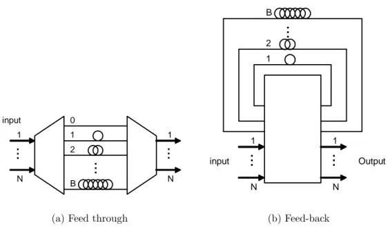
CHAPTER 2. OPTICAL BURST SWITCHING NETWORKS 19

...

...

...

(a) Feed through

input Output

...

...

...

Figure 2.7: An example of FDL modules, Feed through buffering does not support priority routing and feed-back suffers from signal attenuation

delays, bursts are sent into fiber delay loops which are called fiber delay lines (FDLs) [10, 22, 23].

An FDL is simply a fixed length fiber. Once the optical packet enters a fiber, the packet will emerge from the other side after a fixed time delay. The burst can be traversed through several of these long cables, or multiple times from a given fiber cable, providing granular delays from 1 to B times the delay of a single fiber line.

Finally, bursts can be sent to another output port destined to another node, which may or may not be in the initial source-destination route of the incoming burst. This method is called deflection routing and provides limited improvements heavily dependent on the network topology and traffic density as examined in [24]. Deflection routing is not investigated in this thesis.

CHAPTER 2. OPTICAL BURST SWITCHING NETWORKS 20 λ1 λ2 λ3 λ4 time _{t t+D t+2D}

Figure 2.8: First fit algorithm example

2.2.1

Contention Resolution Algorithms

In an OBS environment bursts are usually not received one after another with no interval in between. There are usually certain gaps between the bursts, which are called voids. These voids can be generated during the assembly or scheduling processing also the use of fiber delay lines and different offset-times may cause void generation in between burst. Voids can get wasted as unused channel capacity if an ineffective scheduling algorithm is used. Not all of the contention resolution algorithms in OBS make use of voids and they will be discussed next, starting from simpler ones to more complex ones.

First fit algorithms, in which the incoming burst is just attempted to be scheduled to an outgoing wavelength. This search may be done in a round robin fashion or randomly. In this algorithm, generated voids are totally disregarded, resulting in high drop rates. In the example shown in Figure 2.8; the received burst can be scheduled to λ1, λ2 or λ3.

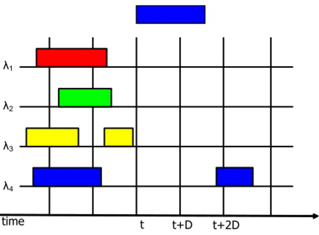
Horizon Scheduling (LAUC) was first proposed by Turner [12]. In this algorithm the scheduler holds track of only the horizon times for each wavelength, where horizon stands for the time of the scheduler after which no reservation exists. The scheduler has access to a FDL buffer which can delay a burst by

CHAPTER 2. OPTICAL BURST SWITCHING NETWORKS 21 λ1 λ2 λ3 λ4 t t+D t+2D t+3D void

Figure 2.9: Lauc algorithm example multiples of FDL granularity D from 1 to B.

When a newly incoming burst arrives at the node the scheduler assigns the burst to the latest horizon as long as the burst’s arrival time is larger than the horizon time. If no channel is available, then the received burst is delayed by a multiple of FDL units until a suitable unscheduled channel is found. If even after maximum number of FDL units is used and no channel is found, the burst is simply dropped.

Trying to find the latest available data channel decreases the lengths of voids generated by the scheduling process. However discounting the voids, causes low utilization and high drop rates.

Figure 2.9 shows an example of LAUC algorithm. The incoming burst arrives at time t. Unable to find an immediate suitable wavelength, the scheduler makes use of FDLs one by one until a suitable unscheduled channel is found. In the first

incrementation, λ2 is found to be accessible and the burst is scheduled.

LAUC-VF [11] is an improved version of LAUC. Unlike LAUC, which only stores the information of horizon time, after which no scheduled burst exist, LAUC-VF also keeps tracks of all available voids in the output port beyond the current time, as well as the information of horizon time. The scheduler has access to an FDL buffer with same properties as the LAUC algorithm.

CHAPTER 2. OPTICAL BURST SWITCHING NETWORKS 22 λ1 λ2 λ3 λ4 Burst Arrival Best Fit Min-SV t t+D t+2D t+3D Min-EV Horizon a b c c

Figure 2.10: Lauc-VF algorithm example

When a control packet arrives at an intermediate node at time t with size L, the scheduler at that node tries to find an output port available for the duration (t to t + L) of the burst. If more than one available channel is found the scheduler selects the latest available data channel, to minimize the size of the void generated. If none is found, the burst is delayed by D and the scheduler looks for an available port for (t + D to t + D + L) time interval. This process goes until an available spot is found are all the FDLs up to B is sought.

There are several criterions in effect depending on the variations of LAUC-VF in use. The first criterion is to find a void interval which minimizes the time difference between the start of the incoming burst and the ending time of the latest scheduled burst and is called the minimum starting void fit (Min-SV). This is also the behavior of the original LAUC-VF [25]. Similarly we can try to minimize the time difference between the end of the incoming burst and the start time of the first scheduled burst, as well as the opposites, namely Max-EV and Max-SV [13]. Finally the burst can be scheduled to the smallest overall void duration, this conduct is called the Best-Fit.

All the variations described above can be observed in Figure 2.10. The newly arriving burst is scheduled to a different wavelength for each condition.

The formal description of the LAUC-VF algorithm is presented below.

CHAPTER 2. OPTICAL BURST SWITCHING NETWORKS 23

channel at time x and returns that value. If a suitable channel is not found, re-turns -1. t is the time of the data burst arrival and j is the outgoing data channel

selected to carry the burst. Finally Qi is the delay induced by the ith FDL.

Begin {LAUC-VF algorithm} Step 1: $i = 0; x=t; Step 2: j = Ch_Search(x);

if (j != -1)

{report the selected data channel j and the selected FDL i; stop; }

else {

i = i + 1; if (i > B)

{report failure in finding an outgoing data channel and stop;}

else

{x = t + Qi, goto Step 2;} }

End {LAUC-VF algorithm}

2.3

Quality of Service in OBS

The increased amount of available bandwidth by means of WDM networks, gave rise to various applications over the Internet demanding quality of service dif-ferentiations. There are four major categories in which quality of service under OBS can be investigated, based on the stage at which the differentiation is per-formed. These are: during assembly-time, reservation, scheduling and finally during contention resolution.

CHAPTER 2. OPTICAL BURST SWITCHING NETWORKS 24

2.3.1

Service Differentiation during Assembly-Time

In this class of QoS schemes, service differentiation requirements are tried to be handled, before the bursts are sent into the network.

The intentional dropping scheme proposed in [26] aims to achieve a propor-tional differentiation between classes. In order to achieve the initially determined burst blocking probabilities, packets from lower priority classes are intentionally dropped such that the percentage of bursts transferred for that specific service class are proportional to the number of bursts transferred from other classes. This scheme does not add any additional delays or does not discriminate between bursts of different sizes. However when the network load is relatively low and the network capacity is enough to handle all of the classes’ QoS requirements, unnec-essary droppings will still be done, leading to performance drops in low priority classes.

2.3.2

Service Differentiation during Reservation

Schemes categorized under this group, create the necessary separation using dif-ferent reservation protocols for difdif-ferent classes.

In offset-time based schemes, bursts with higher priorities are given extra offset-times [27], so that the reservation of higher priority bursts are done before bursts from other priority classes, over the intermediate nodes. Total class iso-lation can be achieved if the offset-time of higher priority class i is chosen to be greater than (maximum burst length + offset time) of a lower priority class j, so that the blocking probability of class i is completely independent of traffic prop-erties of class j [28]. On the other hand, offset-time based schemes add increased end-to-end delays to higher priority classes. Also the excessive creation of voids during reservation disfavors lower priority class bursts with larger sizes.

CHAPTER 2. OPTICAL BURST SWITCHING NETWORKS 25

with lower priorities are created and sent only after the burst is assembled, how-ever control packets of bursts with higher priorities are sent before burst is com-pletely assembled. This in turn creates the class differentiation without inducing additional delay to higher priority bursts. The required information of burst size is filled in using linear predictive filters. If assembled burst’s size is larger then as predicted, a new control packet with the new size information must be sent. The efficiency of this scheme depends on the accuracy of burst size predictions and may not be appropriate for bursty traffic.

The wavelength grouping scheme proposed in [30] restricts the lower priority bursts to certain set of wavelengths while letting higher priority bursts use a larger set or even the complete set of available wavelengths. The difficulty of this scheme rises in the identification of the degree of differentiation between classes of different service requirements.

2.3.3

Service Differentiation during Scheduling

The classes in this section create the differentiation at intermediate nodes using the burst scheduling mechanisms.

In the slot-based prioritized scheduling proposed in [31], data bursts are sent in units of slots (fixed intervals of time), while the control packets are sent in groups which are carried in one slot. The schedulers chooses the higher priority control packets in a group first, allowing them to have a better chance of finding a free channel. In this scheme, the choice of slot size is of importance for success. A small slot size choice may reduce the scheme to that of a classless system, while a larger selection may create unfair discrimination of lower priority bursts.

CHAPTER 2. OPTICAL BURST SWITCHING NETWORKS 26

2.3.4

Service Differentiation during Contention

Resolu-tion

During contention between two bursts, any of the contending bursts may be seg-mented and the segseg-mented part can be dropped or deflected to another outgoing port. The method proposed in [32] segments only the tail (ending) of bursts, in order to minimize out of sequence packets received at the destination. Having known that packets situated at the tail of a burst will have a greater probability of delay or blocking, packets from classes with different priorities are arranged in a burst with a decreasing order of priority, starting from the highest priority packet situated at the beginning of the burst, up until the lowest priority burst at the ending of the burst. However this method does not provide a fully controllable service differentiation mechanism.

Chapter 3

Loss Analysis in OBS Networks

Utilizing Voids

In this chapter, we first introduce the main problem addressed in the thesis, followed by the description of the simulated topology. We then give details about the simulation parameters. The chapter ends with the explanation of the results and relevant discussions.

3.1

Void Characterization in OBS

OBS as stated earlier, stands between optical circuit switching and optical packet switching. OBS has the best of the two worlds; low overheads and less burden on the switching nodes like circuit switching and high utilization and traffic adapta-tion like packet switching. Nevertheless OBS has its own incapabilities.

The main problem in OBS is the high burst loss probability, which is mainly due to the one-way reservation protocol. In order to decrease the contention be-tween bursts and to increase the utilization; contending or newly received bursts must be scheduled as efficiently as possible so that the intervals between bursts

CHAPTER 3. LOSS ANALYSIS IN OBS NETWORKS 28

would be as small as possible. Lesser idle times (voids) between bursts, success-fully increase the channel utilization.

Due to the working principles of optical burst switching networks; generation of voids between bursts is inevitable. Firstly, the granular structure of optical buffers prevents precise accommodation of newly arriving bursts to the appro-priate output port and wavelength. If use of FDLs is necessary because of a contention in progress, in most of the cases a void equal to or less than FDL granularity will be generated.

Secondly bursts, due to the nature of reservation schemes in use, e.g. JET protocol, will have an offset difference associated with their control packet in transit. A burst may be scheduled to a much further destination on the optical network. When the control packet of the burst in consideration arrives at the first node on its way to the destination node, the control packet will try to schedule the node and inform that a burst will arrive after the offset-time difference. As there are many hops left after the first node, the offset time difference will be large, thus the burst will be scheduled to future time. As we know from [19, 20, 21] this burst will a have high probability of getting scheduled and will be easier to employ. There will also be a void induced between the current time and the start time off the burst as great as (totalhopcount − 1) times processing time.

Most promising contention resolution algorithms exploiting the voids have lower blocking probabilities. In order to fully use the voids generated during scheduling, one must truly understand how and when voids are generated. As stated earlier, there are two possible means of void generation, one is due to the use of FDLs, called FDL induced voids, and the other is due to processing and offset-time differences, called the processing time induced voids.

This thesis focuses on the understanding of void generation mechanisms during scheduling of optical bursts. We present the relationship of burst size choices with generated void sizes and density in other to exploit the generated voids to full extent and decrease the blocking probability for bursts of different sizes. Using the void size distribution of an OBS network with given parameters, we can decide which bursts will be favored by void filling scheduling algorithms and which bursts

CHAPTER 3. LOSS ANALYSIS IN OBS NETWORKS 29

will not be able to utilize voids, by simply altering the bursts sizes according to the investigated network’s void size distributions. This decision can easily be used to create a class differentiation between bursts of different sizes and will let us create a simple burst size dependent QoS mechanism.

3.2

OBS Simulator

Optical burst switching due to the inherent behavior does not have many simu-lation environments readily available for use. One solution could be the commer-cially available OPNET software, one can also use the ns2 simulation environ-ment.

ns2 proves to be a powerful tool for network simulations. Most of the protocols

necessary for both wired and wireless networks are readily available; unfortunately optical burst switching is not one of the offered.

There are four main parts of an optical burst switching simulator.

• Burst aggregation and dissemination, also the creation and management of

the control layer.

• Multiple packets progressing through one link, as optical burst switching

makes use of multiple wavelengths

• The scheduling and reservation protocols

• Implementation of wavelength converters, fiber delay lines and deflection

routing if used.

For this thesis work, we needed a simple yet powerful tool to fully understand the problem in consideration and to devise a solution without dealing with the induced problems due to other parameters. Hence a simulator was written in Dev-C++ 4.9.9.2 available under the GNU General Public License. The simulator is programmed in such a way that;

CHAPTER 3. LOSS ANALYSIS IN OBS NETWORKS 30

A

B

S D1 D2 _… D10

W=2

Link speed: 10Gb/s / wavelength

Figure 3.1: Burst arrivals, Basic outline of the simulated architecture

• Both LAUC and LAUC-VF are implemented.

• Tell-And-Go and JET Reordering schemes are available.

• Processing time and switching delay are adjustable in automated steps.

• Both the number of FDLs and their granularities are adjustable, scheduling

without FDLs is also possible.

• Number of wavelengths is adjustable.

• The simulator is capable of processing between 4 ∗ 107_{− 8 ∗ 10}7 _bursts/min depending on the parameters used.

3.2.1

Network Topology and Simulation Parameters

In order to investigate the properties of void generation and the correlation be-tween processing time and FDL structure, a simple node architecture is used. The topology used in the simulations is depicted in Figure 3.1. There are 2 sources, namely A and B, contending for the output port at S. Each source creates bursts, destined to D1 to D10. Burst size varies between 10 packets and 190 packets, which in turn means an average length of 100 packets. Each packet consists of 1500bytes of data, thus the average burst length is 100 ∗ 1500 ∗ 8/10Gbit/s = 120

µs. Burst destined to S are not considered in the simulations as only the output

port of S is investigated. Each optical link has a bandwidth of 10Gbit/s and has 2 different wavelengths.

CHAPTER 3. LOSS ANALYSIS IN OBS NETWORKS 31

. . .

τ

τ

τ

Figure 3.2: Burst generation process

Burst inter-arrival times are generated using a poisson process (see Figure 3.2).

The burst size is randomly chosen according to a uniform distribution (τ2 - τ1,

tburst). From the start time of the burst, exponentially distributed idle time

(tidle) is added (τ3 - τ1). The ratio of the idle times are adjusted in accordance the desired arrival rates such that tidle = ρ . tburst, where ρ is the arrival rate.

The rates used throughout the numerical results section, will be the rate of only one optical channel (for example from A to S), thus total rate of traffic going out of node S will always be two times the given rate in the results.

The exponential time difference between the starting times of two subsequent bursts in some cases may be chosen to be smaller than the size of the first burst.

So to say τ3 may be smaller than τ2. In this case the bursts will already be

contending when they arrive at the source node S. This effectively increases the dropping probability of the pure Poisson burst generation process.

Burst traversing through node S can be destined to D1 through D10. At each jump the control packet for a burst will be delayed by a process time. For the simulations various processing times are used, from 10µs to 100µs. So the offset-time for each burst varies from unit processing offset-time to 10 offset-times the processing time, hence with a processing time chosen to be 20µs, average offset-time will be 110µ.

These numbers -summed and individually- play an important role on burst drop rates. If the channel is empty before the burst arrival, a new scheduled burst on the average will create a horizon of 230µs, which consists of the addition of

CHAPTER 3. LOSS ANALYSIS IN OBS NETWORKS 32

110µs (mean of process time) and 120µs (mean of burst length).

When the total FDL delay is greater then the number calculated above, the effect of FDL granularity is much more observable. In these scenarios voids generated are mainly due to FDL delay differences between bursts. Thus we see a decrease in drop rates for bursts smaller than the FDL granularity. We call this steep decrease in drop rates for bursts smaller than burst FDL granularity D, the knee-effect. Result concerning this behavior will be presented in the numerical results section.

The simulator is capable of processing the contenting burst according to LAUC and LAUC-VF. LAUC-VF was proved to be a better performing algorithm so is chosen as the main interest.

CHAPTER 3. LOSS ANALYSIS IN OBS NETWORKS 33

3.3

Numerical Results and Discussions

3.3.1

Effects of FDL Parameters and Number of

Wave-lengths

In order to fully understand the results in the following sections, we must have an understanding of the underlying properties of optical burst switching networks. The effects of number of wavelengths used in scheduling, FDL granularity and number, on burst loss probabilities are investigated.

Throughout the thesis the following terms will be used:

NF DL Number of FDL buffers

D Delay of each FDL unit in terms of µs, also called the FDL granularity

Tp Processing delay per node

Ts Switching delay per node

ρ Average utilization per incoming channel W Number of wavelengths per link

The simulations only use 2 wavelengths per channel, since the incoming burst process is a true Poisson one, increasing the number of wavelengths will give similar results only with much lesser loss probabilities.

In Figure 3.3, the loss probability is plotted as a function of the burst size for different values of W . In the graph the y axis represent the loss probability of bursts with the indicated size in x axis. Increasing the number of available wave-lengths from 2 to 4 decreases the average loss probability 5.85 times. Similarly an increase from 4 to 8 wavelengths will decrease the average loss probability 54.32 times. The decrease in loss probability is due to the fact that when many wave-lengths are used the scheduler has more choices for assignment for an incoming burst.

CHAPTER 3. LOSS ANALYSIS IN OBS NETWORKS 34 0.000001 0.00001 0.0001 0.001 0.01 0.1 1 12 48 84 120 156 192 228 Burst size(µs) L o s s P ro b a b il it y W=2 W=4 W=6 W=8

Figure 3.3: Number of wavelengths vs average loss probability, ρ=40%, NF DL=16,

D=50µs, Tp=50µs, Ts=0µs

Similarly in Figure 3.4 the effect of increased FDL number is graphed. As expected, burst drop rate decreases with increasing number of FDL units. The scheduler has a better range to delay the contending burst in order to find a suitable outgoing wavelength. As observed, for 8 * 50µs FDL case, there is a steep decrease in drop rates before the 50µs burst size limit. The effect diminishes as the number of FDL units decrease. The motivation behind this behavior will be discussed in the next chapter. Figure 3.4 only gives a brief look at the major effect of increased number of FDL units on loss probabilities.

In Figure 3.5, overall loss probabilities for different processing time and FDL unit sizes are presented. Overall loss probability is the ratio of dropped bursts of all sizes over total number of bursts processed. The loss probability for no FDL case is fairly high, 0.290 and 0.251 for processing times of 100µs and 10µs respectively.

CHAPTER 3. LOSS ANALYSIS IN OBS NETWORKS 35 1.00E-03 1.00E-02 1.00E-01 1.00E+00 12 48 84 120 156 192 228 Burst size(µs) L o s s P ro b a b il it y 1*50us 2*50us 3*50us 4*50us 5*50us 6*50us 7*50us 8*50us

Figure 3.4: Total FDL delay vs burst length histogram, ρ=30%, Tp=20µs, Ts=0µs

3.3.2

Effects of Voids on loss Probabilities

This section focuses on the FDL and processing time induced void generation mechanisms and presents an understanding of the effects caused by several pa-rameters. In order to characterize the duration of voids, the histogram of void durations is generated. The void histograms in this section are created as fol-lows: when a new control packet is received at the source node, all the available void sizes at that moment are counted and corresponding numbers in histogram buckets are incremented by 1. The buckets in the histogram is separated by 1µs. Figure 3.6 shows different scenarios with FDL granularity varying from 10µs to 100µs. Number of FDLs used is altered accordingly such that the total FDL delay is maintained at 400µs. Burst loss probabilities seem to stabilize after burst sizes get larger than the fdl granularity; actually this is not the case. In the scenario above, voids generated due to FDL granularity (because of their huge numbers) suppress the effect of offset-time difference induced voids. Void

histograms for D=25µs,NF DL=16 case shown in Figure 3.8 clearly identify the

CHAPTER 3. LOSS ANALYSIS IN OBS NETWORKS 36 1.00E-06 1.00E-05 1.00E-04 1.00E-03 1.00E-02 1.00E-01 1.00E+00 100 200 400 800 1600 Total fdl delay(µs) L o s s P ro b a b il it y Tp=100µs,No FDL Tp=10µs,No FDL Tp=100µs,D=50µs Tp=100µs,D=25µs Tp=10µs,D=50µs Tp=10µs,D=25µs

Figure 3.5: Total Fdl delay vs Overall Loss Probability, ρ=30%, Ts=0µs

Average loss probability decreases, when a smaller FDL granularity is chosen. Smaller FDL sizes, enable the scheduler to move the burst with greater precision along the output port. This in turn increases the void filling utilization thus decreases drop rates.

In the condition where the total FDL delay is smaller than the mean horizon time, the number of voids generated with offset-time differences are much more obvious. Also there is an increase in average loss probability in contrast to the case with total FDL delay of 400µs. This behavior is shown in Figure 3.7.

In Figure 3.7, total FDL delay of 100µs is selected with varying FDL granu-larities of 10µ, 25µ, 50µ and 100µ. Void sizes are mainly governed by the process delay which can be observed in Figure 3.8. In comparison, when the total FDL delay is smaller, number of voids generated due to FDL granularity is also smaller, which sequentially increases the effect of processing delay.

Finally, the void generation effect of offset-time differences alone is depicted in Figure 3.9. Unlike the FDL granularity induced voids, there is no linear corre-lation between void sizes and drop rates. This exponential behavior may be used

CHAPTER 3. LOSS ANALYSIS IN OBS NETWORKS 37 0 0.005 0.01 0.015 0.02 0.025 0.03 12 48 84 120 156 192 228 Burst size(µs) L o s s P ro b a b il it y Nfdl=40,D=10µs Nfdl=16,D=25µs Nfdl=8,D=50µs Nfdl=4,D=100µs

Figure 3.6: Loss Probability vs Burst Size for total FDL delay of 400µs, ρ=30%,

Tp=20µs, Ts=0µs

to create high QoS differentiation between various burst sizes. Without the use of FDLs, the effect of processing time is much more obvious. Ideally a burst which is destined to the nearest node, arriving just after the scheduling of a burst destined to the farthest node creates the situation of the highest schedulable void filling. This number is calculated by max hop (10) minus min hop (1) multiplied by the processing delay. Bursts bigger than the “process time, hop multiplication” will not see the benefits of void filling, thus bursts bigger than this threshold will all have the same drop rates. Figure 3.10 depicts the loss probability flattening points after which loss probabilities converge to the same value. They are all in concurrence with the multiplication of hop difference with processing time.

In Figure 3.10, we also observe that as Tp increases the overall loss probability

increases. A higher value of Tp increases the mean horizon time and decreases

the ability of the FDLs to traverse the contenting burst up until the horizon time

of the scheduler. Number of voids generated also increases as Tp increases, but

is not enough to compensate for the losses associated with FDLs incapability. On the other hand, blockage of bigger bursts will affect the scheduling of smaller