ADAPTIVE CONTROL DESIGN FOR NONLINEAR SYSTEMS VIA SUCCESSIVE
APPROXIMATIONS
Naser Babaei
Department of Mechanical Engineering, Gazi University
Celal Bayar Bulvari, Maltepe 06570, Ankara, Turkey
Metin U. Salamci
Department of Mechanical Engineering, Gazi University
Celal Bayar Bulvari, Maltepe 06570, Ankara, Turkey
Ahmet Hakan Karakurt
Department Of Mechanical Engineering, Bilkent University
06500, Ankara, Turkey
ABSTRACT
The paper presents an approach to the Model Reference Adaptive Control (MRAC) design for nonlinear dynamical systems. A nonlinear reference system is considered such that its response is designed to be stable via Successive Approximation Approach (SAA). Having designed the stable reference model through the SAA, MRAC is then formulated for nonlinear plant dynamics with a new adaptation rule to guarantee the convergence of the nonlinear plant response to that of the response of the nonlinear reference model. The proposed design methodology is illustrated with examples for different case studies.
INTRODUCTION
Model Reference Adaptive Control (MRAC) design methodologies are studied for dynamical systems in frequency and time domains [1-5]. In general, a Linear Time Invariant (LTI) system is considered as a reference model whose response is the one to be followed by an unknown dynamical system. The control of the plant is established with the MRAC by using a suitable adaptation mechanism. The selection of the LTI reference model is mainly due to its stability property, which is guaranteed by the closed loop eigenvalues of the reference model. In addition, based on the LTI reference model, the adaptation rule can also be generated easily through some specified assumptions (see [1-5] and references therein).
Provided that its stability is ensured, a nonlinear reference model could also be utilized. The advantages of using nonlinear
reference model (instead of LTI one) are studied in [6-8]. It is stated that the adaptation of a nonlinear plant response to the response of a nonlinear reference model may be faster than to that of an LTI reference model [6-8]. The critical issue is that a stable nonlinear reference model is to be assigned so that the response of a dynamical (presumably nonlinear) system converges to the response of the stable nonlinear reference model. There are some approaches to create a stable nonlinear reference dynamics such as State Dependent Riccati Equation (SDRE) approach [6, 9] and Successive Approximation Approach (SAA) [10-12]. Among these publications, SDRE is combined with MRAC in [8] to design personalized drugs for cancer treatment and SAA is extended to MRAC design in [12]. In SAA methodology, the nonlinear system model is approximated as a sequence of linear time varying (LTV) dynamical systems, whose controller can be designed by the classical control approaches developed for the linear systems. The convergence of solutions of the LTV approximations to the solution of the nonlinear system has been proved in the literature (see [10 and 11] and references therein). Although extensive approaches like SDRE and SAA methodologies have been used successively to control several nonlinear problems, uncertain parameters or unmodeled dynamics may be encountered during practice.
SAA is also synthesized with MRAC to control nonlinear dynamics of Multiple Input Multiple Output (MIMO) systems in [13]. In [13], it is assumed that the parameters and dynamics of the plant are the key in compounding SAA with MRAC, therefore, the optimal solution for the reference model is found first by using SAA. Then known plant dynamics is considered as Proceedings of the ASME 2017 Dynamic Systems and Control Conference DSCC2017 October 11-13, 2017, Tysons, Virginia, USA
DSCC2017-5353
a sequence of LTV approximations and the LTV plant approximation with MRAC is stabilized. Thus, it proved that the solution of MRAC for LTV approximations approaches to the solution of the MRAC for nonlinear plant. All these procedures are done by considering fully known plant dynamics, which may violate the general assumptions of MRAC.
In this paper, the assumption of known parameters in the plant dynamics is relaxed. The stability problem of the nonlinear reference model is reduced to the stabilizing controller design problem by using LTV approximations. The Linear Quadratic Regulator (LQR) scheme is utilized for this purpose. Then, the solution of the approximation of the reference model is considered as a reference model (trajectory) to MRAC approach for the stabilization of an unknown nonlinear plant.
The rest of the paper is organized as follows: Section 2 presents a basic overview of the SAA control methodology for nonlinear dynamics. Section 3 describes the main result of this paper, in which a new adaptation rule is derived for nonlinear systems. The methodology is illustrated with simulations in Section 4. Section 5 provides conclusions.
SAA FOR NONLINEAR SYSTEMS: BACKGROUND LTV approximations for nonlinear systems is studied in [10, 11] for different controller designs. Consider the following general nonlinear system,
̇ = ( ) + ( ) ( ), (0) = ∈ ℝ .
(1) The nonlinear system (1) may be represented in the so-called “pseudo-linear” form as,
̇ = ( ) ( ) + ( ) ( ), (0) = ∈ ℝ
(2) where ( ) ∈ ℝ × and ( ) ∈ ℝ × are state dependent matrices and are referred to State Dependent Coefficient (SDC) matrices. ∈ ℝ and ∈ ℝ are input and state vectors respectively. The pseudo-linear form allows one to design controller for the nonlinear system by using the design techniques for the linear dynamical systems. For instance, consider the optimal control problem for the following given performance index
= + ∫ [ ( ) ( ) ( ) + ( ) ( ) ( )] (3)
where ( ) ∈ ℝ × and ∈ ℝ × are symmetric positive semi-definite and ( ) ∈ ℝ × is symmetric positive definite matrices. To minimize the performance index of (3) with respect to pseudo-linear form of the nonlinear system (2), we may use the recursive LTV approximations for both the nonlinear system and the cost function. The first approximation is obtained by evaluating the SDC matrices at the initial conditions, which results in the LTI system and related performance index as,
̇[ ]( ) = ( ) [ ]( ) + ( ) [ ]( ), [ ](0) = , (4)
[ ]= [ ] [ ] + ∫ [ ] ( ) [ ]+ [ ] ( ) [ ] , (5)
For the LTI system in the first iteration, = 1, the optimal feedback control can be achieved as follows
[ ]( ) = − [ ] [ ]( ) = − ( ) ( ) [ ] [ ]( ) (6) where [ ] is computed by solving the Algebraic Riccati Equation (ARE)
[ ] ( ) + ( ) [ ]− [ ] ( ) ( ) ( ) [ ]( ) + ( ) = 0 (7) The LTV approximations for > 1 are
̇[ ]( ) = [ ]( ) [ ]( ) + [ ] [ ]( ), [ ](0) = , (8)
[ ]= [ ] [ ] + ∫ [ ] [ ]( ) [ ]+
[ ] [ ]( ) [ ] ,
(9) At each iteration of the approximation sequence with > 1, the problem becomes an LTV optimal control problem. The control of each iteration is given as follows
[ ]( ) = − [ ]( ) [ ]( ) = − [ ]( ) [ ]( ) [ ]( ) [ ]( ) (10) where [ ]( ) = [ ]( ) [ ]( ) [ ]( ). The []( ) term is the solution of a sequence of matrix Differential Riccati Equation (DRE)
̇[ ]( ) = − [ ]( ) [ ]( ) − [ ]( ) [ ]( ) +
[ ]( ) [ ]( ) [ ]( ) [ ]( ) [ ]( ) − [ ]( ) ,
[ ] = . (11)
The DRE of (11) is the final value problem, i.e. [ ] = , and should be solved by backward integration. Then the ith closed-loop dynamical system becomes
̇[ ]( ) = [ ]( ) [ ]( ) (12) where
[ ]( ) = [ ]( ) −
[ ] [ ]( ) [ ]( ) [ ]( ) [ ]( ) (13) The solution of a sequence of LTV system converges to the solution of the nonlinear system (2) under some mild conditions, which are formulated in the following theorem.
Theorem 1. Suppose that ( ) and ( ) satisfy the following conditions
1. ( ) ≤ ∀ ∈ ℝ ,
2. ‖ ( ) − ( )‖ ≤ ‖ − ‖ ∀ , ∈ ℝ , 3. ‖ ( ) − ( )‖ ≤ ‖ − ‖ ∀ , ∈ ℝ , 4. ‖ ( )‖ ≤ ∀ ∈ ℝ ,
where ( ( )) is the logarithmic norm of ( ). Then
approximations [ ] and [ ] in (8) and (10) converge to functions
( ) and ( ) in system (2) which minimize (3) over the set of
feedback controls of the form − ( ) ( ) ( ) ( ).
Proof. The proof is given in [10].
The idea of using SAA will be used to create a stable nonlinear dynamics in the next section, which is then used as a reference model in the MRAC design problem.
MRAC DESIGN FOR NONLINEAR SYSTEMS WITH SAA The SAA is extended to MRAC design for the control of nonlinear systems with unknown parameters. Consider a nonlinear reference model in the following pseudo-linear form,
̇ = ( ) ( ) + ( ) ( ), (0) = ∈ ℝ (14) where ( ) ∈ ℝ × and ( ) ∈ ℝ × are completely known SDC matrices. Based on the background given in Section 2, optimal control may be designed for the reference nonlinear system (14) via SAA as follows,
̇ [ ]( ) = [ ]( ) + [ ]( ), [ ](0) = ⋮ ̇ [ ]( ) = [ ] [ ]( ) + [ ] [ ]( ), [ ](0) = , ≥ 1 ̇ [ ]( ) = [ ]( ) [ ]( ) + [ ] [ ]( ), (15) where the full state feedback control for each iteration is
[ ]( ) = − [ ] [ ]( ) [ ] (16) where [ ]( ) = [ ] [ ] [ ]( ) and []( ) is the solution of a sequence of DRE, as given in (11).
We can represent the closed-loop nonlinear reference model dynamics as follows,
̇ [ ]( ) = ( ) [ ]( ) (17) where [ ], [ ] = [ ] − [ ] [ ] [ ].
By Theorem 1, the solution of sequence of LTV approximations approaches to the solution of nonlinear dynamic of (14). Therefore, we may consider the last iteration of (15) as the reference model and its states as the reference states to be followed by the plant. Then, the following unforced LTV system, with the desired trajectory, is considered as the reference model
̇ ( ) = ( ) ( ) (18)
Corollary 1 Matrix ( ) ∈ ℝ × is bounded and
uniformly stable, that is ( ) ≤ , ∀ ≥ 0, where < ∞ is a
constant.
Consider now the nonlinear plant dynamics given by (1), in which ( ) ∈ ℝ × and ( ) ∈ ℝ × and we assume that the input matrix of ( ) is known and the nonlinear term of ( ) is unknown. In addition, we assume that all states of (1) are measureable. One could represent the plant dynamics in the pseudo-linear form as defined by (2), in which the ( ) ∈ ℝ × is assumed to be unknown state matrix. The known ( ) matrix may be represented as a collection of constant and nonlinear
( ) matrices as follows,
( ) = + ( ), = (0). (19) For known ( ) and ( ) matrices, perfect model following may be achieved with the following controller,
( ) = − ∗( ) ( ) (20)
Assumption 1 There exists an ideal gain matrix, ∗( ) ∈
ℝ × , that results in perfect matching between the reference
model and the plant such that
( ) − ( ) ∗( ) = ( )( ) (21) where ( ) ∈ ℝ × is uniformly stable (Hurwitz) matrix for
all ≥ 0 which is obtained from the last iteration of SAA.
It should be noted that the exact values of the gains ∗( ) is not required, but its existence is essential.
Assumption 2 We assume that ∗( ) is continuously
differentiable, and its derivative is uniformly bounded, ̇∗( ) ≤
< ∞ for all ≥ 0.
Since ( ) matrix is not known exactly, we use estimation of ∗( ) in (20) in the adaptive control
( ) = − ( ) ( ) (22)
where ( ) is the estimate of the ideal ∗( ) in (20). On the other hand, the following state and control parameter errors are considered; ( ) ≜ ( ) − ( ), ( ) ≜ ( ) − ∗( ) ; ( ) ≜
( ) − . Substituting (22) into (2) yields the following closed-loop dynamics
̇ ( ) = ( ) ( ) + ( ) ( ) + ∗( ) ( )
̇ ( ) = ( ) ( ) + ( ) ( ) ( ), (0) = , ≥ 0. (23) By adding and subtracting ( ) ( ) to the right-hand side of (23), the state tracking error dynamics is obtained as
̇( ) = ̇ ( ) − ̇ ( ) = ( ) ( ) + ( ) ( ) ( ), (0) = = −
, ≥ 0. (24)
In addition, the control parameter error dynamics and ( ) matrix virtual errors are
Now consider the following positive definite Lyapunov function candidate,
( ), ( ), ( ) = ( ) ( ) ( ) + ( ) ( ) +
( ) ( ) ( ) ( ) (26)
where ( ) is the symmetric positive definite matrix, that satisfies the following Differential Lyapunov Equation for some
( ) = ( ) > 0,
( ) ( ) + ( ) ( ) + ̇ ( ) = − ( ) (27) The time derivative of the Lyapunov function along the error trajectories is
̇ ( ), ( ), ( ) = − ( ) ( ) ( ) + 2 ( ) ( ) ( ) ( ) ( ) +
2 ( ) ̇ ( ) + ( ) ( ) ( ) ̇ ( ) +
( ) ( ) ( ) ̇ ( ) ( ) (28)
The adaptation rule is then obtained from,
( ) ( ) ( ) ( ) ( ) + ( ) ̇ ( ) + ( ) ( ) ( ) ̇ ( ) + ( ) ( ) ( ) ̇ ( ) ( ) = 0 which gives ̇ ( ) + ( ) ( ) ( ) ( ) ̇( ) ( ) = − ( ) ( ) ( ) ( ) ( ) ( ) (29) One can separate equation (29) into two differential equations based on ( ) and ( ) as follows,
̇ ( ) + ( ) ( ) ( ) ( ) ̇ ( ) ( ) = ( ) ( ) ( ) ( ) ( ) ( ) (30) ̇∗( ) + ( ) 1 + ( ) ( ) ( ) ̇ ( ) ∗( ) = (1 − ) − ( ) ( ) ( ) ( ) 1 + ( ) ( ) (31) where ∈ [1, ∞ ). The following theorem is the main result of this paper, which summarizes the new adaptation rule for the nonlinear system.
Theorem 2. The nonlinear plant dynamics ̇ = ( ) + ( ) , (0) = , ≥ 0 and the controller ( ) = − ( ) ( )
together with the adaptation law
̇ ( ) + ( ) 1 + ( ) ( ) ( ) ̇ ( ) ( ) = − ( ) ( ) ( ) ( ) 1 + ( ) ( ) , (0) = 0, ≥ 0
guarantees that all closed-loop signals in the error dynamics
including ( ) and ( ) are bounded and that the tracking error
( ) ∈ ℒ and ( ) → 0 as → ∞.
Proof: Using the Lyapunov direct stability method by considering positive definite Lyapunov function candidate in (26), the derivative of the Lyapunov function along the system trajectories together with the control parameter error given in
(29) will be ̇ ( ), ( ), ( ) = − ( ) ( ) ( ) ≤ 0, which
implies that the error signals ( ), ( ), ( ) are bounded.
Then boundedness of ( ), ( ), ( ) imply the boundedness of
̇( ). Further, second derivative of the Lyapunov function
candidate is
̈ ( ), ( ), ( ) = − ̇ ( ) ( ) ( ) − ( ) ( ) ̇( ) ( )
− ( ) ( ) ̇( )
In ̈ ( ( ), ( ), ( )), the ( ),̇( ) and ̇ ( ) are bounded
functions. Also assuming that ( ) is satisfying Lipschitz
conditions, i.e. ∀ , ∈ ℝ, | ( ) − ( )| ≤ | − |, the
boundedness of ( ) is verified. Thus, ̈ ( ( ), ( ), ( )) is
bounded function of time, which implies that ̇ ( ), ( ), ( )
is uniformly continuous. Then, using Barbalats Lemma, one can
verify that ̇ ( ), ( ), ( ) asymptotically tends to zero by
time, which under the assumption of (0) ≠ 0 implies
→ ( ) = 0.
The following section illustrates the application of the new adaptation rule, which is formulated by (30).
ILLUSTRATIVE EXAMPLES
This section elaborates the proposed SAA based MRAC with two examples. In the first example, plant and reference model have similar nonlinear dynamical expressions, but parameters/coefficients are different. In the second example, we use the same reference model of the first example, but we consider structurally different nonlinear plant dynamics. The proposed MRAC design is illustrated with the simulations of the examples.
Example 1. Consider the following nonlinear reference model dynamics
̇ = + ; ̇ = + + 4 + 2 +
We assume that all parameters and model dynamics are known. One of the possible representations of the reference model in the SDC form is as follows
( ) = 1 + 0+ 4 21 , ( ) = 1 By using the SAA, we first design optimal control for the nonlinear reference model in order to have a desirable reference response to be followed by the nonlinear dynamical system. In the optimal control design stage, the following non-quadratic performance index is considered to be minimized by the control action.
=1
2 +
1
2 [ ( ) ( ) ( ) + ( ) ( ) ( )]
In this problem, the following constant weighting matrices are considered = 10 0
0 50 and = 1. Therefore, at each iteration, we shall solve the finite value problem of the following DRE,
̇[ ]= − [ ] [ ] − [ ] [ ]( )
+ [ ]( ) [ ] 1 [ ] [ ]− 10 0
0 50
Figure 1. Approximations of the first and second states of the reference model with SAA and nonlinear solution.
The final-value matrix differential Riccati equations are solved in the time interval of = [0 6] via backward integration.
Final-value of [ ]( ) at each iteration is taken as = [ ] = [ ](6) = 5 0
0 5 .
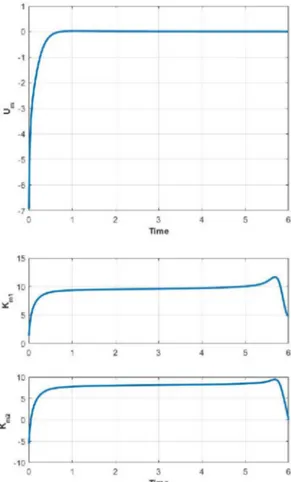
The initial conditions for the simulations are, (0) = [1, − 1] . The solution of LTV approximations converge to the solution of the nonlinear system. The simulation results for the reference model are depicted in Fig. 1. It is seen that the approximations converge to the solution of the nonlinear reference system and the 10th approximation almost fit in the solution of the nonlinear system. Figure 2 shows the control input and control gains of the reference model respectively. It should be noted that the presented control input in Fig. 2 is the control input of the 10th iteration of the approximations, which is the desired optimal control input to stabilize the nonlinear reference model.
Figure 2. Control input and control gains of the reference model with SAA for the last (10th) iteration.
Now consider the following plant nonlinear dynamics, which is similar to the reference nonlinear model but having different parameters.
The following SDC representation is used for the plant dynamics. ( ) = 0 3 2 + 3 + 2 5 , ( ) = 1 3
The positive definite matrix in the Lyapunov Equation, , is considered to be as = 20 0
0 1. We assume that the ( ) is unknown but ( ) is known. Then we split the matrix as ( ) =
+ ( ) = 1 0 + 0 3 which yields ( ) = 0 0 0 3. Then, we can derive the adaptation rule as follows
Δ( ) ≜ 1 + ( ) ( ) = 1 + [0 3 ] 0 3 = 1 + 9 Π ( ) ≜ ( ) ( ) ̇( ) = [0 3 ] 0 0 0 3 ̇ ̇ = 9 ̇ ̇ ( ) + ( ) ( ) ( ) = ( ) ( ) ( ) ( ) ( ) Then ̇ ( ) + ̇ ( ) = ( ) ( ) ( ) ( ). We consider = 1.5, then ̇ ( ) + 9 ̇ 1 + 9 ( ) = 1.5 − ( ) ( ) ( ) ( ) 1 + 9
Figure 3. First and second states of plant with MRAC by considering adaptation rates of 100 and 1000.
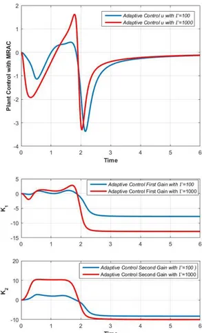
The numerical solutions related to the plant control whit the proposed MRAC are illustrated in Figures 3-4. The states of the plant using two different adaptation rates of 100 and 1000 are given in Fig. 3. Adaptive control input and control gains are depicted in Fig. 4. It is clearly seen that the proposed SAA based MRAC is capable of controlling the nonlinear plant dynamics.
Figure 4. Plant control input and control gains with MRAC by considering adaptation rates of 100 and 1000.
Example 2. Consider now the same nonlinear reference model dynamics as in example 1. However, we consider structurally different nonlinear plant dynamics for the second case study. The new nonlinear plant dynamics is given as follows,
̇ = 5 + (2 + 0.5) ; ̇ = 2 + 2 + 5 + (2 − 4 +
3 )
We choose the following SDC representation for the plant,
( ) = 2 + 20 55 , ( ) = 2 + 0.5
2 − 4 + 3
Also we consider the following positive semi-definite, state dependent matrix for the Lyapunov equation, ( ) =
0
known. Then, ( ) = + ( ) = 0.5 0 +
2
2 − 4 + 3 and
therefore, ( )= − 12 2+ 3 2 + 60 which yields,
1 + ( ) ( ) = 1 + [2 2 − 4 + 3 ] 2 2 − 4 + 3 = 1 + 4 + (2 − 4 + 3 ) ≜ Δ( ) Then, ( ) ( ) ̇ ( ) = [2 2 − 4 + 3 ] 2 0 − 12 + 3 2 + 6 ̇ ̇ = 4 ̇ + (2 − 4 + 3 ){(− 12 + 3 ) ̇ + (2 + 6 ) ̇ } ≜ Π( )
Figure 5. First and second states of plant with MRAC by considering adaptation rates of 100 and 1000.
Then, we can construct the following differential equation for ( ) as ̇ ( ) + ( )( ) ( ) = ( ) ( ) ( )( ) ( ). By considering = 1.5, the following adaptation rule is obtained
̇ ( ) + Π( )
Δ( ) ( ) = 1.5
− ( ) ( ) ( ) ( )
Δ( )
The numerical results for evaluation of the plant states are shown in Fig. 5 with two different adaptation rates of 100 and
1000. Increasing the adaptation rate, a quicker stabilization may be reached. Fig. 6 illustrates the MRAC control input and the adaptive control gains for the plant with two adaptation rates of 100 and 1000. The second case study reveals that the proposed MRAC approach is also capable of controlling the nonlinear plant with structurally different dynamics.
Figure 6. Plant control input and control gains with MRAC by considering adaptation rates of 100 and 1000.
CONCLUSIONS
In this paper, a new MRAC methodology is introduced for a general class of nonlinear systems. The method is based on nonlinear reference model whose stability is designed by using SAA. The proposed MRAC derives a new adaptation rule to force the response of the plant to that of the nonlinear reference model. The proposed method is illustrated with two examples giving the capabilities of the proposed SAA based MRAC. The SAA based MRAC method studied in this paper is extended to drug delivery design for cancer treatment in [14]. The physical implementations of the proposed methodology will be the future study.
[1] Åström, K. J., and Wittenmark, B., 1995, “Adaptive Control”, 2nd ed., Addison-Wesley. MA, USA.
[2] Narendra, K. S., and Annaswamy, A., 1988, “Stable Adaptive Systems”, Prentice Hall, NJ, USA.
[3] Tao, G., 2003, “Adaptive Control Design and Analysis”, Wiley, New York.
[4] Krstic, M., Kanellakopoulos, I., and Kokotovic, P., 1995, “Nonlinear and Adaptive Control Design”, Wiley, New York.
[5] Slotine J. J. E., and Li, W., 1991, “Applied Nonlinear Control”, New Jersey: Prentice-Hall, pp. 242-244, 276-307. [6] Babaei, N., and Salamci, M. U., 2013, “State Dependent Riccati Equation Based Model Reference Adaptive Control Design for Nonlinear Systems,” in Proc. 24th International
Conference on Information, Communication and
Automation Technologies (ICAT), Sarajevo, Bosnia and Herzegovina,.
[7] Babaei, N. and Salamci, M. U., 2014, “State dependent Riccati equation based model reference adaptive stabilization of nonlinear systems with application to cancer treatment”, Proceedings of the 19th IFAC World Congress, Cape Town, South Africa.
[8] Babaei, N. and Salamci, M. U., 2015, “Personalized drug administration for cancer treatment using Model Reference Adaptive Control”, Journal of Theoretical Biology, vol. 371, pp.24-44.
[9] Çimen, T., 2011, “Systematic and effective design of nonlinear feedback controllers via the state-dependent Riccati equation (SDRE) method”, Annual Reviews in Control, vol. 34(1), pp.32-51.
[10] Rodriguez, M. T. and Banks, S. P., 2010, “Linear, time-varying approximations to nonlinear dynamical systems with applications in control and optimization”. Springer-Verlag, Berlin Heidelberg.
[11] Salamci, M. U., Ozgoren M. K., and Banks S. P., 2000, “Sliding Mode Control with Optimal Sliding Surfaces for Missile Autopilot Design,” Journal of Guidance, Control, and Dynamics, vol. 23, no. 4, pp.719-727.
[12] Kodalak, F., and Salamci, M. U., 2015, “Successive Approximations of Model Reference Adaptive Control Design for Nonlinear Systems”, IFAC-PapersOnLine, vol. 48 (25), pp. 248-253.
[13] Babaei, N. and Salamci, M. U., 2015, “Model Reference Adaptive Control for MIMO nonlinear systems by using linear time varying approximation”, 16th International Carpathian Control Conference (ICCC), pp.7-12.
[14] Babaei, N., and Salamci, M. U., “Controller Design for Personalized Drug Administration in Cancer Therapy: Successive Approximation Approach”, Journal of Optimal Control: Applications and Methods, submitted for publication.