Ŕ Periodica Polytechnica
Civil Engineering
59(3), pp. 249–265, 2015 DOI: 10.3311/PPci.7624 Creative Commons Attribution
RESEARCH ARTICLE
Modelling Marshall Design Test Results
of Polypropylene Modified Asphalt by
Genetic Programming Techniques
Serkan Tapkın, Abdulkadir Çevik, Ün U¸sar, Ahmet Kurto˘glu
Received 15-07-2014, revised 14-12-2014, accepted 16-02-2015
Abstract
Determining Marshall design test results is time consum-ing. If the researchers can obtain stability and flow values by mechanical testing, rest of the calculations will just be mathematical manipulations. Marshall stability and flow tests were carried out on specimens fabricated with different type of polypropylene fibers. It has been shown that addition of polypropylene fibers improved Marshall stabilities and Marshall quotient values in a considerable manner. Input variables in the developed genetic programming model use the physical prop-erties of standard Marshall specimens such as polypropylene type, polypropylene percentage, bitumen percentage, specimen height, calculated unit weight, voids in mineral aggregate, voids filled with asphalt and air voids. Performance of the genetic pro-gramming model is quite satisfactory. Besides, to obtain main effects plot, a wide range of parametric studies have been per-formed. The presented closed form solution will also help fur-ther researchers willing to perform similar studies, without car-rying out destructive tests.
Keywords
Polypropylene fibers · Asphalt · Marshall design · Genetic programming · Closed form solutions
Serkan Tapkın
Istanbul Geli¸sim University, Civil Engineering Department, Istanbul, Turkey e-mail: [email protected]
Abdulkadir Çevik
University of Gaziantep, Civil Engineering Department, Gaziantep, Turkey e-mail: [email protected]
Ün U ¸sar
Anadolu University, Civil Engineering Department, Eski¸sehir, Turkey e-mail: [email protected]
Ahmet Kurto ˘glu
Zirve University, Civil Engineering Department, Gaziantep, Turkey e-mail: [email protected]
1 Introduction
Bruce Marshall developed the very basic fundamentals of the Marshall design [1,2]. In 1948, the U.S. Corps of Engineers, im-proved and built up the certain milestones to Marshall’s test pro-cedure [1]. Since this time, Marshall design has been adopted by organisations and government departments worldwide with very minor modifications [2].
Marshall method has been widely adopted and is applicable to both highway and airport flexible pavement construction. Mar-shall specimens are prepared by utilising 35 blows for light, 50 blows for medium and 75 blows for heavy traffic conditions [1]. Basically, two mechanical properties, stability and flow, are determined for the asphalt specimens from the standard shall test. The ratio of stability and flow is known as the Mar-shall quotient (MQ). MQ is a sort of pseudo stiffness which is a measure of the material’s resistance to permanent deformation. More scientifically speaking, MQ is a sort of measure for the creep stiffness of asphalt specimens [3].
The testing procedure in order to determine the optimum bi-tumen contents is very time consuming and needs skilled work-manship. On the other hand, at the end of the Marshall test only stability and flow values of the specimens can be obtained phys-ically. The calculated unit weight of mixture, theoretical unit weight, voids in mineral aggregate (V MA), voids filled with as-phalt (Vf) and air voids (Va) are obtained by carrying out further
calculations. Therefore if the researchers can obtain the stabil-ity and flow values of a standard asphalt mix with the help of other means, the rest of the calculations will just be mathemat-ical manipulations. Genetic programming can be a very con-venient way to model the outcomes of Marshall test procedure. Presenting the main effects plot and a wide range of detailed parametric studies will also help further researchers willing to perform studies on stability, flow and MQ estimation for the very well-known Marshall design procedure, without carrying out destructive tests for similar aggregate sources, bitumen, dif-ferent kinds of polymer modification techniques, aggregate gra-dation, mix proportioning, modification technique and labora-tory conditions.
application of polypropylene (PP) fibers in asphalt modification and applications of genetic programming in pavement engineer-ing. Second part gives detailed information about experimen-tal design. Expression trees of stability, flow and MQ is given in the next section. In order to obtain the main effects plot, a wide range of parametric study has been performed by using the genetic programming models. The analysis of these results is presented next. Finally, the MATLAB codes for the closed form solutions of stability, flow and MQ are given in the Appendices A, B and C respectively.
2 Literature on PP fiber modification and genetic pro-gramming
Studies published about various types of fiber modification of asphalt can be found in relevant literature [4, 5]. Tapkı N has found that dry basis PP modification of asphalt changes the be-haviour of the mixture in a very positive manner [6]. Tapkı N et al. have also worked on the addition of PP fibers to asphalt on a wet basis, and have shown that the most suitable PP fiber type was multifilament, 3 mm long (M-03 type) [7]. In another study by Tapkı N and Özcan, the optimal PP fiber addition amount was determined by the aid of mechanical and optical means [8].
There are various but limited number of studies which utilise genetic algorithms and genetic programming techniques in pavement engineering applications. Sundin & Braban-Ledoux have summarized the findings of up-to-date research articles concerning the application of artificial intelligence to pavement management [9]. Chan et al. have tried to solve the problem of pavement maintenance management at the network level using techniques like mathematical programming and heuristic meth-ods such as genetic algorithms [10]. Tack & Chou have de-scribed in their studies, the development of a genetic algorithm based optimization tool for determining the optimal multiyear pavement repair schedule [11]. Tsai et al. have demonstrated the applicability of the three-stage Weibull equations that were esti-mated using a genetic algorithm to describe the fatigue damage process using flexural controlled deformation fatigue tests [12]. Tsai et al. have demonstrated the applicability of the genetic al-gorithm to solve nonlinear optimization problems encountered in asphalt pavement design [13]. In another study by Alavi et al., a high-precision model was derived to predict the flow number of dense asphalt mixtures using a novel hybrid method coupling genetic programming and simulated annealing [14].
3 Experimental design
Marshall specimens (the optimum bitumen content that has been determined as 5%) were fabricated by utilising 50 blows (medium traffic conditions). Base bitumen of 50/70 penetration was modified in the laboratory with M-03 type PP fibers.
Gradation limits for wearing course Type 2 had been utilised all throughout the studies [15]. The aggregate was calcareous type crushed stone. Physical properties of the base and 3‰ PP fiber modified bitumen samples by aggregate weight are given
in Table 1. The physical properties of coarse and fine aggre-gates are given in Table 2. The apparent specific gravity of filler is 2790 kg/m3. The mixture gradation is being given in Table 3. Physical properties of the PP fibers used in the experimental pro-gram are given in the relevant literature [4].
Tab. 1. Physical properties of the base and 3 ‰ PP fiber modified bitumen samples by aggregate weight (bold values are for modified bitumen)
Property Test Value Standard
Penetration at 25 °C, 1/10 mm 55.4, 45.5 ASTM D 5-97 Penetration Index -1.2, -0.8 -Ductility at 25 °C, cm >100, >100 ASTM D 113-99
Loss on heating, % 0.057, 0.025 ASTM D 6-80 Specific gravity at 25 °C, kg/m3 1022, 1015 ASTM D 70-76
Softening point, °C 48.0, 52.05 ASTM D 36-95 Flash point, °C 327, 292 ASTM D 92-02 Fire point, °C 376, 345 ASTM D 92-02
Tab. 2. Physical properties of coarse and fine aggregates (bold values are
for fine aggregates)
Property Test Value Standard
Bulk specific 2703, ASTM C 127-04, gravity, kg/m3 2610 ASTM C 128-04
Apparent specific 2730, ASTM C 127-04, gravity, kg/m3 2754 ASTM C 128-04
Water absorption, 0.385, ASTM C 127-04,
% 1.994 ASTM C 128-04
Tab. 3. Type 2 wearing course gradation [15]
Sieve size, mm Gradation limits, % Passing, % Retained, %
12.7 100 100 0 9.52 80-100 90 10 4.76 55-72 63.5 26.5 2.00 36-53 44.5 19.0 0.42 16-28 22 22.5 0.177 8-16 12 10.0 0.074 4-10 7 5 Pan - - 7
PP fibers were premixed with bitumen using a standard mixer at 500 revolutions per minute for two hours. The mixing tem-perature was around 165-170°C [16]. For the sake of testing reasons, the base bitumen samples were also subjected to same temperature to equalise the oxidative and aging effects PP mod-ification. Three types of PP fibers: M-03(with fiber length of 3 mm), M-09 (with fiber length of 9 mm) and waste fibers were used in this research. For M-03 type fibers, fiber contents of 3, 4.5, and 6‰ by weight of aggregate were premixed with bitu-men and were used for preparation of standard Marshall speci-mens [4]. For M-09 type and waste fibers only 3‰ fiber content was utilized as it was really difficult to mix fibers with greater lengths with bitumen using standard mixers. According to the workability criteria, M-03 type fibers were found to be the best
modifiers and, due to the consistency of the Marshall test re-sults, 3‰ fiber content was determined to be the optimal addi-tion amount. With these amounts, PP fibers melt in bitumen and bitumen forms a continuous phase for PP particles which are hung as globules. The physical properties of the PP fiber based bitumen samples with 3‰ fiber content are given in Table 1.
Penetration, penetration index, specific gravity and softening point characteristics of PP modified bitumen samples were im-proved as compared to base bitumen considerably, as depicted in Table 1. Therefore, the addition of 3‰ of M-03 type fibers clearly shows the decrease in temperature susceptibility of the base bitumen.
To determine the optimum bitumen content, Marshall mix de-sign procedure was utilised. The relevant physical and mechan-ical test results are summarized in Tables 4 to 9. The values stated in these tables are the average values for three different specimens. Table 4 represents the Marshall test results of spec-imens prepared with base bitumen. Tables 5 to 7 present the relevant physical and mechanical test results of specimens fab-ricated with utilising M-03 type fiber contents of 3‰, 4.5‰ and 6‰ (by weight of aggregate). Tables 8 and 9 present the rele-vant physical and mechanical test results of specimens with M-09 type fiber at 3‰ contents and waste fibers with fiber content 3‰ (by weight of aggregate).
To determine the optimum bitumen content, the bitumen con-tents corresponding to the mixtures with maximum stability and unit weight, 4% Va and 70% Vf, were found and averaged
ac-cording to the limits [15]. These optimum bitumen contents are represented in Fig. 1.
Fig. 1. Optimum bitumen content values
Based on the performed experiments, the optimum bitumen content varies depending on the type and dosage of fibers. How-ever, the optimal PP amount, the type, the homogeneity in the preparation of the Marshall specimens, the ease in the addition of the PP fibers, the ease in the fabrication of the specimens and the fluctuations of the observed physical and mechanical prop-erties are also very important. For example, specimens prepared with higher dosages of M-03 fibers, mixtures made with M-09 and waste fibers resulted in increased values of optimal bitumen contents. M-09 and waste fibers also had very little workability. The addition of these fibers into bitumen is difficult and results
in very viscous modified bitumen samples that does not allow the fabrication of stable Marshall specimens. The fluctuations in the stability and flow values and MQ values do support the above mentioned observations. Based on these results, M-03 PP fibers at dosage of 3‰ by the weight of aggregates were se-lected as optimal PP addition amount. Also, it can be seen that the optimum bitumen contents for reference and specimens with 3‰ of M-03 fibers are 4.81% and 4.97%, respectively (Fig. 1).
The maximum average stability value of reference mixture was 15620.4 N (Table 4). Mixture with 3‰ of M-09 PP fibers had the maximum average stability value of 22008.6 N (Table 8). However, the Marshall specimens prepared with 3‰ of M-03 PP fibers had 20% increase in the average Marshall stability and according to the workability criteria, chosen as the optimal PP type and addition amount. The PP fiber modification aims to increase the service lives by increasing the stiffness of asphalt specimens. Therefore, the addition of 3‰ of M-03 type fibers clearly shows the decrease in temperature susceptibility of the base bitumen. The noticeable increase of Vavalues is visualized
from Tables 4–9. More air voids values mean better resistance to bleeding problems and formation of rutting especially in hot climates. In dense bituminous mixtures, there is certainly a need for a minimum air void content to avoid binder thermal expan-sion and subsequent bleeding. However, at the first glance, it might seem as if that increasing the air void content above a cer-tain level would lead to post compaction and subsequent rutting (in the form of compression and not plastic deformation). It is evident that PP fibers increase the Va through the mix in dense bituminous mixtures. This increase is probably caused by the in-crease in surface area for the aggregate and PP fibers. Since PP fibers behave as filler materials which need to be wetted by the asphalt binder, lower asphalt (effective asphalt) cannot fill the space between the mineral aggregate and produces the increase in air voids [17]. This finding is also supported by the results of Muniandy and Huat [18]. They have shown that the viscos-ity of fiber reinforced asphalt concrete may be increased by the introduction of fibers to the system. The increase in viscosity can reduce bitumen penetration in the mixture. As Vavalues
in-crease, the unit weight values in all PP fiber reinforced mixtures decrease [17]. After construction, a dense bituminous pavement has air voids in the range of 8%. It is accepted by the researchers that due to the further trafficking, the pavement will get densi-fied to the design air void content of 3 to 5% after a period of 2 to 3 years. However, during this period, ingress of water into the pavement through the interconnected air voids causes moisture induced damage to the asphalt concrete layers[19]. One way to prevent this distress mechanism is to have impervious mixes that will be densified by traffic to a very small extent and this is achieved by laying dense mixes having air voids of the order of 2 to 3%. However, due to damage mechanisms like rutting and bleeding which come into play at very low air voids content, it necessitates the presence of air voids at least of the order of 8% in a virgin asphalt concrete layer [19]. Moreover the increase in
Tab. 4. Physical and mechanical testing results for specimens prepared with base bitumen
Bitumen Content
Unit Weight
(kg/m3) VMA(%) Vf(%) Va(%) Stability (N) Flow (mm)
Marshall Quotient (N/mm) 3.5 % 2368.9 17.0 45.8 8.8 13988.3 2.4 5889.8 4.0 % 2408.3 16.0 56.3 6.7 15251.9 2.6 5927.7 4.5 % 2439.1 15.3 66.6 4.8 15620.4 2.6 6005.5 5.0 % 2449.9 15.4 73.8 3.7 13951.7 2.8 4928.2 5.5 % 2458.3 15.5 80.4 2.7 11581.0 4.5 2594.0 6.0 % 2443.1 16.4 82.0 2.6 9808.4 4.7 2100.8 6.5 % 2427.1 17.3 83.2 2.6 8450.2 5.4 1562.3 7.0 % 2412.8 18.2 84.3 2.5 7191.6 6.9 1043.0
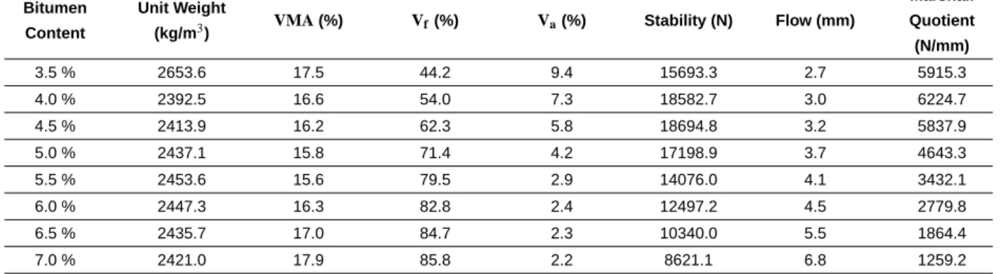
Tab. 5. Physical and mechanical testing results for specimens modified with 3‰ of M-03 type PP fibers
Bitumen Content
Unit Weight
(kg/m3) VMA(%) Vf(%) Va(%) Stability (N) Flow (mm)
Marshall Quotient (N/mm) 3.5 % 2653.6 17.5 44.2 9.4 15693.3 2.7 5915.3 4.0 % 2392.5 16.6 54.0 7.3 18582.7 3.0 6224.7 4.5 % 2413.9 16.2 62.3 5.8 18694.8 3.2 5837.9 5.0 % 2437.1 15.8 71.4 4.2 17198.9 3.7 4643.3 5.5 % 2453.6 15.6 79.5 2.9 14076.0 4.1 3432.1 6.0 % 2447.3 16.3 82.8 2.4 12497.2 4.5 2779.8 6.5 % 2435.7 17.0 84.7 2.3 10340.0 5.5 1864.4 7.0 % 2421.0 17.9 85.8 2.2 8621.1 6.8 1259.2
Tab. 6. Physical and mechanical testing results for specimens modified with 4.5‰ of M-03 type PP fibers
Bitumen Content
Unit Weight
(kg/m3) VMA(%) Vf(%) Va(%) Stability (N) Flow (mm)
Marshall Quotient (N/mm) 3.5 % 2351.1 17.6 43.9 9.5 16289.0 3.6 4532.7 4.0 % 2379.6 17.0 52.3 7.8 18817.3 3.0 6183.1 4.5 % 2388.5 17.1 58.5 6.8 18758.7 3.2 5787.9 5.0 % 2414.0 16.6 67.3 5.1 19670.0 3.2 6066.0 5.5 % 2425.0 16.6 74.0 4.0 14670.3 3.9 3789.1 6.0 % 2418.3 17.3 77.1 3.6 12518.0 4.0 3159.0 6.5 % 2412.8 17.8 80.3 3.2 11460.5 3.8 2982.4 7.0 % 2408.8 18.3 83.5 2.7 9765.5 4.6 2127.4
Tab. 7. Physical and mechanical testing results for specimens modified with 6‰ of M-03 type PP fibers
Bitumen Content
Unit Weight
(kg/m3) VMA(%) Vf(%) Va(%) Stability (N) Flow (mm)
Marshall Quotient (N/mm) 3.5 % 2327.4 18.4 41.5 10.4 16217.6 3.0 5442.8 4.0 % 2352.7 17.9 49.2 8.8 18070.4 2.7 6741.0 4.5 % 2337.6 18.9 52.0 8.7 17168.8 3.5 4914.3 5.0 % 2342.8 19.1 56.9 7.9 17209.7 4.1 4197.2 5.5 % 2404.7 17.3 70.5 4.8 16816.8 3.2 5194.7 6.0 % 2380.5 18.5 70.6 5.1 14282.1 3.7 3879.6 6.5 % 2394.7 18.4 77.1 3.9 13797.5 3.6 3818.1 7.0 % 2374.8 19.5 77.4 4.1 12504.6 5.0 2482.1
Tab. 8. Physical and mechanical testing results for specimens modified with 3‰ of M-09 type PP fibers
Bitumen Content
Unit Weight
(kg/m3) VMA(%) Vf(%) Va(%) Stability (N) Flow (mm)
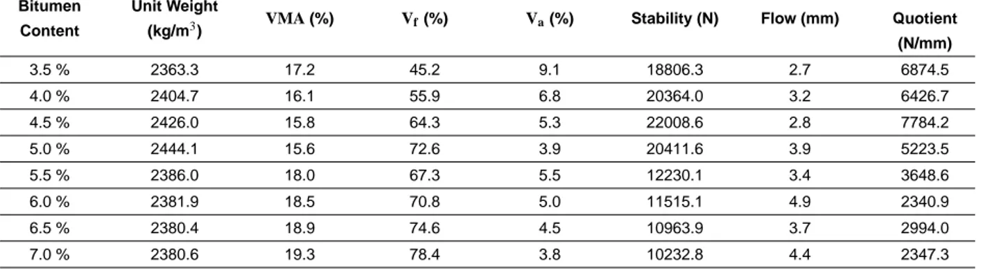
Marshall Quotient (N/mm) 3.5 % 2363.3 17.2 45.2 9.1 18806.3 2.7 6874.5 4.0 % 2404.7 16.1 55.9 6.8 20364.0 3.2 6426.7 4.5 % 2426.0 15.8 64.3 5.3 22008.6 2.8 7784.2 5.0 % 2444.1 15.6 72.6 3.9 20411.6 3.9 5223.5 5.5 % 2386.0 18.0 67.3 5.5 12230.1 3.4 3648.6 6.0 % 2381.9 18.5 70.8 5.0 11515.1 4.9 2340.9 6.5 % 2380.4 18.9 74.6 4.5 10963.9 3.7 2994.0 7.0 % 2380.6 19.3 78.4 3.8 10232.8 4.4 2347.3
Tab. 9. Physical and mechanical testing results for specimens modified with 3‰ of waste PP fibers
Bitumen Content
Unit Weight
(kg/m3) VMA(%) Vf(%) Va(%) Stability (N) Flow (mm)
Marshall Quotient (N/mm) 3.5 % 2360.6 17.3 44.9 9.2 14545.6 3.4 4234.1 4.0 % 2379.0 17.0 52.2 7.8 13937.0 3.7 3780.0 4.5 % 2406.8 16.5 61.2 6.0 14922.4 4.6 3233.2 5.0 % 2434.2 15.9 70.8 4.3 14712.7 3.6 4078.6 5.5 % 2453.9 15.6 79.5 2.8 12729.5 3.7 3397.2 6.0 % 2451.5 16.1 83.7 2.3 9730.6 4.5 2146.5 6.5 % 2434.0 17.1 84.4 2.3 8286.7 5.7 1447.6 7.0 % 2418.4 18.1 85.3 2.3 7254.4 7.2 1008.5
MQ values is very noticeable. Therefore, the PP modification
provides a positive contribution to the overall performance of asphalt pavements.
4 Background on genetic programming (GP)
Genetic algorithm (GA) is an optimization and search tech-nique which is mainly based on the principles of genetics and natural selection. A GA allows a population composed of many individuals to evolve under specified selection rules to a state that maximizes the “fitness” (i.e., minimizes the cost function).
Genetic programming (GP) is an extension to genetic algo-rithms proposed by Koza [20]. Koza defines GP as a domain-independent problem solving approach in which computer pro-grams are evolved to solve, or approximately solve, problems based on the Darwinian principle of reproduction and survival of the fittest and analogs of naturally occurring genetic operations such as crossover (sexual recombination) and mutation. GP re-produces computer programs to solve problems whose flowchart can be found in the relevant literature [20].
4.1 Brief overview of Gene expression programming (GEP) Gene expression programming (GEP) software which is used in this study is an extension to GP that evolves computer pro-grams of different sizes and shapes encoded in linear chromo-somes of fixed length. The chromochromo-somes are composed of mul-tiple genes, each gene encoding a smaller sub-program. Fur-thermore, the structural and functional organization of the linear chromosomes allows the unconstrained operation of important
genetic operators such as mutation, transposition, and recombi-nation. One strength of the GEP approach is that the creation of genetic diversity is extremely simplified as genetic operators work at the chromosome level. Another strength of GEP con-sists of its unique, multigenic nature which allows the evolution of more complex programs composed of several sub-programs. As a result GEP surpasses the old GP system in 100 - 10,000 times [21–23]. APS 3.0, a GEP software developed by Candida Ferreira has been utilised in this study [24].
The fundamental difference between GA, GP and GEP is due to the nature of the individuals: in GAs the individuals are lin-ear strings of fixed length (chromosomes); in GP the individuals are nonlinear entities of different sizes and shapes (parse trees); and in GEP the individuals are encoded as linear strings of fixed length (the genome or chromosomes) which are afterwards ex-pressed as nonlinear entities of different sizes and shapes (i.e., simple diagram representations or expression trees).
5 Numerical Application
The main focus of this study is to explore an application of genetic programming for modelling and presenting closed form solutions to Marshall design test results for wet based PP fiber modified asphalt mixtures. Therefore an extensive laboratory testing and data analysis phase has been performed throughout the study. The details of the experimental database including the ranges of parameters are given in Table 10.
5.1 Results of GP Formulations
The input variables in the developed genetic programming model use the physical properties of standard Marshall speci-mens such as PP type, PP percentage, bitumen percentage, spec-imen height, calculated unit weight, V MA, Vf and Vain order
to predict the Marshall stability, flow and MQ values. Prior to GP modelling, the experimental results are divided into ran-domly selected training and testing sets among the experimen-tal database with 80% and 20%, respectively to prevent over fitting. The GP modelling was performed by GeneXpro-Tools 4 [24]. The GP model was constructed with training sets and the accuracy was verified by testing sets which the GP model faces for the first time. Related parameters for the training of the GP models are given in Table 11. It should be noted that the proposed GP formulation is valid for the ranges of training set given in Table 10. Statistical parameters of test and training sets of GP formulations are presented in Table 12. The GP results versus actual test results for the three different models are rep-resented in Figs. 2–4 for stability, flow and MQ data analyses respectively.
Fig. 2. The genetic programming results versus actual test results for stabil-ity
Fig. 3. The genetic programming results versus actual test results for flow
Fig. 4. The genetic programming results versus actual test results for MQ
The expression tree of stability, flow and MQ obtained from genetic programming software GeneXpro-Tools 4 [24] are shown in Figs. 5–7 respectively where d0, d1, d2, d3, d4, d5,
d6, d7 and d8 correspond to PP type, PP percentage, bitumen
percentage, specimen height, calculated unit weight, V MA, Vf,
Va. The MATLAB codes for the closed form solutions of
sta-bility, flow and MQ are given in The Appendices A, B and C respectively.
6 Parametric studies
The main effects plot is an important graphical tool to visual-ize the independent impact of each variable utilised in the car-ried analyses on stability, flow and MQ values. This tool allows the reader to visualise a better and much simpler snapshot of the overall significance of variable effects on the outputs. In the main effects plot, the mean output is plotted at each factor level which is later connected by a straight line. The slope of the line for each variable is the degree of its effect on the out-put. In order to obtain the main effects plot, a wide range of detailed parametric studies have been performed by utilising the proposed GP model. The main effects plot will also help fur-ther researchers willing to perform studies on stability, flow and
MQ values for the very well-known Marshall design procedure,
without carrying out destructive tests. 6.1 Analysis of results
In this part of the study, analyses of the graphs that have been obtained at the end of parametric studies have been given. First of all the results of the stability analyses is stated out.
6.1.1 Stability analyses
The maximum load the specimen will carry before failure is known as the Marshall stability. In Fig. 8 and the rest of the similar figures all throughout the study, y-axis relates to the out-put values that have been analysed, i.e. stability, flow and MQ. Instead of a detailed analysis of all of the graphs that have been obtained at the end of parametric studies, some of the “very”
Tab. 10. Experimental database ranges PP Type ‰ PP % Bitu-men Spec. height (mm) U.W. Calcu-lated (kg/m3) V M A (%) Vf(%) Va(%) Marshall Quo-tient (kg/mm) Stability (kg) Flow (mm) Max 3.00a 6.00 7.00 62.00 2470.24 19.78 89.45 10.76 886.77 2289.4 7.92 Min. 0.00b 0.00 3.50 58.00 2311.26 14.47 40.70 1.48 92.77 689.52 1.85 Mean 1.15 2.78 5.24 59.86 2408.41 16.98 68.62 5.00 412.64 1396.6 3.96 Std. Dev 1.00 2.05 1.15 1.00 37.63 1.25 14.07 2.51 201.45 387.8 1.38
a denotes PP modified specimens b denotes control specimens
Tab. 11. Parameters of the GEP models
P1 Function Set: +, -, *, /,sqrt, e x, ln(x), Power, Loe2a, Inverse P2 Chromosomes: 30-500 P3 Head Size: 6,8,10 P4 Number of Genes: 3
P5 Linking Function: Addition, Multiplication
P6 Fitness Function Error Type: MAE (Mean Absolute Error), Custom Fitness Function
P7 Mutation Rate: 0.044
P8 Inversion Rate: 0.1
P9 One-Point Recombination Rate: 0.3
P10 Two-Point Recombination Rate: 0.3
P11 Gene Recombination Rate: 0.1
P12 Gene Transposition Rate: 0.1
Tab. 12. Statistical parameters of testing and training sets and overall results of GP models
Training set Testing set Total set
STABILITY MSE 22692.29 20903.22 22107.86 M APE 8.906603 7.772239 8.654942 R2 0.848603 0.807624 0.84731 Mean 1.011132 1.003738 1.008746 COV 0.131207 0.128227 0.129873
Training set Testing set Total set
FLOW MSE 0.599844 0.758636 0.625493 M APE 14.97459 18.49503 15.56552 R2 0.671612 0.466143 0.651925 Mean 1.003448 0.991535 1.000904 COV 0.2064 0.259264 0.215818
Training set Testing set Total set
MSE 7287.673 8117.646 7369.808
MARSHALL M APE 16.54798 16.4854 16.47248
QUOTIENT R2 0.821313 0.745823 0.815734
(MQ) Mean 0.968293 0.999487 0.973579
COV 0.209135 0.197823 0.206148
MS Estands for “mean squared error”,
MAPEstands for “mean absolute percentage error”, COVstands for “coefficient of variation”
Fig. 5. The expression tree of stability obtained from genetic programming software GeneXpro-Tools 5 [24]
Fig. 6. The expression tree of flow obtained from genetic programming softwareGeneXpro-Tools 5 [24]
Fig. 7. The expression tree of MQ obtained from genetic programming soft-ware GeneXpro-Tools 5 [24]
representative interaction plots besides the main effect plots for stability analyses have been presented. All of the presented graphs are important from pavement engineering point of view and present a perfect notification of material property analysis demonstration in a novel manner. Besides, all throughout the analyses, PolType 0 stands for PP modified specimens’ results.
Fig. 8.Interaction plot for PP percentage vs. stability
In Fig. 8, the double effect of the increase in PP percentage and the increase of Va can be clearly observed as a visible
in-crease in stability values.
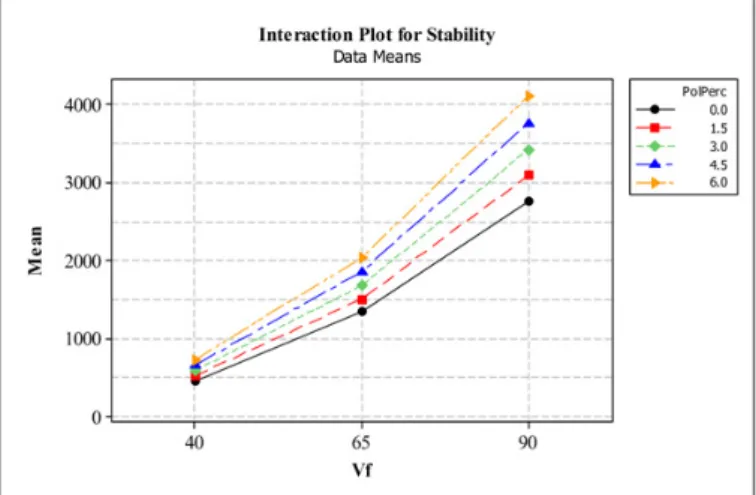
Fig. 9.Interaction plot for Vf vs. stability
In Fig. 9, as the Vf values increase, the stability values also
increase. This is due to the nature of PP fiber modification [4]. Here, it has to be mentioned that Vf is not an independent value.
It is obtained by dividing volume of bitumen into V MA. There-fore, this interesting phenomena comes from these facts. Also as the PP percentage increases, the stability values go along with this increase.
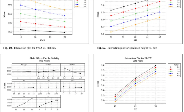
As V MA values go further beyond a level, stability values start to decrease abruptly (please refer to Fig. 10). Also the de-crease in the PP percentage creates a similar effect.
In Fig. 11 the general snapshot of the parametric study of mean effects stability analysis can be visualized in a compact manner.
Fig. 10. Interaction plot for V MA vs. stability
Fig. 11. Whole trends for the parametric study of main effects of stability analysis
6.1.2 Flow analyses
The amount of deformation of the specimen before failure occurs is known as flow. As we utilise PP modification in this study, it is visualized from Figs. 12-15 mainly that the mean flow values increase in a manner just as the bitumen percentage increases which is expectable form materials science point of view.
As the specimen heights increase, flow values also increase as this phenomenon is being considered in the test methods (please refer to Fig. 12). The increase of the PP percentage does not have a considerable effect on flow values as can be clearly seen from the narrow band of results.
The increase in Vf values result in the increase of the flow
values. The increase of the PP percentage does not have a con-siderable effect on flow values as can be clearly seen from the narrow band of results (please refer to Fig. 13).
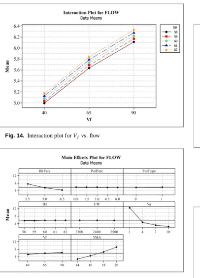
The increase in Vf values result in the increase of the flow
values as can be seen in Fig. 14. As specimen height values increase, the flow values also increase in a similar fashion.
In Fig. 15, the general snapshot of the parametric study of mean effects flow analysis can be visualized in a compact man-ner.
Fig. 12. Interaction plot for specimen height vs. flow
Fig. 13. Interaction plot for Vf vs. flow
6.1.3 Marshall quotient (MQ) analyses
The ratio of stability to flow is known as the MQ. MQ is a measure of the material’s resistance to permanent deformation. From Figs. 16 to 19, the panorama for the MQ values that have been obtained at the end of parametric studies have been given.
The increase in unit weight values end up with more stiff mix-tures as can be seen from the MQ values in Fig. 16. But it has to be borne in mind that this difference is in a narrow band again. Also, introducing more PP ends up with asphalt specimens hav-ing higher MQ values.
A similar argument is valid for V MA values according to the above discussion. Moreover, the increase in Va ends up with
stiffer specimens (please refer to Fig. 17).
When PP addition amount increases, the MQ values also in-crease. The increase in the specimen heights stands for a very similar argument as can be visualised in Fig. 18. As the spec-imen heights increase, MQ values also increase as this phe-nomenon is being considered in the test methods
In Fig. 19 the general snapshot of the parametric study of mean effects flow analysis can be visualized in a compact man-ner.
Fig. 14. Interaction plot for Vf vs. flow
Fig. 15. Whole trends for the parametric study of main effects of flow anal-ysis
7 Conclusions
This paper presents a new and efficient approach for the pre-diction of mechanical properties such as stability, flow and MQ obtained from Marshall design tests utilizing GP for dense bitu-minous mixtures used as wearing course in the pavement struc-ture. The increase in the stability values for the PP modification deserves attention. When Va values are concerned, the
notice-able increase is visualized from the test data. Moreover the in-crease in MQ values is also noticeable. This novel approach is very important in the sense that for a specific type of as-phalt mixture and maximum aggregate size, the stability, flow and MQ values obtained at the end of Marshall design tests can be estimated without carrying out destructive tests which takes too much time and human effort. Moreover, the PP modifica-tion provides a significant contribumodifica-tion to the performance of asphalt pavements which have rutting susceptibility. There are no prior applications of GP to present a closed form solution to the well-known mechanical testing side of Marshall design in the literature in this manner. The results of the proposed GP model are observed to be quite accurate. The GP based models for stability flow and MQ are observed to be very close to actual experimental results. The main outcome of this study is actually to emphasize that GP can be used for modelling of asphalt based
Fig. 16. nteraction plot for unit weight vs. MQ
Fig. 17. Interaction plot for V MA vs. MQ
Fig. 19. Whole trends for the parametric study of main effects of MQ anal-ysis
materials in general. The main advantage of GP over traditional regression techniques is that there is no predefined function to be considered for modelling. GP approach creates randomly formed functions and selects the one that best fits the results. On the other hand, the outcomes of the study are very promising as it will open a new era for the accurate and effective explicit formulation of many pavement engineering problems and will provide very good requirements for airfield asphalt applications where Marshall design is related to especially in CEN/EU coun-tries.
References
1 Mix design methods for asphalt concrete and other hot-mix types, Manual series No 2, The Asphalt Institute, 1988.
2Roberts FL, Mohammad LN, Wang LB, History of hot mix as-phalt mixture design in the United States, Journal of Materials in Civil Engineering, ASCE, 14(4), (2002), 279–293, DOI 10.1061 /(ASCE)0899-1561(2002)14:4(279) .
3Zoorob SE, Suparma LB, Laboratory design and investigation of the prop-erties of continuously graded Asphaltic concrete containing recycled plastics aggregate replacement (Plastiphalt), Cement & Concrete Composites, 22(4), (2000), 233–242, DOI 10.1016/S0958-9465(00)00026-3.
4Tapkın S, U ¸sar Ü, Özcan ¸S, Çevik A, Polypropylene fiber-reinforced bi-tumen, In:Tony McNally (ed.), Polymer modified bitumen: Properties and characterisation, Woodhead Publishing, 2011, pp. 136–194.
5U ¸sar Ü, Investigation of rheological behaviours of dense bituminous mix-tures with polypropylene fiber in repeated creep test, MS thesis, Anadolu University; Eski¸sehir, Turkey, 2007.
6Tapkın S, The effect of polypropylene fibers on asphalt perfor-mance, Building and Environment, 43(6), (2008), 1065–1071, DOI 10.1016/j.buildenv.2007.02.011.
7Tapkın S, U ¸sar Ü, Tuncan A, Tuncan M, Repeated Creep Be-havior of Polypropylene Fiber-Reinforced Bituminous Mixtures, Jour-nal of Transportation Engineering, ASCE, 135(4), (2009), 240–249, DOI 10.1061/(ASCE)0733-947X(2009)135:4(240).
8Tapkın S, Özcan ¸S, Determination of the Optimal Polypropylene Fiber Addition to the Dense Bituminous Mixtures by the Aid of Mechanical and Optical Means, The Baltic Journal of Road and Bridge Engineering, 7(1), (2012), 22–29, DOI 10.3846/bjrbe.2012.03.
9Sundin S, Braban-Ledoux C, Artificial intelligence-based decision sup-port technologies in pavement management, Computer-aided Civil and
Infrastructure Engineering, 16(2), (2001), 143–157, DOI 10.1111 /0885-9507.00220 .
10Chan WT, Fwa TF, Hoque KZ, Constraint handling methods in pavement maintenance programming, Transportation Research Part C, 9(3), (2001), 175–190, DOI 10.1016/S0968-090X(00)00023-1 .
11Tack J1, Chou EYJ, Multiyear pavement repair scheduling optimization by preconstrained genetic algorithm, Transportation Research Record, Trans-portation Research Board, TRB, National Research Council, 1816, (2002), 3–9.
12Tsai BW, Kannekanti V1, Harvey JT, Application of genetic algorithm in asphalt pavement design, Transportation Research Record, Transportation Research Board, TRB, National Research Council, 1891, (2004), 112–120. 13Tsai BW, Harvey JT, Monismith CL, Using the three-stage Weibull
equa-tion and tree-based model to characterize the mix fatigue damage process, Transportation Research Record, Transportation Research Board, TRB, Na-tional Research Council, 1929, (2005), 227–237.
14Alavi AH, Ameri M, Gandomi AH, Mirzahosseini MR, Formulation of flow number of asphalt mixes using a hybrid computational method, Construction and Building Materials, 25(3), (2011), 1338–1355, DOI 10.1016/j.conbuildmat.2010.09.010 .
15 Highway technical specifications, General Directorate of Highways, Item No. 170/2; Ankara, Turkey, 2006.
16Chen J, Lin K, Mechanism and behavior of bitumen strength reinforce-ment using fibers, Journal of Materials Science, 40(1), (2005), 87–95, DOI 10.1007/s10853-005-5691-4.
17Abtahi SM, Esfandiarpour S, Kunt M, Hejazi SM, Ebrahimi MG, Hybrid Reinforcement of Asphalt-Concrete Mixtures Using Glass and Polypropylene Fibers, Journal of Engineered Fibers and Fabrics, 8(2), (2013), 25–35. 18Muniandy R, Huat BBK, Laboratory Diametal Fatigue Performance of
Stone Mastic Asphalt with Cellulose Oil Palm Fiber, American Journal of Applied Science, 3(9), (2006).
19Krishnan JM, Rao CL, Permeability and bleeding of asphalt concrete using mixture theory, International Journal of Engineering Science, 39(6), (2001), 611–627.
20Koza JR, Genetic Programming: On the Programming of Computers by Means of Natural Selection, Cambridge, MIT Press, 1992, ISBN 0262111705.
21Ferreira C, Gene Expression Programming: A New Adaptive Algorithm for Solving Problems, Complex Systems, 13(1), (2001), 87–129.
22Ferreira C, Gene expression programming in problem solving, Soft Com-puting and Industry-Recent Applications, ISBN 1447101239.
23Ferreira C, Gene Expression Programming: Mathematical Modelling by an Artificial Intelligence (Studies in Computational Intelligence), ISBN 9783540328490.
24 Genetic programming software GeneXpro-Tools, GeneXpro-Tools, 2014.
Appendix A. MATLAB code of stability
function result= gepModelStability(d) G1C0= -898.443054; G1C1= 532.978669; G1C2= 879.743469; G1C3= 653.924195; G1C4= 736.507965; G1C5= -480.150329; G1C6= -628.58374; G1C7= -833.016784; G1C8= 145.193847; G1C9= -715.075164; G1C10= 504.449615;
G1C11= 472.028869; G1C12= 744.605255; G1C13= 479.186157; G1C14= 877.614624; G1C15= 665.763489; G1C16= 281.125213; G1C17= 734.410431; G1C18= -205.842713; G1C19= 620.191223; G2C0= 989.02951; G2C1= 80.679199; G2C2= -147.735962; G2C3= 185.511505; G2C4= 967.026367; G2C5= -562.637482; G2C6= -410.81015; G2C7= 771.685425; G2C8= -968.071197; G2C9= 970.351044; G2C10= -91.368194; G2C11= -831.418549; G2C12= 59.497803; G2C13= 329.003906; G2C14= -924.142974; G2C15= 496.389587; G2C16= 671.460602; G2C17= 597.202728; G2C18= 282.871979; G2C19= 310.759369; G3C0= -874.047027; G3C1= -364.681427; G3C2= 702.09494; G3C3= 177.509003; G3C4= -804.967835; G3C5= -291.81778; G3C6= 925.756897; G3C7= -397.33017; G3C8= -640.618256; G3C9= 625.425354; G3C10= -743.547943; G3C11= -325.196319; G3C12= 53.352783; G3C13= 166.70398; G3C14= -768.679047; G3C15= -680.794098; G3C16= -28.280121; G3C17= 114.389435; G3C18= -375.057678; G3C19= 462.459747; G4C0= 3.941193; G4C1= -774.428314; G4C2= 795.924164; G4C3= 193.774689; G4C4= -720.803162; G4C5= 399.890168; G4C6= 703.783509; G4C7= 295.385376; G4C8= -284.115326; G4C9= -917.281036; G4C10= 91.024475; G4C11= -630.937195; G4C12= 456.10617; G4C13= -211.026214; G4C14= 430.301178; G4C15= -644.946747; G4C16= 607.291748; G4C17= 241.12149; G4C18= 655.712342; G4C19= 219.326721; G5C0= -87.037567; G5C1= -123.848999; G5C2= 953.431122; G5C3= 286.858734; G5C4= -304.252014; G5C5= -236.641876; G5C6= -456.512848; G5C7= -83.749115; G5C8= -350.222015; G5C9= 209.556793; G5C10= 28.551361; G5C11= 865.921204; G5C12= -701.052703; G5C13= -907.494629; G5C14= 684.332489; G5C15= 65.244842; G5C16= 47.45462; G5C17= 802.979706; G5C18= -368.194153; G5C19= -473.983552; G6C0= -281.511017; G6C1= 433.511597; G6C2= -830.874817; G6C3= 249.258728; G6C4= -398.337433; G6C5= -307.255493; G6C6= 401.379211; G6C7= 417.974793; G6C8= -559.119812; G6C9= 107.9469; G6C10= -687.654694; G6C11= 147.515076; G6C12= 685.446197; G6C13= -733.549347; G6C14= 51.128021; G6C15= 0.255554; G6C16= 295.136718;
G6C17= 319.014312; G6C18= 356.781708; G6C19= 22.219116; G7C0= -441.008026; G7C1= 403.996186; G7C2= -107.066558; G7C3= -209.116821; G7C4= -331.524353; G7C5= -0.616455; G7C6= 246.208862; G7C7= -299.561188; G7C8= 548.87027; G7C9= 387.660645; G7C10= -456.828186; G7C11= 747.577759; G7C12= -315.602905; G7C13= 949.846985; G7C14= -34.5289; G7C15= 325.379944; G7C16= -563.996705; G7C17= 934.947175; G7C18= 409.151092; G7C19= -685.242614; G8C0= 657.779846; G8C1= -360.310486; G8C2= -902.535584; G8C3= -406.208893; G8C4= -399.27536; G8C5= -976.706207; G8C6= 81.294891; G8C7= -130.969727; G8C8= -465.569763; G8C9= -801.429596; G8C10= -50.870362; G8C11= -191.080566; G8C12= -61.39743; G8C13= 570.307037; G8C14= -504.659455; G8C15= -251.776917; G8C16= 527.812012; G8C17= -141.728516; G8C18= -45.33847; G8C19= -209.204223; PolType= 1; PolPerc= 2; BitPerc.= 3; SH= 4; UW= 5; V MA= 6; Vf= 7; Va= 8; varTemp= 0.0; varTemp= ((d(PolPerc)+d(PolType))+d(Vf));
varTemp= varTemp * ((d(UW)+d(Va))/d(VMA)/d(SH)); varTemp= varTemp * abs(log(d(Va)));
varTemp= varTemp ∗
((d(Vf)*G4C10)/d(BitPerc.)/d(BitPerc.)); varTemp= varTemp * ((d(BitPerc.)^2)^(1.0/4.0)); varTemp= varTemp * ((d(Vf)/d(VMA))^(1.0/4.0));
varTemp= varTemp * ((d(UW)-d(PolPerc))/d(UW)/d(UW)); varTemp= varTemp * ((d(PolPerc)-d(PolType))+d(VMA)); result= varTemp;
Appendix B. MATLAB code of flow
function result= gepModelFlow(d) G1C0= 265.256897; G1C1= 979.670624; G1C2= 744.850556; G1C3= 920.544403; G1C4= -140.167877; G1C5= 798.753235; G1C6= -902.826294; G1C7= -247.09555; G1C8= -0.535767; G1C9= -509.074066; G1C10= 873.511871; G1C11= -434.058837; G1C12= -668.793701; G1C13= -317.825287; G1C14= -668.470856; G1C15= 945.632477; G1C16= 535.971711; G1C17= -519.625397; G1C18= 704.547058; G1C19= 196.598847; G2C0= 909.033599; G2C1= -785.339935; G2C2= -376.954346; G2C3= 745.216278; G2C4= 671.233581; G2C5= 24.346863; G2C6= -731.121856; G2C7= -381.313629; G2C8= 875.509705; G2C9= 401.061492; G2C10= -464.396179; G2C11= 814.859833; G2C12= 680.491608; G2C13= 268.007751; G2C14= 4.505402; G2C15= -580.910767; G2C16= 164.976868; G2C17= -873.719635; G2C18= 444.123596; G2C19= -64.16455; G3C0= 287.544891;
G3C1= 998.364776; G3C2= 785.594544; G3C3= 238.443085; G3C4= -909.122253; G3C5= -13.887574; G3C6= 974.19107; G3C7= -656.023803; G3C8= -815.034149; G3C9= -50.512054; G3C10= -297.760834; G3C11= 197.216858; G3C12= 558.425781; G3C13= -523.418365; G3C14= 798.715821; G3C15= -123.021728; G3C16= -632.361908; G3C17= 214.826783; G3C18= 919.021972; G3C19= 782.231048; G4C0= -621.015533; G4C1= 200.496216; G4C2= -258.53363; G4C3= -489.247162; G4C4= 577.402679; G4C5= -398.691315; G4C6= 81.052093; G4C7= 931.988404; G4C8= -593.773621; G4C9= -977.672272; G4C10= -872.381561; G4C11= 585.08612; G4C12= -158.725617; G4C13= 990.083557; G4C14= -714.453888; G4C15= 370.548859; G4C16= -580.842469; G4C17= -885.162872; G4C18= 784.657898; G4C19= -128.550079; G5C0= -254.999238; G5C1= -900.612213; G5C2= 901.471344; G5C3= 949.792939; G5C4= 636.797516; G5C5= -798.716767; G5C6= 79.284515; G5C7= 725.7323; G5C8= -58.299255; G5C9= 852.567535; G5C10= -332.746979; G5C11= -751.943177; G5C12= 993.040893; G5C13= 835.327637; G5C14= -572.77472; G5C15= -663.305908; G5C16= -796.104675; G5C17= -913.039337; G5C18= 370.3927; G5C19= 710.444244; G6C0= 227.774292; G6C1= -972.653748; G6C2= -462.442017; G6C3= 616.216858; G6C4= 378.464142; G6C5= -27.540283; G6C6= -80.6026; G6C7= -340.072204; G6C8= 788.259216; G6C9= -93.401855; G6C10= 7.051971; G6C11= -524.321106; G6C12= 814.841004; G6C13= -67.296112; G6C14= 458.430878; G6C15= 496.068206; G6C16= 571.571198; G6C17= -672.784882; G6C18= -992.423614; G6C19= -540.791443; varTemp= ((max(d(Va),d(PolType))* d(Vf)*d(V MA))^(1.0/4.0));
varTemp= varTemp * d(VMA); varTemp= varTemp * ((G3C8/d(Va)/d(Va)/G3C18)+d(VMA)); varTemp= varTemp * sqrt(((d(SH)-d(PolPerc))+d(PolType))); varTemp= varTemp * ((d(Vf)/G5C8/d(Vf)/d(BitPerc))/G5C8/d(Va)); varTemp= varTemp * (d(V MA)+(d(UW)/G6C5/d(BitPerc)/d(VMA))); result= varTemp;
Appendix C. MATLAB code of Marshall Quotient (MQ) function result = gepModelMQ(d)
G1C0= 730.20639; G1C1= -110.596802; G1C2= 939.617127; G1C3= 115.337066; G1C4= -192.125305; G1C5= -110.39267; G1C6= -49.984223; G1C7= 546.649536; G1C8= 797.123596; G1C9= 477.339844; G1C10= 614.62442; G1C11= 786.642243; G1C12= -409.718201;
G1C13= 964.014648; G1C14= -114.574158; G1C15= -294.256653; G1C16= 761.184509; G1C17= -233.793366; G1C18= 999.041626; G1C19= -541.315521; G2C0= 143.590607; G2C1= 508.156067; G2C2= -924.228119; G2C3= 70.989197; G2C4= 369.54776; G2C5= -123.42926; G2C6= 740.882294; G2C7= 519.544006; G2C8= 545.153015; G2C9= -899.312591; G2C10= -192.079101; G2C11= 863.102783; G2C12= 935.751557; G2C13= -870.094085; G2C14= -316.065734; G2C15= 261.868592; G2C16= -120.33725; G2C17= -229.024047; G2C18= -86.665833; G2C19= -733.722077; G3C0= -789.69574; G3C1= -510.831269; G3C2= -255.001586; G3C3= -907.870392; G3C4= -243.501068; G3C5= -448.955658; G3C6= 93.939606; G3C7= -57.11615; G3C8= 801.637055; G3C9= -279.281463; G3C10= -827.200531; G3C11= 776.24295; G3C12= 719.204986; G3C13= 955.573608; G3C14= 18.872528; G3C15= 328.939881; G3C16= 373.763062; G3C17= -670.199737; G3C18= 341.708893; G3C19= -227.396728; G4C0= -644.442413; G4C1= -468.743469; G4C2= -403.151733; G4C3= -430.578766; G4C4= 322.036987; G4C5= 307.964814; G4C6= -271.101928; G4C7= 568.331238; G4C8= -414.280273; G4C9= 859.287384; G4C10= -807.860962; G4C11= -924.962586; G4C12= -250.196838; G4C13= -837.508423; G4C14= -580.474426; G4C15= 569.389862; G4C16= 389.303192; G4C17= 754.185852; G4C18= -760.195007; G4C19= -236.085052; G5C0= -863.719818; G5C1= -571.490936; G5C2= -129.371399; G5C3= 190.866547; G5C4= 314.953309; G5C5= -9.921509; G5C6= 24.662354; G5C7= -433.863831; G5C8= -383.88089; G5C9= -183.812683; G5C10= -814.965027; G5C11= -842.76117; G5C12= 474.487152; G5C13= 717.959992; G5C14= -741.232269; G5C15= -211.484192; G5C16= -380.823059; G5C17= -538.160736; G5C18= -871.355926; G5C19= -627.286163; G6C0= 605.188141; G6C1= -854.606506; G6C2= 556.202667; G6C3= -202.471497; G6C4= -536.682923; G6C5= 375.836457; G6C6= 700.191436; G6C7= 544.496918; G6C8= 961.609985; G6C9= 912.161468; G6C10= -819.805817; G6C11= -980.384796; G6C12= 891.796875; G6C13= 432.066284; G6C14= -54.848572; G6C15= 730.995484; G6C16= -614.891449; G6C17= 181.959107; G6C18= -213.915802;
G6C19= 78.375275; G7C0= 182.493195; G7C1= 80.673004; G7C2= -78.272156; G7C3= -869.303009; G7C4= 830.374573; G7C5= 383.445618; G7C6= 628.607636; G7C7= -890.9758; G7C8= -257.43631; G7C9= -67.605164; G7C10= 53.637177; G7C11= -440.356537; G7C12= 813.460388; G7C13= -587.830567; G7C14= -204.34436; G7C15= 707.966126; G7C16= 478.765076; G7C17= 508.642578; G7C18= 996.958802; G7C19= 20.397339; G8C0= -473.091003; G8C1= -960.868409; G8C2= -910.037384; G8C3= 497.946564; G8C4= 986.712067; G8C5= -414.127014; G8C6= -717.108123; G8C7= -236.743866; G8C8= 278.565796; G8C9= 873.221679; G8C10= 119.617493; G8C11= 202.080413; G8C12= 19.599762; G8C13= 844.963868; G8C14= -216.723511; G8C15= 317.127166; G8C16= 214.517517; G8C17= 947.385071; G8C18= -155.00418; G8C19= -27.323639; BitPerc= 1; PolPerc= 2; PolType= 3; SH= 4; UW= 5; Va= 6; Vf= 7; V MA= 8; varTemp= 0.0; varTemp= ((d(PolType)^d(PolType))+G1C1); varTemp= varTemp * (gepLOE2A(d(Va),d(Vf))/d(VMA)); varTemp= varTemp * (-(d(Vf))); varTemp= varTemp * (1/((d(VMA)*G4C17*d(VMA)*d(VMA)))); varTemp= varTemp * (log(d(Va))^(1.0/3.0)); varTemp= varTemp * (d(UW)-d(Vf));
varTemp= varTemp * log((d(PolPerc)+G7C1));
varTemp= varTemp * ((d(SH)+d(PolPerc))+d(PolPerc)); result= varTemp;
function result= gepLOE2A(x, y) if (x< = y),
result= x; else result= y; end


![Fig. 6. The expression tree of flow obtained from genetic programming softwareGeneXpro-Tools 5 [24]](https://thumb-eu.123doks.com/thumbv2/9libnet/3597075.20486/8.892.507.771.236.915/fig-expression-tree-obtained-genetic-programming-softwaregenexpro-tools.webp)