A rhythm analysis method for exercise electrocardiograms

we

A RHYTHM ANALYSIS METHOD FOR EXERCISE

ELECTROCARDIOGRAMS

A THESIS

SUBMITTED TO THE DEPARTMENT OF ELECTRICAL AND ELECTRONICS ENGINEERING

AND THE INSTITUTE OF ENGINEERING AND SCIENCES OF BILKENT UNIVERSITY

IN PARTIAL FULFILLMENT OF THE REQUIREMENTS FOR THE DEGREE OF

MASTER OF SCIENCE

By

B. Kerem Çağlar

September 1996

WG-1 4 0

•C3.4-Í33é

I certify that I have read this thesis and that in my opinion it is fully adequate, in scope and in quality, as a thesis for the degree of Master of Science.

Prof. Dr. i^ y re ttin Köymen(Supervisor)

I certify th at I have read this thesis and that in my opinion it is fully adequate, in scope and in quality, as a thesis for the degree of Master of Science.

. Ziya ider

I certify th at I have read this thesis and th at in my opinion it is fully adequate, in scope and in quality, as a thesis for the degree of Master of Science.

Assist. Prof. Dr. Orhan Arikan

Approved for the Institute of Engineering and Sciences;

Prof.^^Dr. Mehmet Bar?iy^

Director of Institute of Engineering and Sciences

ABSTRACT

A RHYTHM ANALYSIS METHOD FOR EXERCISE

ELECTROCARDIOGRAMS

B. Kerem Çağlar

M.S. in Electrical and Electronics Engineering

Supervisor: Prof. Dr. Hayrettin Köymen

September 1996

Exercise electrocardiography (the exercise ECG test or the stress EGG test) is one of the most popular and the most important non-invasive diagnostic tests in the field of cardiovascular disease. Arrhythmia analysis is an important part of the exercise ECG. A new approach to arrhythmia analysis is proposed in this thesis. 12 lead ECG signal is first reduced into three orthogonal channels which contain all the power of ECG. The orthogonalization process, an online Singular Value Decomposition (SVD) algorithm, maintains th a t these channels are free from both baseline wander and EMG noise. The third output channel has very low power with respect to first two. Making use of the orthogonality of these new channels. Total Power Signal (TPS) is calculated by summing the squares of orthogonalized channels. Employing the first two channels in TPS yields 92-99% of ECG power contained in all channels. Any arrhythmic behaviour during exercise test effects the TPS. In order to obtain the fiducial points of QRS complex first derivative of TPS is calculated. The method is compared with an algorithm proposed previously. The method and the algorithm are tested on 22 complete stress ECG test each with a duration between 9.5 to 26.5 minutes.

Keywords : Exercise ECG test, Singular Value Decomposition (SVD), QRS Detection, Arrhythmia Analysis.

ÖZET

EFORLU ELEKTROKARDIOGRAiVI İÇİN BİR RİTİM

ANALİZ METODU

B. Kerem Çağlar

Elektrik ve Elektronik Mühendisliği Bölümü Yüksek Lisans

Tez Yöneticisi: Prof. Dr. Hayrettin Köymen

Eylül 1996

Eforlu elektrokardiografi (eforlu EKG testi), kalp damar hastalıkları alanındaki vücudun dışından tanı koyulmasını sağlayan en güncel ve önemli testlerden biridir. Aritmi analizi eforlu EKG testinin en önemli kısmıdır. Bu tezde, aritmi analizine yeni bir yaklaşım öne sürüldü. İlk önce 12 kanal EKG sinyali, birbirine dik 3 altuzaya indirgenir. Bu işaretler tüm EKG gücünü içerirler. Dik uzaylara ayrıştırma işlemi eşzamanli Tekil Değer Ayrıştırma (SVD) algoritması ile gerçekleştirilir. Bu işlem sonunda elde edilen işaretler EMG gürültüsü ve referans potansiyelinde kayma içermezler. Üçüncü çıkış kanalı diğer ikisine göre daha az güce sahiptir. Bu yeni oluşturulan kanalların dikliği kullanılarak Toplam Güç işareti (TGI), dik kanalların kareleri topla­ narak hesaplanır. Sadece ilk iki kanalı kullanarak elde edilen TGI, bütün EKG kanallarının gücünün %92 ila %99 unu içerir. Eforlu EKG testi sırasında oluşan herhangi bir aritmi TG İ’ni etkiler. QRS kompleksinin önemli nok­ talarını bulabilmek için TGI’nin birince türevi alınır. Bu metod daha önce önerilmiş algoritmalardan birisiyle karşılaştırıldı. Her iki yöntem, herbirinin süreleri 9,5 ile 26,5 dakika arasında değişen 22 adet eforlu EKG testi verisi ile denendi.

Anahtar Kelimeler : Egzersizli EKG testi, Tekil Değer Ayrışhnlm ası (SVD), QRS bulma. Aritmi Analizi.

ACKNOWLEDGMENTS

I would like to express my sincere gratitude to Dr. Hayrettin Köymen for their supervision, guidance and suggestions through the development of this thesis.

I would like to thank to Dr. Ziya Ider and Dr. Orhan Ankan for reading the manuscript and commenting on the thesis.

I am indebted to Kürşad Tüzer from Kardiosis Ltd. Co. for his assistance in data acquisition and to Burak Acar for his partnership.

I would like to express my appreciation to Kahraman G. Köprülü, Ayhan Bozkurt, Orhan Aytür, İlker Çebi, Nihat Can, Veli Atçı, İlker Sönmez and to all of my friends in the department for their support and friendship through the development of this thesis. Finally, I would like to thank to my parents and sister, whose understanding made this study possible.

TABLE OF C O N TEN TS

1 Introduction 1

2 The Elecrophysiology of The Heart 3

2.1 Heart Vector (Dipole)... 4 2.2 Lead V e c to r ... 5 2.3 Standard L e a d s ... 6

3 Reconstruction of A Lost ECG Channel 9

3.1 LMS-Newton A lg o rith m ... 10

3.1.1 Adaptive Filtering 10

3.1.2 Gradient Search by Newton’s M eth o d ... 11 3.1.3 R esu lts...12

3.1.4 Problems with this Method 13

4 Arrhythmia 15

4.1 W hat is Arrhythmia ? 15

4.2 QRS Detection 16

4.3 Some Commonly Used QRS Detection Algorithm Types 17 4.4 Arrhythmia Detection and C lassificatio n ... 22

5 Method 23

5.1 Orthogonalization of ECG Signal using S V D ...23

5.1.1 S V D ... 25

5.1.2 Some Useful Properties of S V D ... 25

5.1.3 Online A lg o rith m ... 26

5.2 Calculation of Total Power S ig n a l...27

5.3 D ifferentiation... 29

5.4 Search for a Q R S ... 30

5.5 Arrhythmia A n a ly s is... 32

6 Results 35 6.1 Comparison with the number of detected QRS complexes . . . . 38

6.2 Comparison with Paired t - t e s t ...40

7 Conclusions 42

LIST OF FIGURES

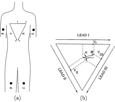
2.1 Special conductive regions and pacemaker ( SA node) of the heart. 3 2.2 A normal electrocardiogram ... 4 2.3 A sketch of the dipole field of the h e a r t ... 5 2.4 (a) Placement of electrodes for standard leads, (b) The

Einthoven triangle. Employment of heart vector and lead vec­

tors to find lead voltages. 7

2.5 (a) Positions of the precordial leads on the chest wall (b) Con­ nection of electrodes to the body to obtain Wilson’s central

terminal. 7

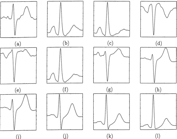
2.6 Typical ECG waveforms of (a) D1 (b) D2 (c) D3 (d) aVR (e) aVL (f) aVF (g) VI (h) V2 (i) V3 (j) V4 (k) V5 (1) V 6 ... 8

3.1 General form of the nonrecursive adaptive filter...11 3.2 Original and reconstructed signals of V6 using (a) 7 leads (b) 6

leads (c) 5 leads.

3.3 Original and reconstructed signals of V6 using leads with com­ binations (a) D2, VI, V2, V3, V4 (b) Dl, D2, VI, V2, V3

13

14

4.1 Special conductive regions and pacemaker ( SA node) of the heart. 16 4.2 The QRS Detector m o d u le ...16 4.3 Commonly used Fiducial M a rk e rs ... 17

5.1 Block diagram of the method proposed... 23 5.2 (a) ECG leads with EMG noise (b) output of SVD... 24 5.3 (a) ECG leads with baseline wander (b) output of SVD... 24 5.4 Plots of power calculated employing two and three SVD chan­

nels intwo different morphologies with (a) 7.9% (b) 0.5% per­ centage error between them ... 28 5.5 Typical TPS t y p e s ... 28 5.6 Strip chart of one QRS complex showing (a) First channel of

SVD output (b) second channel of SVD output (c) TPS em­ ploying the first two channels (d) absolute value of derivative of T PS... 30 5.7 Derivatives of typical T P S ’s plotted in Fig. 5 .5 ... 30

5.8 Sub-blocks of search algorithm. 31

5.9 Plot of RR intervals versus QRS duration...33

6.1 Performance m atrix...35 6.2 The plots for patient (a) 410 (b) 411 (c) 412 (d) 692. 36 6.3 The plots for patient (a) 695 (b) 696 (c) 697 (d) 698 (e) 705 (f)

708 (g) 710 (h) 714 (i) 719 (j) 720 (k) 721 (1) 722... 37 6.4 The plots for patient (a) 726 (b) 728 (c) 729 (d) 730 (e) 731 (f)

733. 38

6.5 Histogram of difference between QRS complex duration pairs

obtained employing both methods. 40

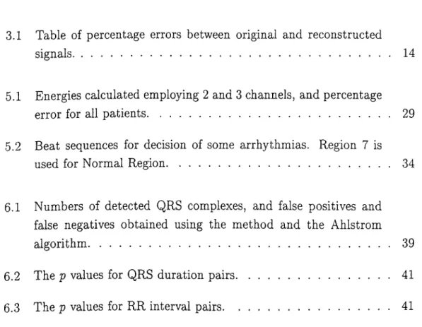
LIST OF TABLES

3.1 Table of percentage errors between original and reconstructed signals...14

5.1 Energies calculated employing 2 and 3 channels, and percentage error for all patients... 29 5.2 Beat sequences for decision of some arrhythmias. Region 7 is

used for Normal Region...34

6.1 Numbers of detected QRS complexes, and false positives and false negatives obtained using the method and the Ahlstrom algorithm... 39 6.2 The p values for QRS duration pairs... 41 6.3 The p values for RR interval pairs... 41

C hapter 1

In trod u ction

Ever since Einthoven introduced electrocardiography as a new method to di­ agnose heart disease [1], its use and importance has expanded. The electro­ cardiogram (ECG) is a non-invasive technique. It is inexpensive, simple.

Fisch mentioned [2] th at the ECG

1. still serves as an independent marker of myocardial infarction 2. reflects anatomic, metabolic alterations

3. demonstrates a variety of complex electrophysiologic concepts through deductive reasoning

4. is a stimulus for a laboratory conflrmation of postulated mechanisms and concepts

5. is vital for proper diagnosis and therapy

6. is without peer for the diagnosis of arrhythmia.

Although the sixth item involves the diagnosis of arrhythmia, most of the arrhythmia types can not be seen on rest electrocardiogram due to short span of time. Instead Holter [3] or exercise ECG methods are used in diagnosis of arrhythmia. The first paper regarding the exercise test was published by Master [4] in 1929.

The exercise ECG test (stress ECG test) is another important and non- invasive diagnostic tests in clinical evaluation of patients with suspected or

known cardiovascular disease. The exercise ECG test is also a very useful tool as a screening procedure for healthy individuals who are considered to be at possible risk of heart disease.

The exercise ECG test is performed by a motor driven treadmill in most medical institutions in the United states of America. However, in European countries, the treadmill exercise ECG test is less popular. Instead a bicycle ergometer is commonly used. At present, various multistage exercise protocols have been developed by different investigators for the exercise ECG test using either a motor driven treadmill or an electrically braked bicycle ergometer [5].

The exercise ECG test requires 15 to 30 minutes record with at least 2 channels. On the other hand one channel is recorded throughout 24 hour in Holter test. In all of the conventional methods of arrhythmia analysis tools at most two channel information is used. In the method proposed in this thesis, 12 lead ECG information is composed into two orthogonal channels. This method implemented is applied to 22 patients’ data. The data

• is obtained using a 12 bit D /A converter • have sampling rate of 500 samples/second • is recorded through 8 channels

• have lengths between 9.5 to 26.5 minutes.

In Chapter 2 general elecrophysiology of the heart is described. Chapter 3 presents, compares and comments about two methods for reconstruction of a lost ECG channel. The general concepts about arrhythmia and QRS detection, some QRS detection algorithms in the literature are explained in Chapter 4. The method proposed in this thesis is described in Chapter 5. The algorithm suggested in [6] is implemented for comparison purpose. Results and comparisons of the two algorithms are provided in Chapter 6. Finally, conclusions are given in Chapter 7.

C hapter 2

T h e E lecrophysiology o f T he

H eart

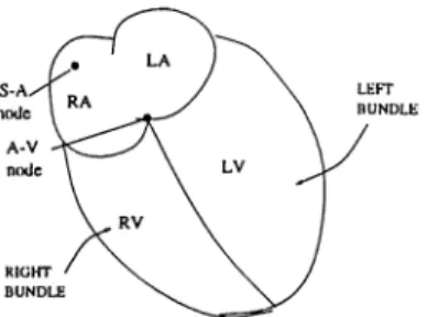
Heart is a unique organ which produces it’s own electrical stimulation. The major elements of the electrical structure of the heart are the working muscle of the atria and ventricles, the specialized conduction tissue, and the pacemaker cells [7]. The general anatomical structure is shown in Fig. 2.1

Figure 2.1: Special conductive regions and pacemaker ( SA node) of the heart. The pacemaker cells, found at the SA node are self-excitatory. T hat is, instead of maintaining constant resting potential, a regular succession of action potential, elicited when an adequate stimulating current is passed thorough a cell, originates. These action potentials lead to a series of heart beats.

Action potentials initiated from SA node, excites the neighboring cells. A cell to cell excitation takes place in the atria. When this excitation reaches to AV node, specialized conduction cells take the impulse to ventricles. Since there is non-conducting tissue between atria and ventricles. The conduction cells conduct the excitation slowly. Hence a latency is introduced between

atrial and ventricular excitation [7].

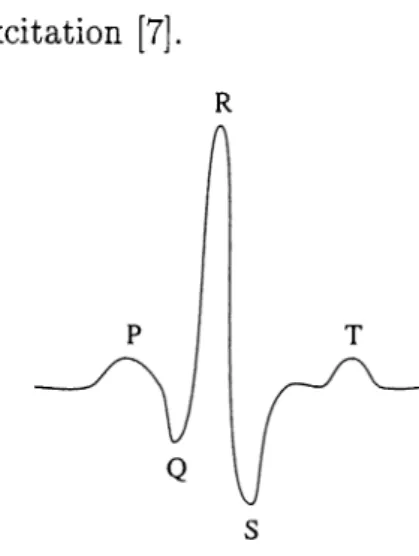
R

Figure 2.2; A normal electrocardiogram

As the cardiac impulse passes through heart at every cardiac cycle, elec­ trical currents spread into the tissues surrounding the heart, and a projection of these currents appear on the surface of the body. This phenomenon can be used as a diagnostic tool for examining some of the functions of the heart by placing electrodes on the surface of the body. Then electrical potentials gener­ ated by these currents can be recorded which is known as the electrocardiogram. A normal electrocardiogram is shown in Fig. 2.2.

2.1

H eart Vector (D ipole)

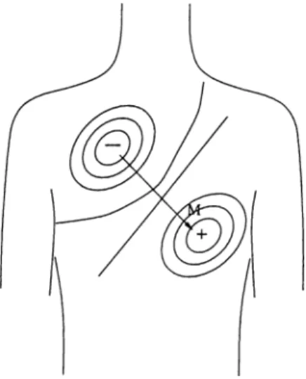
At any instant of time during activation of the heart, the source is distributed to all the surface of the heart. This activity can be approximately represented as a vector quantity. A simple model have been developed to represent this activity. In this model the heart consists of an electric dipole located in the thorax. It can be represented by its dipole moment. This is a vector directed from negative charge to the positive charge. In elecrophysiology, this dipole moment is known as heart vector (dipole), and is represented by H, as shown in Fig. 2.3 [8]. The heart dipole is expected to vary both in magnitude and in direction in a smooth manner. The heart vector is related to volume dipole moment density, Jj, of the heart by

or

H = J JidV

= I j i d v , Hy = I j ; d v , H , = I Ji dV

(2.1)

Figure 2.3: A sketch of the dipole field of the heart

where H is the heart vector ( a function of time), and Ji = J 'a x + Jj)ay + J'a.z More details are given in [7] and [8].

2.2

Lead Vector

The voltage measured between two body surface electrodes depends on the lead location, heart location, heart vector and torso volume inhomogeneities. For a particular heart vector location and lead position a unit magnitude heart vector can be written as

H — h^jUx T h y 3 .y T h ^ ^ Z ' The lead voltage Vi is given by

Vi — h x lx T hjl*

(2.3)

(2.4) where li represents lead voltage formed by component of H, if it had unit length x ,y , or z components. Eqn.( 2.4) can be written as a dot product; th at is

Vi = H · 1. (2.5)

This expression demonstrates the lead voltage dependence on the heart vector and lead vector which reflects the geometry and conductivity [7].

2.3

Standard Leads

The standard leads, first introduced by Einthoven [8] and [1], were placed at wrists and ankles. Placement of electrodes on extremities is not very critical since extremities are isopotential. The right leg is grounded for noise cancela­ tion purposes (Fig. 2.4 (a)). Then the three lead voltages are

Vi = ^LA — ^ñ.4 (2.6)

Vll = ^LL — (2.7)

VlII = ^LL — ^LA (2.8)

A typical lead voltage waveform is in Fig. 2.2. The P-wave is caused by electrical potentials generated as the atria depolarize prior to contraction. The QRS complex is caused by potentials generated when the ventricles depolarize prior to contraction. Therefore both P and QRS complex are depolarization waves.

The T wave is caused by potentials generated as the ventricles recover from the state of depolarization. This process occurs in ventricular muscle 0.25 to 0.35 second after depolarization, and this wave is known as a repolarization wave. There is another repolarization wave caused by electrical potentials as the atria repolarized. But this occurs in 0.15 to 0.25 second after the P wave. However, this occurs at the same time th at the QRS wave is being formed. Therefore, the atrial repolarization wave, known as the atrial T wave, is usually totally obscured by the much larger QRS wave. For this reason, an atrial T wave is rarely observed in the electrocardiogram [9].

By means of Kirchoff’s law the net potential drop around a closed loop is zero, then

i^LA ~ ^Ra) + i^RA — ^ Ll) + i^LL ~ ^La) = 0. (2-9) Using Equations (2.6)-(2.8), Eqn.(2.9) can be written as

+ Vjij = Vji (2.10)

so th at only two limb lead voltages are independent. According to Eqn.(2.5) the lead voltages are found by projecting the heart vector on the perspective lead vector. This is illustrated in Fig. 2.4 (b).

Additional electrocardiographic data are obtained from leads placed on the chest (precardium) (Fig. 2.5 (a)). Each precordial lead is measured against the Wilson central terminal (CT) as a reference. The CT is formed at the junction

LEAD I

Figure 2.4: (a) Placement of electrodes for standard leads, (b) The Einthoven triangle. Employment of heart vector and lead vectors to find lead voltages.

of three 5K resistors the other end of each being connected to a different limb lead as illustrated in Fig. 2.5 (b). Assuming the use of a very high input impedance potential measuring system, $ c r gives

^CT = 'i’ÄA + ^LA + ^LL (2.11)

(a)

Figure 2.5: (a) Positions of the precordial leads on the chest wall (b) Connec­ tion of electrodes to the body to obtain Wilson’s central terminal.

In addition to standard leads and precordial leads, there are three more leads called augmented leads, aVR, aVL, and aVF. These leads are for diag­ nostic purposes. Augmented leads are calculated, employing standard leads as

follows: qV R aVL &VF D1 + D2 D 1 - D 3 2 D2 + D3 (2.12) (2.13) (2.14)

Typical shapes of every lead is in Fig. 2.6. The augmented leads and D3 are not measured. They are calculated using D1 and D2.

(a)

(c)

(1)

Figure 2.6: Typical ECG waveforms of (a) D1 (b) D2 (c) D3 (d) aVR (e) aVL (f) aVF (g) VI (h) V2 (i) V3 (j) V4 (k) V5 (1) V6

C hapter 3

R econ stru ction o f A Lost ECG

C hannel

A patient under stress test, walks or runs on a treadmill. This test takes a period of between 10 to 30 minutes. During the test, some channels may be lost due to non-conducting electrodes. A method based on least squares was suggested by M ortara to recover the signal in channels [10]. The least squares method minimizes mean squared- error between the original signal and the estimated signal. That is

M S E = < { x - y f > (3.1)

where x and y are the vectors with entries original and reconstructed channels respectively. The operator < > shows mean. The vector y can be calculated as

y(z) = C x(i) (3.2)

where C is the coefficient matrix involving the coefficients for reconstructing all channels individually. For simplicity let us derive the formulation for one channel reconstruction and obtain a coefficient vector, Cj. This vector is used to form the whole C matrix. If Xj is the lost channel let us denote xy as the vector with the remaining seven channels as its entries:

X j =

iT

Xi Xj —\ Xi (3.3)

The mean-squared error is < {xj minimizes this equation is

c j x , y

Cj = < x j x j > ^ X j X j .

>. Coefficient vector Cy which

Using 3.4 whole C matrix can be formed performing the following multiplica­ tion. Diagonal entries of C matrix must be fixed to zero.

- I - 1 < Xl,Xl > < Xi , X2> . . .< Xi,Xs > < X2,Xl > < X2, X2 > . . . < X-2,Xs > < X S , X l > < Xs , X2 > . . ■< X8, x& > 0 < Xi,X2 > . . .< Xi,X^ > <X2,Xi > 0 . . . <X2, X&> < Xs,Xl > < Xs,X2 > ■ ■ ■ 0

In this method C matrix is calculated once and used within all data re­ laying on the assumption that EGG pattern does not change in time. But in exercise EGG shape of QRS complexes may change in time. Also frequency of QRS pulses varies in time due to changing performance of patient. As a result least squares is not an appropriate method for reconstruction of a lost channel in exercise EGG. In order to investigate possible improvements in the reconstruction of the lost channel or channels, an adaptive approach is used. The output of the adaptive filter is compared with the output of least squares.

3.1

L M S-N ew ton Algorithm

Before going into the details of LMS-Newton algorithm, a short review about adaptive filtering will be given.

3.1.1 A daptive Filtering

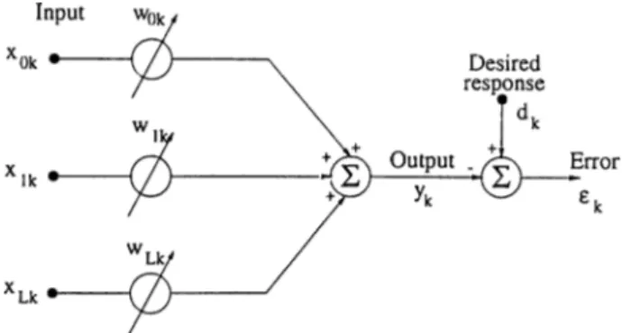
A nonrecursive adaptive filter is fundamental to adaptive signal processing. A diagram of the general form of the nonrecursive adaptive filter is shown in Fig. 3.1.

The main purpose of the adaptive filtering is minimization of a cost function of error, €. This error is the difference between a desired signal, dk, and output of adaptive filter, yk- The coefficients, w, varies adaptively.

efc = dk - Vk = d k - X j W = dk - W ^ X , The most common cost function is the mean-square.

4 = 4 + w ^ X k X l w - 2 d k X l w 10

(3.5)

Figure 3.1: General form of the nonrecursive adaptive filter.

e

{

4

]

=

4

\ +

wf£[XtXf|w - 2£;|4xaw

The mean-square-error function can be more compantly expressed as fol­ lows. Let R be defined as R = E[X.j^X.^] and similarly P as P = £'[di,X)3], then mean-square error in Eqn.(3.7), which is designated by can be re-expressed as

M S E = e = E[el] = E[dl] -b W ^R W - 2 P ^ W (3.8)

The mean-square error is a quadratic function of the components of the weight vector when desired response and input vector are stationary stochas­ tic variables. A concave quadratic function has always a minimum. Many adaptive processes employ gradient search techniques to seek the minimum. Gradient of designated as, V((^) can be obtained by differentiating expression in Eqn.(3.8)

A

V

d W = 2RW - 2P (3.9)

To obtain the minimum mean-square error (MMSE), a W is calculated setting gradient to zero, leading to

W *R "^P (3.10)

where W* is the optimal value of W .

3.1.2

Gradient Search by N ew to n ’s M ethod

A recursive method can be established to search the minimum of the mean square cost function. Multiplying both sides of Eqn.(3.9) by j R “ ^ and substi­ tuting into Eqn.(3.10), we get

) (3.11)

11

w * = W - - R " V

Changing this result into an adaptive form

W ,+ i = Wfc - /rR -V ,- _(3.12)

Using a noisy gradient estimate V, in place of V and ej. as an estimate for (Eqn.(3.6))

Vt = -2ekXk (3.13)

Substituting Eqn.(3.13) into Eqn.(3.12) the adaptive LMS-Newton Algorithm’s coefficient adaptation can be found as

W,.+i = W , + 2/rR-i£,Xfc _(3.14)

Since real R ^ is not known an estimate, R for that is used. An update for th at is as follows [11]:

r»-l -

1

- O i----;--- --- )

1 - O' ^ ^ 1 - Q! + ax^’RfciiXt

where and a are constants between zero and one. But for convergence

1

0 < H <

(3.15)

^max

where Xmax is the maximum eigenvalue of the input correlation matrix, R.

3.1.3

R esults

All channels are reconstructed using the remaining seven leads for 22 exercise ECG data. Also, the effect of two and three lost channels is examined. All the remaining six and five leads the combinations are employed. Effect of increasing lost channels is observed.

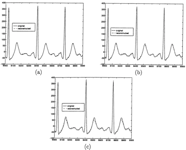
When the number of lost channels is increased, error between original and reconstructed signals are increased. This phenomenon can be observed in Fig. 3.2. In Fig. 3.2 (a) seven channel reconstruction of V6 is shown. Percent­ age error between original and reconstructed signal is 3.6%. In Fig. 3.2 (b) plot of reconstructed signal using six channels (D l, VI, V2, V3, V4, V5). The percentage error is 7.4%. In Fig. 3.2 (c) sketch of original signal and recon­ structed signal using 5 leads (Dl, V2, V3, V4, V5) of V6 is shown. It has a percentage error of 9.3%.

The correlation coefficients between every pair of channels differs. The observations on data from 22 patients show that, D2 is less correlated to other

(c)

Figure 3.2: Original and reconstructed signals of V6 using (a) 7 leads (b) 6 leads (c) 5 leads.

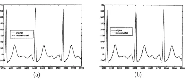
channels, since there is no other lead with the same direction. Since it involves a big amount of energy of EGG, when it is lost it can not be reconstructed properly. Also different results are obtained for different configurations of input channels. In Fig. 3.3, two reconstructed signals for V6 employing different combinations of input channels.

In Table 3.1, percentage errors between original signals and reconstructed signals obtained using one record can be seen. Different results are recorded when six and five leads combinations are used.

3.1.4

Problem s w ith this M ethod

There are some problems with this method.

• Since the aim is to reconstruct the lost channel, the adaptive filter is less instrumental, because the desired signal is also the lost channel. The coefficients obtained just before loss of the channel may be stored. Then these coefficients are employed to reconstruct the lost channel.

(a) _(b)

Figure 3.3: Original and reconstructed signals of V6 using leads with combi­ nations (a) D2, VI, V2, V3, V4 (b) D l, D2, VI, V2, V3

# of i/p channels 7 6 5 Ghannel % Error min % Error max % Error min % Error max % Error D l 9.4 9.5 23.2 10.8 24.8 D2 16.6 13.9 21.8 17.4 33.9 VI 11.9 11.5 30.6 15.0 30.6 V2 2.6 2.6 6.1 3.0 20.6 V3 2.4 2.4 3.5 2.6 22.4 V4 2.4 2.5 5.6 2.8 12.3 V5 4.1 3.3 7.8 3.2 10.55 V6 3.6 3.5 7.4 3.9 11.4

Table 3.1: Table of percentage errors between original and reconstructed sig­ nals.

• High correlation between EGG channels makes the input correlation ma­ trix ill conditioned. This causes error between original and estimated signals. Instead of using original EGG signals for reconstruction, or- thogonalized EGG signals are used [12]. This process also reduces the dimension of signal space.

C hapter 4

A rrh yth m ia

4.1

W hat is Arrhythm ia ?

Cardiac Arrhythmia are associated with electrical instability and, hence, with abnormal mechanical activity of the heart. They can and do interfere with the normal circulation of oxygenated blood around the body. Some arrhythmia can halt this flow and can be fatal. In many cases, arrhythmia can be treated with drugs or electric shock to control and or to stop them. Detection of arrhythmia is one of critical problems in cardiac electrophysiology.

A cardiac cycle normally originates in the sinus node which is high in the right atrium. If a depolarization wave originates in a site other than the sinus node, an arrhythmia results. There are several mechanisms th at can be re­ sponsible for arrhythmia. In clinical practice, arrhythmia are often subdivided according to their site of origin. When it is known that the source of the ar­ rhythmia lies in the atria and not in the sinus node (Fig. 4.1), the arrhythmia is called atrial. The QRS shape of an atrial complex is usually similar to that of the sinus complex except that it appears prematurely and has a differently shaped P-wave. If the source of an arrhythmia is in the atria or close to the A-V node, the resulting arrhythmia is called supraventricular (atrial arrhyth­ mia are a subgroup of supraventricular arrhythmia). If the source is in the ventricles, it is called ventricular. Ventricular complexes tend to have broader QRS complexes than sinus complexes because of asynchronous activation of the bundle branches.

Figure 4.1: Special conductive regions and pacemaker ( SA node) of the heart.

There are variety of terms used to describe an abnormal ventricular com­ plex. The most common are: ventricular ectopic complex (VEC), ventricular ectopic beat (VEB), premature ventricular complex (PVC), ventricular pre­ mature beat (VPB), and ventricular premature deflection (VPD). Although the terms may appear to distinguish different types of ventricular complexes, they are generally used synonymously.

4.2

QRS D etection

QRS detection ( Fig 4.2) is the first analysis stage in which pattern recognition is important. The QRS detector is the most important part of an arrhythmia monitor, since the accuracy of the whole system depends on it.

ECG SIGNAL

Figure 4.2: The QRS Detector module

The QRS detector can be divided into two parts: an initial analysis stage that detects the presence of a QRS and a subsequent stage that performs a timing marker or fiducial point for detected QRS complexes. The search process for QRS complexes requires that candidate waveforms meet two or more criteria.

The most general QRS criterion is that the waveform has a certain mini­ mum amplitude, the purpose of which is to eliminate to a first approximation the false detection of P-waves, T-waves, and low-to-medium level noise. This amplitude threshold may be fixed or may vary depending on the height of the previously detected complexes. After a candidate waveform has passed the

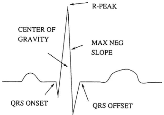
Figure 4.3: Commonly used Fiducial Markers

amplitude criterion, it must then meet certain criteria regarding shape. These shape criteria pertain specifically to the characteristics of the slopes that com­ prise the waveform. Once a candidate waveform has qualified for being a QRS complex, the timing of the event must be established. This information, which must be reliable, is passed to subsequent analysis stages for use in the com­ putation of beat characteristics, RR intervals, prematurity, QRS width, etc. Some of the commonly used fiducial markers are illustrated in Fig. 4.3.

4.3

Some Commonly U sed QRS D etection

A lgorithm Types

In this section, some of the QRS detection schemes will be described. A large number of QRS detection algorithms are explained in the literature [6,13-20]. All of these schemes employs one original EGG lead signal information. Their performances are compared in [21].

Algorithm 1

This algorithm was derived by Moriet and Mahoudeaux [15]. In this scheme an amplitude threshold is calculated as a fraction of largest positive valued element of original signal x. Then first derivative y is calculated at each point of X such th at

y{n) = x(n + 1) — x{n — 1)

A QRS candidate occurs when three consecutive points in the first derivative array exceed a positive slope threshold are are followed within the next 100 ms by two consecutive points which exceed the negative threshold. All data points in the ECG between the onset and offset must meet or exceed the amplitude threshold.

Algorithm 2

This algorithm is first developed by Fraden and Neuman [16]. A threshold is calculated as a fraction of the peak value of the ECG signal x. Then the raw data is rectified, yo = l^^l, the rectified signal is passed through a low level clipper such that

yi(^) =

?/o(n) if Vain) > amplitude threshold 0 if yi){n) < amplitude threshold

The first derivative is calculated at each point of the clipped, rectified array:

2/2(n) = y\{n + 1) - 2/1 (n - 1)

A QRS candidate occurs when a point in y-iiji) exceeds a fixed constant thresh­ old.

Algorithm 3

This algorithm was developed by Menard [17]. The first derivative is calcu­ lated for each point of the ECG, using the formula

y{n) = - 2 x ( n - 2) - x{n - 1) + x{n + 1) + 2x{n + 2)

The slope threshold is calculated as a fraction of the maximum slope for the first derivative array. The first derivative array is searched for points which exceed the slope threshold. The first point above the threshold is taken as an onset of a QRS candidate.

This algorithm was first suggested by Baida [18]. The absolute value of the first and second derivative are calculated from the ECG:

7/o(n) = \x{n + 1) - x{n - 1)1

y\{n) = \x(n + 2) - 2x{n) + x{n - 2)\ These two arrays are scaled and then summed;

2/2(n) = 1.3yo{n) + l.lj/i(n )|

This array is scanned until a threshold is met or exceeded. Once this occurs, the next eight points are compared with respect to the threshold. If six or more of these points meet or exceed the threshold, the criteria for identification of a QRS candidate is met.

Algorithm 5

This algorithm is taken from Ahlstrom and Tompkins [6]. The rectified first derivative is calculated from the ECG:

^o(n) = |a:(n + 1) - x{n - 1)| This signal is then smoothed:

yi{n) = [yo(n - 1) + 2yo{n) + yo{n + l)]/4 The rectified second derivative is calculated:

|/2(n) = \x{n + 2) - 2x{n) + x{n - 2)1

The rectified, smoothed first derivative is added to the rectified second deriva­ tive, yz = yi + y2- The maximum value of this array is determined and scaled to serve as primary and secondary thresholds, yz is scanned until a point ex­ ceeds the primary threshold. In order to be classified as a QRS candidate, the next six consecutive points must all meet or exceed the secondary threshold.

Algorithm 6

A lgorith m 4

This algorithm was developed by Engelse and Zeelenberg [19]. The ECG is passed through a differentiator with a 62.5 Hz notch filter.

yo{n) - x(n) - x{n - 4) 19

This d ata is then passed through a low-pass filter.

y\{n) = yo(n) + Ayo{n - 1) + 6yo{n - 2 ) + Ayo{n - 3) + yo(n - 4)

Two thresholds are used, equal in magnitude but opposite in polarity. The output of the low-pass filter is scanned until a point with amplitude greater than the positive threshold is reached. This point is the onset of a 160 ms search region. Let yi{i) > threshold If no other threshold crossings occur within the 160 ms search region starting from onset, the occurrence is classified as baseline shift. Otherwise, the following three conditions are tested:

Condition 1: If y\{i + j) < —threshold 0 < j < 160ms Condition 2: If y\{i + j) < —threshold 0 < j < 160ms

and

yi{i + k) > threshold j < k < 160ms Condition 3: If yi(i + j) < —threshold 0 < j < 160ms

and

yi(i + k) > threshold j < k < 160ms and

yi{i + 1) < —threshold k < I < 160ms

If any of the above conditions apply, the occurrence is classified as a QRS candidate.

Algorithm 7

This algorithm is taken from Okada [20]. The first stage smoothes the ECG using a three-point moving average filter:

yo{n) = [x{n - 1) + 2x(n) + x{n -\-1)1/4

The output of the moving point averaging filter is passed through a low-pass filter/

i n+m

The difference between the input and output of the low-pass filter is squared, y-2 = (t/o — yiY - The squared diffe.rence is filtered:

n + m

y3{n)=y2{n){

k = n — m

A fourth array is formed using the following formula:

yz{n) if [yo(n) - yo{n - m)][i/o(n) - yQ{n + m)] > 0 2/4 (n) =

0 otherwise

The maximum value of this array is determined and scaled to form the thresh­ old. A QRS candidate occurs when a point in 2/4 exceeds the threshold.

Algorithm 8

This algorithm is suggested by Pan and Tompkins [13]. First ECG signal is passed through a band-pass filter composed of cascaded low-pass and high pass filters for noise rejection.

2/o(n) = 2yo{n - 1) - yo{n - 2) -t- x{n) - 2x{n - 6) -b x{n - 12) (LPF) yi{n) = 2/o(n) + 322/o(n - 16) - 2/o(n - 32) - y,{n - 1) (HPF) The band-pass filtered signal is differentiated employing a five-point derivative with th e difference equation

2/2(^) = g [~2/i(^ — 2) — 2 y i ( n — 1) -b 2 y i { n -b 1) -b 2/1(7^ + 2)]

After differentiation, the signal is squared, 2/3 = [У2]^· Then moving window integration is applied to the squared signal,

2/4(71) = ^[2/3(71 - N + . l ) + y ^ { n - A -b 2) + ... + 2/3(77)]

Two thresholds are calculated, one from the integrated signal, 2/4, the other from filtered signal, 2/2· To be identified as a QRS complex, a peak must be recognized as such a complex in both the integration and band-pass filtered waveforms.

Algorithm 9

This algorithm is proposed by Akazawa [14]. First a digital filtering is executed

1 Wf

2/0(77) ^ h{\k\)x{n + k)

Second, moving average is applied

2/1(77) = E 12/0(77 + A:)] ^yyj + i

Then a logarithmic transformation is exploited to this filtered and averaged signal.

y^in) = int[M \og[l + 2/1 (n)}]

Decision of the threshold for 2/2 (n) is a key to detection of QRS. A time varying threshold T{n) is decides as follows. First histogram for the amplitude of 2/2, denoted by D (n, k) is given by

Wh

1 if 2/2(n + 2) = A; 0 otherwise

Second, the distribution function, H (n,p), is obtained by integrating the his­ togram. When H {n,p) is equal to a time varying constant K ff, the value p is taken as the threshold T(n). 2/2 and T(n) are waveforms intersecting at onset and offset points of QRS complexes and T waves. To distinguish QRS complexes from T waves following criterion is employed

D(n, k) where u{n, i, k) _{= {}f 1 0 offset s = E {2/2(0 i=onset T(i)) > St

4.4

Arrhythm ia D etection and Classification

As described in the previous section arrhythmia analysis module is a subse­ quent section of the QRS detector. They are designed to detect only some of the more obvious abnormal rhythms such as ventricular salvos, bigeminy, trigeminy, tachycardias, and bradicardias. Arrhythmia detection and classi­ fication can be accomplished using RR intervals and QRS durations. QRS duration is not needed in detection of some arrhythmia. For example, R on T beats, APB, Paroxismal bradycardia, etc. In detection of these type of ar­ rhythmia, RR intervals of three or more consecutive beats are used. In general, every RR interval is compared with an average RR interval. Hence irregular rhythms are detected.

On the other hand, in addition to RR interval QRS duration must be employed in detection of some of other arrhythmia types. For example, PVC’s and couplets. Similar to detection of irregular rhythms, duration of every QRS complex is compared with an average QRS duration.

C hapter 5

M eth od

In this chapter, a method for detecting and analyzing the arrhythmia will be proposed. The block diagram of the stages involved are depicted in Fig. 5.1. A first stage process is orthogonalization of 8 lead data. The aim is to decrease the number of channels. The second step is calculating the power signal. The purpose is to obtain a single signal representing all the ECG signal. In order to find the onset and offset points, a third stage, differentiation introduced. The last part of the QRS detection algorithm is the search stage. An analysis phase is added to obtain a full package of arrhythmia analysis tool. Every step will be discussed individually in this chapter.

Figure 5.1: Block diagram of the method proposed.

5.1

O rthogonalization of ECG Signal using

SVD

This is the first stage of the algorithm. 8 lead ECG signal is reduced into three orthogonal channels using singular value decomposition. The orthogonaliza­ tion process maintains th at the first three channels are free from noise. Noise

is accumulated to the other channels. Two major noise sources exist in ECG. One of them is muscles around the electrodes. Noise sourced from muscles is called EMG noise. Frequency range of EMG noise is a bit larger than ECG and overlaps with it. Effect of SVD to an ECG with EMG noise is shown in Fig. 5.2. D1 and D2 are highly corrupted with EMG noise. First two channels of output of SVD does not involve EMG noise so much. Another noise source is the respiration of patient. This is a low frequency noise ( below 0.5 Hz) and is called baseline wander. Input and output of SVD when ECG is corrupted with baseline wander can be seen in Fig. 5.3. D1 involves baseline wander. After processing employing SVD, noise is accumulated in channel 4 and first two channels are noise free. Also sometimes one or more ECG channels may be lost due to non-conducting electrodes. When this kind of a situation occured, the method used the remaining ECG channels to form the SVD outputs.

(a) (b)

Figure 5.2: (a) ECG leads with EMG noise (b) output of SVD.

2

(a)

CH7 CH0

(b)

Figure 5.3: (a) ECG leads with baseline wander (b) output of SVD.

5.1.1

SVD

Let A G ra n k(A ) = r. Then there exist orthogonal matrices U G T^mxm and V G such that

A = U S V ^ (5.1) where S = and S = diag{a\, S 0 0 0

., cTr) with cTi > ... > (Tr > 0 and

U ^ U - Ixn, V ^ v = In

P ro o f: See [22].

The numbers a \ , . . . , a r together with (Jr+i = 0, ...,cr,i = 0 are called singular values of A. Eqn.(5.1) can also be written as sum of a r rank 1 matrices.

r

A = ^(T,UiV?’ (5.2)

»■=1

The columns of U, Uj, are called the left singular vectors of A while the columns of V, Vi are called right singular vectors of A. The rank 1 matrices in Eqn.(5.4) and singular vectors are unique if all singular values are distinct [23].

5.1.2

Som e Useful Properties of SVD

Each left singular vector, Ui represents a filter in space such as UjA = aivi

Also output signal of this filter reaches a maximal rms value for Uj is orthogonal to all previous left singular vectors:

Vx G j — l , . . . , i — l

< IIA ^u ill = a. (5.3)

Another important property of the SVD is its relation to the eigenvalue decomposition of the nonnegative definite symmetric matrix A A ^, given by

A A ^ = (5.4)

5.1.3

Online Algorithm

Measurement signals can be written as a linear combination of source signals, plus noise [23]

m (t) = T s(t) + n (t) (5.5) where m (t) is measurement vector, T is transfer vector, s(t) is the source signals and n (t) is noise vector. For time invariant case Eqn.(5.5) can be written as

M = TS + N (5.6)

For p electrode signal, r source signals and q samples, M, N G S G and T G Then M M ^ is given by Eqn.(5.4). Assuming noise signals are time orthogonal to each other and p then

= alrlp Then using Eqn.(5.6) and Eqn.(5.7)

2rr'^ , _2

MM' = T S |T +

(5.7)

(5.8)

where = SS^. If transfer matrix, T is diagonalized employing a diagonal- ization method, mainly Given’s Rotation Method [24] then

0 = Q?T (5.9)

Therefore Eqn.(5.8) becomes

M M ^ = Q Te sie Q T^^ + <T.5,ip = Q (D + (7^Ip)Q’· (5.10) (5.11) in which D = 0S§© 0 0 0 (5.12) 26

and Q is an orthonormal p x p matrix constructed by adding an orthonormal set of vectors spanning the orthonormal complement of the column space of Qt· If the SVD of M is written as M = _{U i U2} E l 0 0 S2 Vi^ V2' (5.13)

with U i E l Since the columns of U i span the same invariant subspace of M M ^ as the columns of Q x, U iU i^ = QtQt^. Moreover if the

first r eigenvalues of M M ^ are disjoint, the first r left singular vectors of M are equal to the unit vectors in the direction of the respective transfer vectors. Therefore, Uj represents a filter in space for which output signal contains a contribution proportional to the ¿th source signal, corrupted by noise. So source vector can be estimated by

S = UiM = 0 S + u Jn (5.14)

An online method was suggested to solve the problem in Eqn.(5.14) in [23]. Since exact U is not known, it is estimated. The algorithm is;

a) U o := 1, Co = 0. b) for i = 1 to g

1. s(t,·) =

2. Bi = a ^ C i.i + s{U )s{tif 3. C, = Qi^BiQ i

4. Ui = U i_iQ i

where O' is a forgetting factor and

Ci = UfMiMi^Ui

5.2

Calculation of Total Power Signal

As described in the previous section, 12 lead ECG signal is reduced into three orthogonal channels. The energy content of third channel changes from patient to patient. It has either very low power with respect to other two or only noise.

Figure 5.4: Plots of power calculated employing two and three SVD channels intwo different morphologies with (a) 7.9% (b) 0.5% percentage error between them.

Making use of the orthogonality of these new channels, Total Power Signal (TPS) is calculated by summing the squares of first two channels (Fig. 5.6 (c)).

Employment of these channels in TPS yields approximately 92% to 99% of ECG power contained in all channels (Table 5.1). Power waveforms for patients 696 and 705 are plotted in Fig. 5.4. This patient are chosen because of error for 696 is maximum and 705 is minimum. In the worst case (Fig. 5.4 (a)), although error between two power signals is 8%, shape of signal is not effected. Hence employing two channels instead of three channels is a good approximation.

Also shape of the TPS is an important point in the detection of QRS complexes. There are two main types of T PS’s (Fig. 5.5). These types are classified from the data of 22 patients. Most of the T PS’s are similar to skecth in Fig. 5.5 (a). There is a main lobe in TPS. This type of a signal is very appropriate for detection of onset and offset points. Some of the T PS’s are in the form as in Fig. 5.5 (b). There are two main lobes in TPS. This must be considered in detection algorithm.

(a) (b)

Figure 5.5: Typical TPS types

Patient # Energy of TPS (2 Channels) xlE· -t- 9 Energy of TPS (3 Channels) x i f; + 9 Percentage Error 410 0.5294 0.5503 3.8 411 1.1081 1.1152 0.6 412 1.2455 1.2528 0.6 692 0.3154 0.3190 1.1 695 0.5797 0.5865 1.1 696 0.1846 0.2006 7.9 697 4.3901 4.4304 0.9 698 0.4615 0.4711 2.0 705 1.4003 1.4074 0.5 708 0.6551 0.6756 3.0 710 0.4670 0.4847 3.6 714 0.5983 0.6066 1.4 719 1.0862 1.0928 0.6 720 0.9307 0.9647 3.5 721 0.3874 0.3981 2.7 722 0.7557 0.7752 2.5 726 0.4296 0.4520 5.0 728 0.6210 0.6263 0.8 729 0.1902 0.1931 1.4 730 0.3607 0.3777 4.5 731 0.5734 0.5780 0.8 733 1.3341 1.4170 5.8

Table 5.1: Energies calculated employing 2 and 3 channels, and percentage error for all patients.

5.3

DifFerentiation

QRS complex contains higher frequency components than the other waves in ECG. Hence the signal is differentiated to provide the QRS complex slope in­ formation. Absolute value of two-point derivative with the difference equation

y{n) = \x{n + 1) — x{n — 1)1 is exploited.

The detection of onset and offset of QRS complex is easier using the output of differentiator Fig. 5.6 (d) than the input of the differentiator Fig. 5.6 (c). The plots of derivatives of typical TPS signals in Fig. 5.5 are given in Fig. 5.7.

Figure 5.6: Strip chart of one QRS complex showing (a) First channel of SVD output (b) second channel of SVD output (c) TPS employing the first two channels (d) absolute value of derivative of TPS.

r---(a) (b)

Figure 5.7: Derivatives of typical TPS’s plotted in Fig. 5.5.

5.4

Search for a QRS

This is the core stage of the algorithm. Three thresholds are calculated to classify a beat as a QRS candidate. Also, there are some variable quantities like average QRS width, average RR interval. A detailed diagram in Fig. 5.8 shows the sub-modules of this part.

Initialization

Initial values of thresholds must be set appropriately. Three thresholds are used in the detection of QRS complexes. Decision of all thresholds are made

Figure 5.8: Sub-blocks of search algorithm.

in the interval of first 2 seconds based on the assumption, sufficient information is involved in this interval. First step is scanning the both output of SVD and absolute value of derivative signal to find the maximum values of each. Two thresholds are calculated employing the maximum value of derivative signal. One of them is one tenth of the maximum value. This is for the purpose of detecting onset. The other is negative of one twentieth of the maximum value. This is for the offset detection.These two thresholds are called slope thresholds. Last threshold is one tenth of the maximum value of output signal of SVD. This threshold is used in decision of R-wave and called signal threshold.

Although the thresholds are calculated for every patient, average QRS width and average RR interval are set initially to fixed values. Choice of these values are based on limitations of human heart. In exercise test, target for the heart rate is 220-age beats/minute. Since heart rate can not reach to very high values with increasing age. 220-age beats/minute means maximum 270 ms for an RR interval. So 240 ms for average RR interval is a good starting point. In similar way, initial value for average QRS width is chosen as 100 ms.

Searching for an onset

Derivative signal is searched until five consecutive points meet or exceed the slope threshold. In addition, duration between previous onset and current onset must be higher than 240 ms. If these conditions apply, the occurrence is classified as an onset of a QRS complex.

Searching for an oflfset

If an onset is detected, a backward scan is done on derivative signal, starting from onset-f-160ms. Similar to onset search, if seven consecutive points meet or exceed the half of the negative slope threshold this point is marked as QRS offset.

Searching for R peak

If onset and offset points are marked, a scan between onset and offset points on output of SVD signal is performed. When a peak, whose value is between signal threshold and ten times of signal threshold, this occurrence is marked as R point. If one of the searches fails, the algorithm restarts scanning from onset+lOms.

While this search, maximum values for SVD output and derivative signals are recorded to update the thresholds as will be described later.

Updates

If previous three steps apply, current QRS width and RR interval are calculated

QRS,„¿(;¡/, =

f l f l / ’nteT'iin/ ^ c u r r e n t R p reu /oiii

The thresholds and average values are updated using nine tap median filters. The aim of the median filter instead of employing classical averaging is to get rid of large deflections. For example, QRS complexes having big amplitudes and large durations often occur in an ECG of a patient who has PVC. If normal averaging was used, this may cause errors in classification of arrhythmia.

5.5

Arrhythm ia A nalysis

As described in Sec. 4.4, QRS complexes are classified based on their durations and RR intervals. In [6], a scheme of RR interval versus QRS duration was suggested as in Fig. 5.9.

When a QRS is detected, it must decided which region, in the scheme in Fig. 5.9, it falls . During stress test RR intervals change. Because the effort of patient changes. Vertical boundaries in the above plot are set depending on an average RR interval. This average RR interval is obtained employing a 9-tap median filter. Values for nine most-recent beats are employed as input to this median filter. Update of the average RR interval is done at every detection of QRS complex. So, graph in Fig. 5.9 floats horizontally. In a similar way,

Relative RR interval 50 B o 100 as O' 150 200 •64% -14% (D O 14% +20%·' 84% Normal -20% (D 0 ₀

_©

Figure 5.9: Plot of RR intervals versus QRS duration.

average QRS duration is also updated. But QRS duration does not change during so much if the patient has no arrhythmia. Then, QRS duration versus RR interval plot does not move so much in the vertical direction. In order to get rid of the effect of high deflection in average QRS duration another 9-tap median filter is used with nine most recent QRS durations as input. QRS duration is updated after every detection of QRS complex, too.

The boundary of normal region is determined by approximately a 14 per­ cent RR interval deviation and a 20 percent QRS duration deviation from the midpoint, determined by average QRS duration and RR intervals, of the nor­ mal box. After decision of region, classification of arrhythmia is performed. Due to their long RR interval, dropped heats fall to the Region 6. Since a compensated PVC, which is premature and wide, yields a point in Region 3 followed by a point in Region 5. An uncompensated P VC produces a point in Region 3 followed by a point in Normal Region. An extra beat which oc­ curs between two normal beats without upsetting the ongoing normal rhythm defines an interpolated PVC with a point in Region 3 followed by a point in Region 1 or 2 and a subsequent point in the normal region. Two consecutive points in Region 3 followed by a point in either Region 5 or the normal region is the pattern for a couplet ( Two consecutive PVC’s). A point in Region 1 followed by a point in Region 5,6, or the normal region is the result for an R- on- T beat due to its short RR interval. A premature beat (Region 2) followed by a partially compensatory pause (Region 5) is the evidence of an APB. The characteristic of paroxysmal bradycardia is at least three consecutive point in Region 5 due to the slow heart rate, while paroxysmal tachycardia gives sev­ eral consecutive points in Region 1,2, or 3 due to short RR interval. Wide

Arrhythmia Type First Beat Second Beat Third Beat R on T Beats 1 5 6 7 Compensated PVC 3 5 Uncompensated PVC 3 7 Interpolated PVC 3 1 7 2 Couplet 3 3 5 7 APB 2 5 7 Paroxismal Bradycardia 5 5 5 Paroxismal Tachycardia 1 1 1 2 2 2 3 3 Dropped Beat 6 Fusion Beat 4 Escape Beat 5

Table 5.2: Beat sequences for decision of some arrhythmias. Region 7 is used for Normal Region.

QRS durations are the pattern for fusion beats (Region 4), while escape heats produce points in Region 5 due to their delayed QRS complexes. All of these arrhythmia classification rules are summarized in Table 5.2.

C hapter 6

R esu lts

The performance of the method proposed in this thesis has been evaluated by comparing it with the method suggested by Ahlstrom [6]. This algorithm has a good noise immunity [21]. In original version of the algorithm, the thresholds are not updated adaptively. The performance of the original algorithm was erratic in the exercise EGG. Then the thresholds was updated adaptively. The comparison performed in two ways. The first is comparing the number of detected QRS complexes, false positives and false negatives. Fig. 6.1 shows the four possible outcomes of a detector decision.

EVENT ABSENT PRESENT O HH 00 l-H u w Q z w oo < 2 W oo

s

Figure 6.1: Performance matrix.

Here the two detector outputs (present and absent) are conditioned by the presence or absence of an ('vent at the input. Thus the four possible outcomes are:

• C o rre c t R e je ctio n : The detector found no event when indeed none was present.

• False P o sitiv e: The detector found an event when none was present. • False N eg ativ e: The detector missed an event.

• C o rre c t D e te c tio n : The detector found an event when one was present. The second comparison method is paired i-test. The paired t-test is used to test the null hypothesis that the population mean of the paired differences of the two samples is zero. For the two-sample unpaired t test, the null hypothesis is that the two population means are equal, and the t test involves finding the probability, p value, of observing a t statistic at least as extreme as the one calculated from the data, assuming the null hypothesis is true. The p value is the probability of observing a test statistic at least as extreme as the value actually observed, assuming that the null hypothesis is true. This probability is then compared to the pre-selected significance level of the test. If the p value is smaller than the significance level, the null hypothesis is rejected, and the test result is termed significant. The significance level (also known as the alpha-level) of a statistical test is the pre-selected probability of (incorrectly) rejecting the null hypothesis when it is in fact true. Usually a small value such as 0.05 is chosen. If the p value calculated for a statistical is smaller then the significance level, the null hypothesis is rejected [25] [26].

Fig. 6.2, Fig. 6.3, and Fig. 6.4 depict onset and offset points for a QRS complexes, chosen from every patient’s data. The fiducial points are obtained using our method. Three orthogonal ECG signals whose axes are nearly or­ thogonal, with the TPS are plotted in the figures. In the figures detected offset points are shown with x and y respectively.

(a) (b) (c) (d)

Figure 6.2: The plots for patient (a) 410 (b) 411 (c) 412 (d) 692.

(a)

(e)

(c)

(

)

Figure 6.3: The plots for patient (a) 695 (b) 696 (c) 697 (d) 698 (e) 705 (f) 708 (g) 710 (h) 714 (i) 719 (j) 720 (k) 721 (1) 722.

(a) _{(b) (c) (d )}

(e)

(f)

Figure 6.4: The plots for patient (a) 726 (b) 728 (c) 729 (d) 730 (e) 731 (f) 733.

6.1

Comparison w ith the number o f detected

QRS com plexes

One method of comparison of QRS detection algorithms is comparing the number of false positives and false negatives. Although the algorithm in [6] is not a gold standard, the performance of the algorithm is appropriate for our purposes [21]. In Table 6.1 the number of detected QRS complexes, false positives and false negatives for both methods are given.

As can be seen in the table, the method detects less number of false positives than the Ahlstrom algorithm in most of the patients. On the other hand, the

The Method Ahlstrom Algorithm Patient # # of QRS complexes # of QRS complexes detected # o f false +ve’s # o f false -ve’s # of QRS complexes detected # o f false +ves # o f false -ves 410 1814 1814 0 0 1827 13 0 411 1822 1821 0 1821 1 0 412 2628 2625 2627 692 1442 1440 1444 695 1907 1908 1914 696 1093 1093 1112 697 1352 1352 1363 11 698 1588 1588 1602 705 2420 2420 2424 708 1459 1463 11 1459 710 1687 1686 1693 714 1807 1801 1816 719 2536 2536 2543 720 1971 1971 1973 721 722 1269 1269 1282 2312 2308 2316 13 726 728 2419 2374 2070 2070 48 0 1574 2074 42 887 729 1659 1647 15 1656 730 1686 1685 1 1719 35 731 1677 1677 1679 733 1022 1022 1029

Table 6.1: Numbers of detected QRS complexes, and false positives and false negatives obtained using the method and the Ahlstrom algorithm.

Ahlstrom algorithm has introduced slightly less number of false negatives for some of the data. Sometimes SVD can not eliminate noise in any channel. This causes false negatives. The performance on false negatives can further be improved by different definition and choice of detection criteria. On the other hand, the record of patient 726 has high noise level in all channels and while the Alhstrom algorithm can detect 63% of QRS complexes, the method gives a performance of 98% for this data. If noise elimination capability would be improved as a future work better performance may be obtained.