Numerical implementation of absorbing and injecting boundary conditions for the time-dependent Schrödinger equation

Numerical

implementation

of

absorbing

and injecting boundary

conditions

for

the

time-dependent

Schrodinger

equation

M. Cemal Yalabzk and M.Ihsan Ecemiq

Department ofPhysics, Bilkent University, 06688 Ankara, Turkey (Received

?

September 1994)

A method is described that enables the absorption and injection ofwave functions at the bound-aries of aregion in a numerical solution to the time-dependent Schrodinger equation. A number ofresults corresponding to one- and two-dimensional simulations are presented. Such boundary conditions enable the use oftime-dependent simulations ofgeometries connected to contacts that correspond to sources and sinks of particles in thermal equilibrium. The approach presented has a number ofattractive features from anumerical-implementation point ofview.

Numerical solution

of

the Schrodinger equation for the analysis ofquantum transport properties

of

small geome-tries (where the effects

of

energy dissipation mechanisms may beneglected) isapowerful method that has been uti-lized extensively.

If

the analyzed system is "open,

"

i.

e.

,

if

it has contacts that may inject and absorb particles, then one has a number

of

approaches available for the solu-tion of the wave equation. One method is

to

consider the time-independent Schrodinger equation, on which the im-plementation

of

the contact boundary conditions is well known (see, for example, Ref.

1).

The particle may be assumed

to

be incident &om a contact with agiven wave vector, further assumed

to

be absorbed completely by any contact ifincident on

it.

The transport properties of the geometry may then be determined &om a superposi-tion of the associated properties

of

these single particle solutions, weighed by the appropriate magnitudes of the injected waves dictated by the thermal properties of the contacts. A disadvantage

of

this method is its inability

to

describe the time-dependent dynamics

of

the system. One may also integrate the time-dependent Schro-dinger equation with open boundaries numerically, however, implementation of the contact boundary con-ditions is not straightforward. Main difhculty is due to the inHuence of the wave function values well outside the boundary (that have left the simulation region

at

some earlier times) on the wave function within the bound-ary. This then suggests a non-Markovian process, and a boundary condition based on the values of the wave function

at

previous times may be constructed. '

Sim-ulations have been performed in which the problem of the boundary conditions may be bypassed completely by injecting wave packets

of

finite extent into a structure, and their time development have been analyzed until a large portion

of

the wave function reaches some extremal parts

of

the geometry. The utility of this approach is limited

to

systems in which the time associated with this development isnot prohibitive.

The Wigner function approach is an elegant method ' _{in which absorbing and injecting boundary}

conditions can be applied naturally. How~ver, the algo-rithm is not straightforward, and the method is feasible at present for application

to

one-dimensional systems, as

it

requires a2d dimensional mesh for ad-dimensional

sys-tern. The availability ofabsorbing and injecting bound-ary conditions puts the Schrodinger equation on a par with Wigner function approaches in the numerical study of time-dependent quantum phenomena, and it further has the advantage that it is feasible for application to problems with higher dimensionality.

The method

to

be described in this work is Markovian (in the sense that the boundary condition does not re-quire any knowledge of the system at previous times), and is applicable

to

systems in which one can compute the time development

of

the wave function precisely at some region of space near the contacts. This may be ac-complished, for example, by assuming a constant poten-tial at this region. As in other Markovian boundary con-ditions, the method employs an extrapolation of the wave function outside the simulation region as an estimate

of

the wave that has already left the boundary

at

earlier times. An important difFerence between our method and the previous Markovian approaches is the construction ofan estimate based on the values of the wave function in arelatively large region near the boundary. The time development

of

the wave function, therefore, isbased on the progress of the function in this region, and does not require excessively small time steps for stability. The ex-trapolation further does not require a knowledge

of

the time derivative

of

the wave function near the boundary. An appealing point about the approach is the utiliza-tion of the eKcient fast Fourier transform procedure in conjunction with open boundary conditions, which is nor-mally used for perfectly reHecting or periodic boundaries. We next describe the method, present a number of ex-amples of the application

of

the approach, and present the conclusions.

The principle idea of the method is

to

calculate the development of the wave function during a time step twice, once with reHecting or periodic boundary condi-tions throughout the full simulation space, second near the contact region, using an extrapolation of the wave function outside the contact region consistent with the absorption-injection condition. The full wave function is then updated using a mixture of the two time develop-ments. A number ofresults corresponding

to

the appli-cation

of

this method

to

some simple systems is given.

The time-dependent Schrodinger equation may be

NUMERICAL IMPLEMENTATION OFABSORBING

AND.

.

.

2083

0

)

a

p(

—

_kl)

le=—vx+1

Here, cl, are the 2n Fourier coefficients (with

n+

—

1 & k &

_n),

which are nonzero only for nonpositive values of

k.

These coefficients may be determined through the solution of the n simultaneous linear equations in

Eq. (5)

corresponding

to

the values of the n "known" values

of

P

at

the boundary. However,

it

is also possible

to

note that

Eq.

(5)is a polynomial equation

n—1

Ql

=

)

C lczl (6)

2n

where zl

=

exp(

—

zzrl/n). Hence, the right hand side

of

Eq.

(5)may be interpreted as

a

polynomial which is spec-ified

to

take the values Pl

at

the points zl with 1&l

(

n.

Since this polynomial is unique, it may be determined through the Lagrange formula,

J[z]

=).

4l (7)

I,=1 Ical

The polynomial

_p(z)

then is the polynomial in

Eq.

(6) and may be used

to

obtain all 2n values

of Pl.

Pl

=

p{exp[

—

z(2zr/2n)l]) . (8) cretized on a set of lattice points

a

distance

Lx

apart

as

z(8z/ll/87 )

=

[K

+

v(l,

7)]pl,

(1) where @lrepresents the time-dependent value ofthe wave function

at

the lth lattice point, visthe unitless potential function [scaled by the energy eo ——h2/2m(Ax)2, with

h, the Planck constant and m the particle _{mass], and} w

is the unitless time variable (scaled by 5/eo).

K

is the kinetic energy operator which may be defined through the relation,

Kz/ll

=

2@l Ql—1 pl+1 (2)

for

a

one dimensional system, generalization for higher dimensions is straightforward.

If

4' represents the vector

of

values

of

_(@),

its time de-velopment can be formally expressed through the equa-tion

4(7

+

A7)

=

exp[

—

zb.

v(K+

v)]

4(7)

. (3)

The integration procedure used in this work for the time development

(i.

e.

, "updating") of the wave function is

to

break up the exponential in

Eq. (3)

such that exp[

—

zAz

(K

+

v)]

The difFiculties associated with the numerical stability in the determination

of

coefIicients in polynomials

of

a

high degree are well known.

It

will only be pointed out here that the evaluation

of

the extrapolated values through the Lagrange formula is

to

be preferred over

a

direct in-version

_{of Eq. (5),}

and that the method has been applied

to

polynomials

of

order up

to

16with no difIiculty, using single precision arithmetic.

As discussed earlier, the above choice of the momen-tum components

to

bespecified isnot unique. Our choice was mainly due

to

its simplicity, and guarantees a "nu-merically

exact"

representation

of

outgoing wave func-tions nominally of

a

single wavelength and commensurate with the extended boundary region. Hence, the accuracy

of

the method would be expected

to

increase

if

the size

of

this boundary region could be increased, as this would allow longer and longer wavelengths

to

be commensurate with this region. However, as it stands, the method en-ables the absorption

of

wavelengths much longer than the boundary region size, although its accuracy decreases for very long wavelengths. In applications where the dynam-ics

of

very long wavelengths dominate, one could modify the extrapolation procedure toinclude these wavelengths

at

the expense of others. On the other hand, for

a

nu-merically efFicient implementation, the mesh length

Lx

should be chosen such that these large wavelengths are not generated,

i.

e.

,

a

smooth wave function should not

be represented by

a

needlessly large number

of

points. Theboundary wave function composed of the 2n values may then be updated for the next time step

(at

the con-stant potential of the boundary), using periodic bound-ary conditions. Although this type ofboundary condi-tion would not be appropriate for points near l n, it is quite accurate near the boundary _(l

1).

The full wave function is also updated, using perfectly reflecting or pe-riodic boundary conditions. Again, this type

of

update is obviously not appropriate near the boundary, but is

ac-=

exp(

—

zvEw/2) exp(

—

zA+K) exp(

—

zvAv/2), (4) which is correct to order

(A~)2,

and preserves the nor-malization and the time reversal symmetry of the wave function. This uncoupling permits the updating of the wave function in the momentum space for the kinetic energy term (where the kinetic energy operator is diag-onal), and in the position space for the potential energy term. The availability

of

fast Fourier transform algo-rithms make the transformation and inverse transforma-tion

of

the wave function

at

each time step feasible. The discrete Fourier transformation implies periodic bound-ary conditions, however, perfectly reflecting boundary conditions may also be implemented by antisymmetrizing the wave function (through

a

doubling of the periodicity length).

As mentioned above, in order

to

implement an absorb-ing boundary condition, we consider a number (say n) points near the boundary where the potential may be assumed

to

be constant. We then extrapolate the wave function

to

another n points outside the boundary con-sistent with absorption. This is in efI'ect, an estimate of the wave function which has left the boundary

at

earlier times. Admittedly, this estimate cannot be unique.

If

one assumes that only outgoing waves exist inthis bound-ary region, an estimate consistent with this assumption may be constructed. The wave function in this extended boundary region may be assumed

to

have only outgo-ing momentum components. The optimal choice

of

these momentum values depends upon the form of the wave function leaving the boundary.

In our work, we have chosen these momentum compo-nents such that the discrete Fourier transform of the wave function composed

of

these 2n points corresponds

to

no incoming (therefore only outgoing) momentum compo-nents. For example,

if

the n values

of

the wave function near the

"left" (i.e.

,

—

z)

boundary

of

the system are given

by Pl (with 1

(

l

(

_n),

the values

_{of P}

are extrapolated

for values ofloutside the boundary (with

n+1

&l &

0)—

such that for all l,

a &om the boundary. Hence, the curate sufBciently away om e

in &om one type of update

to

anot er zn e o

re '

bt

the solution for an absorbing

~ ~

The use ofan extrapolation ase on a

r ' h b dary allows the use of time steps re ion near

t

e oun ar

I _g

l all. We have used atame step which are not excessive y sma

d

of

Lw

=

0.

1 in all of the examples that are presente zn

could introduce intolerable errors in the break up o e ssm

=

0.067m,

corresponding to an electron in a s,

massm

=

.

m,

47.

=

0.

1 corresponds

to

a and amesh spacing

of

1 nm, 7

=

.

co

of a roximately

0.

1fs.₎

ted &omthe same boundary

If

the particle isbeing injecte om e

h one then expects

t

e with a particular wave vector q,

wave function

to

have the form

P~

=

A exp(tql)

+

_g

cl,exp t

k= —(«+1

ere A is the coeKcient of the Inciden

t

wave. In this

A —_{+A exp(}

—

_xE~Dv.))w&

incident wave]. The sum o e wo

of

the inci

te u date of the wave function then make up the complete up

a

eo

~ ~

e ion. The full wave function cs a so u dated using perfectly reHecting or perio sc oun

e end' on the type ofproblem, near the boundaries. Depen mg

nt otential, or more typica y,

n

oe

',

.

l a c anne _p

)

thf

t

ot

t

1 11

pendxcular

to

ththe boundary ws ni e

f

of the solutions for which analytic orm o e

may be used, for

ma be constructe d

.

Thee formor of the near the boundary m y

r will then be of the solution near the absorbing boundary wj. en

10

₀

~00gpO

Q I-j c(go A@6 o

ao

o ~ g OK

₊₊

₊₊₊

~ 10 -Qg~& NW0 ₊

++++

_y

₊₊

+++

+ + + 0n=2 an=4 4n=8 +n=16 10 10 « 20 Position {I) 30 form

(li(l,

l„,

l ₎

=

Au(l„,

l ₎exp(tql )

0 2K «(I„,

(.

) p

—

k(

)

+~

lE s«$ 2n 1 A:—n+

with a particle injec

t

ed withwi wave vector q in the

+z

23

mmmmmmmmmmr ~ 2 1 mmm~immmr im 0 N/U/ U/

~

4/

~~

23-Iyl t=10 ( I 0 4 ₀₀₂

23

Iyl 0.00 16 32 1 _mmmmr rxmmmm~m Qi.="--.

-"

( (=20

~(«

( 4 002

23-lyl 0.00 mmmmmmm/ 0

r in the wave functIon at

t—

15 of

FIG.

2. T

rious values ofthe size n o e o Fi . 1,displayed for various

region. The relative erro —l~, where Q( and

simulation mesh ofsizes 4~ aretheva ues ofthewave function onasimu

32 and 128,respectively. Q) CD C E L (5 U CO t=15 t=20 0 0 10 20 30 40 position (I) G. . '

f wave packet (correspond(ng to

Q(

=

exp[(

8»(16+

x0.982/ In& Ia _y u

at the left, and aperfectly absorbing onin one

y g

of=' _{at the ind' t dv l esofthe}

unitless time varIa le.

23-lyI 0 24 32 16 position (l) ve with aGaussian

py

l f

=

0 198 d v rtical iin h d th k ( th o d o h 1

the method descri e in

the p uses corres ~ ~ ~

496

'

t d 'th d

n amesh with 40 poin s

t ' l th diff b t

NUMERICAL IMPLEMENTATION OFABSORBING

AND.

.

.

2085

t=60

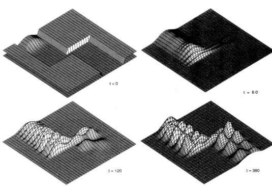
FIG.

4. The development of the wave function in an electron waveguide with akink. Thefigure shows the square magnitude ofthe

wave function on a32x 128 sim-ulation mesh. The boundary re-gion has alength ofn

=

8,and the wavelength ofthe injected wave is approximately 14mesh units. The scaled value oftime isindicated on the figure. The potential profile issuperimposed onthe wave func-tion for t

=

0. The oscillations inthe outgoing channel are due to the interference between the com-ponents ofthe electron wave func-tion in the first and the second subbands.

direction and in the eigenstate

u(l„,

l,

) near the bound-ary. The integers

l,

I,

„,

/ label the position coordinates

on the three-dimensional mesh, and the expansion coeffi-cients

cy(l„,

l,

) may be determined as before for fixed

l„

and I

.

Three applications of the boundary conditions are dis-played in Figs. 1—

4.

(All computations have been carried out using single precision arithmetic. ₎ Figure 1 displays the motion of an initially Gaussian wave packet with a momentum in the

+x

direction, in the presence ofa per-fectly reflecting boundary

at

l

=

1,

and a perfectly ab-sorbing boundary

at

l

=

33.

The accuracy of the wave packet leaving the boundary

at

the scaled time value of 15 has been checked against

a

simulation

of

the same wave packet on a mesh which extends

to

128 points. At this value

of

the scaled time, one expects no errors on this larger mesh due to the boundary condition, as the wave packet is

a

safe distance away from the boundary. The

"error"

in the wave packet on the smaller mesh in comparison

to

that on the larger mesh is displayed in

Fig. 2.

As apparent in this figure, there is a dramatic improvement in the approximation as the size n of the boundary region is increased, in fact at the scale of

Fig. 1,

the wave function generated with n

=

8 and 16 are indis-tinguishable from the one generated on the larger mesh. A boundary size corresponding

to

n

=

8 seems to be op-timal for

a

large class of problems in terms of accuracy-computational resource tradeoff

Figure 3shows the progress

of

awave injected into an initially empty space containing a tunneling barrier. A Gaussian wave front has been imposed onthe wave. The results of the simulation implementing the method de-scribed above have been compared with the results of a simulation carried out on a periodic mesh

of

size

4096.

Again, this large mesh avoids the problems associated with boundary conditions for the values of the time vari-able indicated in the figure. The difference between the

results

of

the two simulations is not visible in the scale

of

the figure, two insets are provided

to

display this dif-ference

at

an expanded scale.

The method has been tested for

a

large class of prob-lems corresponding

to

various potential functions and ini-tial conditions.

It

was found

to

be robust in these appli-cations.

The boundary condition described in this work has also been applied

to

two-dimensional systems in which the wave function is incident (and absorbed) through chan-nel like potentials.

By

carrying out an ensemble ofsingle particle simulations (each corresponding to a different incident wave) in parallel,

it

is possible to study quan-tum transport through two-dimensional structures in the presence of time-dependent boundary conditions. Fig-ure 4 displays the progress of the wave function through

a

kink (or "double-bend") shaped channel at different times. This structure isexpected

to

have interesting non-linear transport properties. The results of this study will be reported elsewhere.

An implementation ofabsorbing and injecting bound-ary conditions for numerical simulations

of

the time-dependent Schrodinger equation has been described. The method is Markovian and isstable under alarge range of conditions. The basic idea is probably applicable

to

other types ofwave equations (such as the Maxwell Equations) although we have not tested this.

An important practical point is the application

of

the fast Fourier transform

to

the solution of the wave equa-tion for systems with open boundaries, which results in improved numerical efficiency. There may bepossibilities for improvement in the method, for example through a difIerent choice ofmomentum components that are spec-ified in the extrapolation procedure, or indeed possibly through the adaptation

of

a totally diferent extrapo-lation procedure. The removal of the sharp cutofFs in space and momentum are areas

of

possible improvement.

The method described above is presently being used in

a

more demanding study

of

atwo-dimensional system in the presence

of

aselfconsistent potential. This work will be reported separately.

The authors would like

to

thank Erkan Tekman for many &uitful discussions and a critical reading of the manuscript.

C. S. Lent and D.

J.

Kirkner,

J.

Appl. Phys. O'_7, 6357

(1990).

R.

Landauer, IBM

J.

Res. Dev.

1,

223

(1957).

B.

Engquist and A. Majda, Math. Comput.

Sl,

629(1977).

R.

K. Mains and G.

I.

Haddad,

J.

Appl. Phys. O4, 3564 (1988).

R. K.

Mains and G.

I.

Haddad,

J.

Appl. Phys. OF, 591

(1990).

T.

Shibata, Phys. Rev.

B

48, 6760

(1991).

J.

-P.Kuska, Phys. Rev.

B

46, 5000

(1992).

L.

F.

Register, U.Ravaioli, and

K.

Hess,

J.

Appl. Phys.

69,

7153

(1991);71,

1555(E)(1992).

See Appendix D of Ref. 10 for a discussion of difBcul-ties involving boundary conditions on the time-dependent Schrodinger equation.

W. R.Frensley, Rev. Mod. Phys. 62, 645

(1990).

J.

R.

Hellums and W. R.Frensley, Phys. Rev.

B 49'

2904

(1994).

K.

Stratfort and

J.

L.Beeby,

J.

Phys. Condens. Matter 5, L289

(1993).

P.Carruthers and

F.

Zachariasen, Rev. Mod. Phys.

55,

245 (1983).

Although the procedure to be described here in relation to the boundary condition is probably applicable to other

widely used updating methods, this point was not verifj.ed. See, for example, G.Dahlquist and A. Bjorck, Numerical Methods (Prentice Hall, Englewood Cliffs, NJ, 1974), p. 284.

G. Dahlquist and A. Bjorck, in Numerical Methods (Ref. 15), p. 102.

"M.

C.Yalabxk, in Negative Differential Resistance and In stabilities in 2-D Semiconductors, N. Balkan,

B.

K.Ridley, and A.

J.

Vickers (Plenum, New York, 1993),pp. 171—178.