Solving a stability problem by Polya's four steps

Volume 1. Number.1 pp.(19-28)

SOLVING A STABILITY PROBLEM BY POLYA’S FOUR

STEPS

Cengiz Alacacı

1

Murat Doğruel

1

1_{Bilkent University, Graduate School of Education, 34722G269, Bilkent, 06800 Ankara,Turkey}

E-mail: alacaci@bilkent.edu.tr

2_{Marmara University, Faculty of Engineering, Goztepe, Istanbul}

Abstract: In this paper, we consider the proof of stability of a nonlinear system. We found it useful to employ

Polya’s general four step problem solving process to organize and present the solution and our thinking. Polya's ideas can help us become aware of how we think when we solve problems. Reflecting on how we solve a problem allows us make conceptual connections between a problem at hand and the problems we may need to solve in the future.

Key Words: Saturation Nonlinearity, Lyapunov stability, Teaching problem solving and heuristic strategies

I. INTRODUCTION

Stability problems are important in engineering, especially in designing control systems. Solving stability problems may require extensive use of mathematical analysis. Methods of solution are sometimes more than straightforward applications of familiar algorithms. The problems and their solutions require intuition, experimentation, trial and error and active monitoring of one’s thinking.

In presenting mathematical solutions of many engineering problems, most scholarly papers and textbooks treat the solution as a finished product, giving little insight into the processes of solution. There is often little exposition of the choices made, why they were made, and little reflection on the solution once it is reached. As George Polya said in his well-known book How to solve it, “Teachers and

authors of textbooks should not forget that the intelligent student and the intelligent reader are not satisfied by verifying that the steps of reasoning are correct but also want to know the motive and the purpose of the various steps.” [7, p. 50]. We believe

that there is value in consideration of these aspects of “thinking about thinking” in solving problems.

Most experienced problem solvers agree that relating the problem at hand to similar problems, understanding it, choosing a method of approach, knowing when to back off and reconsider the method when it seemed unproductive, and looking back and

reflecting on the solution are critical parts of the solution process. Readers of a problem solution would benefit from discussion of these issues as much as the products of the solution, because it helps to give a deeper understanding of the solution. For novices, it makes attainment of these self-regulatory skills less of a solitary experience.

In this article, we present a solution of a stability problem. We found it useful to employ George Polya’s (1887-1985) general four step problem solving process to organize and present the solution and our thinking. The steps of solving a problem are outlined in his well-known book “How

to Solve It” [7]:

1. Understanding the problem, 2. Devising a plan,

3. Carrying out the plan, 4. Looking back.

The first step involves understanding the given conditions and constraints of the problem,

elaborating the goal and the unknown, making the necessary assumptions. The second step requires consideration of similar problems solved before, if the problem can be worded differently to make it more familiar, and eventually developing a plan of attack. The third step involves applying the procedures of the chosen method and making sure that it is used correctly. In the last step, findings are tested against the conditions of the problem, and connections with similar problems of more general type are made based on the findings.

The steps may not be used in a fixed order. .For example, if problems are encountered while carrying out the plan, individual may need to go back and revise the plan, or even return to the first step to make additional assumptions in order to use a particular method [9]. It is important to note that we use Polya’s steps of problem solving as a tool of illustrating, organizing, and presenting our thinking, rather than a specific method of solution by itself.

II. THE PROBLEM

“Solving problems is a fundamental human activity. In fact, the greater part of our conscious thinking is concerned with problems.” [7, p. 221]

As an example, consider the following specific system provided in [3]:







+

−

−

=

+

+

=

,

,

2 1 2 2 1 1

u

x

x

x

u

x

x

x

&

&

(1) with a saturated linear control function

)

475

.

0

625

.

0

(

x

₁

x

₂

sat

u

=

−

−

, where

.

1

,

1

,

1

|

|

,

1

,

1

,

)

(

−

<

>

≤











−

=

α

α

α

α

α

sat

The problem is to find out if the above system is globally asymptotically stable.

III. UNDERSTANDING THE

PROBLEM

“The intelligent problem-solver tries first of all to understand the problem as fully and as clearly as he can. … The open secret of real success is to throw your whole personality into your problem.” [7, p.

173]

Our first duty is to understand the problem [7, p173]. If there was no saturation, the system would be completely linear, and we could have checked the global asymptotic stability by just seeing if the eigenvalues of the feedback system have negative real parts. Anyhow, let us check them and have an idea about the system. When there is no feedback (u=0), the open loop system eigenvalues are both located at 0, and they are coupled. This is a little bit alarming because this kind of system is potentially unstable. Assuming there is no saturation, with the linear feedback, the system eigenvalues are moved to -0.5 and -0.6 which would produce a stable system. This linear feedback is only valid in the unsaturated region where

1

475

.

0

625

.

0

1

≤

−

1

−

2

≤

−

x

x

.

This region, on the other hand, includes the origin, where the state variable will eventually reach. This suggests that the system (1) with the feedback is asymptotically stable. To show that it is globally asymptotically stable, we further need to show that all trajectories starting at any initial position in the state space will actually reach the origin.

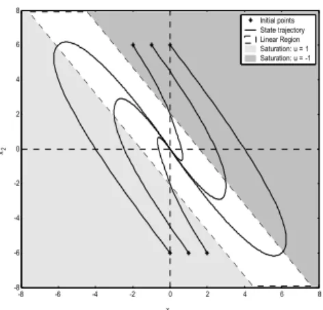
Let us elaborate on the problem further. We should simulate the system to understand its behavior. Figure 1 shows trajectories for various initial conditions. As expected, the system shows a stable behavior at least locally. To see the behavior in the large, we simulate the system for an initial value of (25, 25) as shown in Figure 2. The corresponding saturated control is depicted in Figure 3.

-8 -6 -4 -2 0 2 4 6 8 -8 -6 -4 -2 0 2 4 6 8 x 1 x2 Initial points State trajectory Linear Region Saturation: u = 1 Saturation: u = -1

Fig. 1.

State trajectories of the nonlinear system for various initial values.

-400 -300 -200 -100 0 100 200 300 400 500 600 700 -700 -600 -500 -400 -300 -200 -100 0 100 200 300 400 x1 x2 Initial point State trajectory

Fig. 2.

The state trajectory for an initial value of (25, 25). 0 20 40 60 80 100 120 140 -1 -0.5 0 0.5 1 t (sec.) u

Fig. 3.

The control input versus time (in seconds) for an initial value of (25, 25).

As seen in Figure 2, although the trajectory starts at (25, 25), it first moves to around (600, -600) then to (-300, 300) and eventually stabilized at the origin. Of course, one example would not be sufficient, but our intuition says that although the trajectory moves and oscillates too much, the system could be globally stable.

In order to obtain a simpler system representation, a linear transformation can be applied. From (1), it is easily seen that

x

&

1

+ &

x

2

=

2

u

. Hence, if one of the

state variables is chosen as

(

x +

₁

x

₂

)

/

2

, its

derivative will be simply

u

. Also

)

(

2

_{1 2} 2 1

x

x

x

x

&

− &

=

+

or

4

/

)

(

2

/

)

(

x

₁

+

x

₂

=

x

&

₁

−

x

&

₂ .

Therefore if the second state variable is chosen as

4

/

)

(

x −

₁

x

₂ , its derivative will be simply the first state variable. Using this idea, let us try the following transformation:







+

=

−

=

.

2

/

)

(

,

4

/

)

(

2 1 2 2 1 1

x

x

y

x

x

y

(2) Now, the following equivalent system is obtained,







−

−

=

=

).

1

.

1

3

.

0

(

,

2 1 2 2 1

y

y

sat

y

y

y

&

&

(3) Since the transformation (2) is invertible, the systems (1) and (3) are equivalent in the global asymptotic stability. The system (3) on the other hand looks a little simpler. We know that the system (3) must also be asymptotically stable locally, but is it globally stable? We simulate the system (3) for an initial value of (0, 75) as shown in Figure 4. -3000 -2000 -1000 0 1000 2000 3000 -80 -60 -40 -20 0 20 40 60 80 y₁ y2 Initial point State trajectory Switching Line

Fig. 4.

The state trajectory for the system (3) for an initial value of (0, 75).

The trajectory path now appears easier to follow. The linear region where

1

1

.

1

3

.

0

1

≤

−

₁

−

₂

≤

−

y

y

,

looks so thin for large y values that it is shown as a dotted line in Figure 4. Outside this linear region, saturation occurs. When the trajectory hits the linear region, it quickly changes its

direction and follows the other saturated dynamics as seen in Figure 4.

IV. DEVISING A PLAN

“To devise a plan, to conceive the idea of the solution is not easy. It takes so much to succeed; formerly

acquired knowledge, good mental habits,

concentration upon the purpose, and one more thing: good luck.” [7, p. 12]

How can then we show that the system is actually globally stable? There are some methods to try in our toolbox. The famous circle or Popov criteria (for example see [10] or [4]) would be a suitable method for this problem; however the open loop system has coupled eigenvalues on the jw axis. Loop transformation (see [4]) will not work either because the saturation nonlinearity belongs to the sector [0 1]. In fact, for this kind of systems there are some nonlinearities in sector [0 1] that makes the system globally unstable (see Example 7.1 in [6]); therefore the system is actually not absolutely globally stable, therefore these methods are not applicable. There is, actually, a result to show the global stability of this specific system in the literature (for example see [2],[1],[8]), however, let us continue on our path since our main goal is to show a solution strategy of the problem.

A very well-known method to show global stability is Lyapunov’s direct method ([10], [4]). Let us try to use this classical and powerful method. The level surfaces of the Lyapunov function (for a fixed function value) must be in such a way that when the trajectory enters in the surface, it must never leave that surface. To be able to guess a proper Lyapunov function for this example, we need to understand how exactly the trajectory moves when it is in the saturated regions.

On the right side of the linear region (for

−

0

.

3

y

1

−

1

.

1

y

2

<

−

1

),the corresponding system dynamics is







−

=

=

.

1

,

2 2 1

y

y

y

&

&

(4) And, on the left side

(for

−

0

.

3

y

₁

−

1

.

1

y

₂

>

1

), we have







=

=

.

1

,

2 2 1

y

y

y

&

&

(5) The solutions of these systems can be easily found as follows.

For the system (4):







+

−

=

+

+

−

=

).

0

(

)

(

),

0

(

)

0

(

)

(

2 2 1 2 2 2 1 1

y

t

t

y

y

t

y

t

t

y

(6) For the system

(5):







+

=

+

+

=

).

0

(

)

(

),

0

(

)

0

(

)

(

2 2 1 2 2 2 1 1

y

t

t

y

y

t

y

t

t

y

(7)

Therefore we conclude that outside the linear region the trajectories follow a parabolic path. Another observation, from Figure 4, is that although the intersections of the trajectory with the y2 axis grow

linearly as y2 is increased, the intersections grow

approximately in square fashion for the y1 axis.

Through these observations we can conclude that

V(x) = x’Px type quadratic Lyapunov function

candidates are not suitable for this nonlinear system. The reason is that a quadratic function produces elliptic level surfaces which have a fixed width/height ratio. In this case however, the level surfaces should be in such a way that the width/height ratio should grow for a higher Lyapunov function value.

“Devising the plan of the solution, we should not be too afraid of merely plausible, heuristic reasoning. Anything is right that leads to the right idea.” [7, p.

68]

Then, how can we find a proper Lyapunov function for this example? From the simulations, and from (6) and (7), we observe that in either one of the saturation regions and for a certain portion of the trajectory, the quantity

y +

₂2

2 y

₁ remains constant. This may be a good start for a Lyapunov function candidate. Let 1 2 2

2

)

(

y

y

y

V

=

+

, (8) and check how it behaves for the system (3). Using the same initial value as in Figure 4, the function (8) is shown in Figure 5. It almost works; there is no increase in the function, and it stays constant on the parabolic paths as expected. However, the function must be strictly decreasing to show the global stability.

0 100 200 300 400 500 600 700 800 900 1000 0 1000 2000 3000 4000 5000 6000 t (sec.) V

Fig. 5.

The Lyapunov function candidate (8) for an initial state value of (0, 75).

How can we make the function decrease when the trajectory moves on the parabolic path? We observe that y2 increases for the left region, and decreases for

the right region when the time moves forward. Using this hint, we suggest this new Lyapunov function candidate 2 1 2 2

2

)

(

y

y

y

ky

V

=

+

+

. (9) After some simulations, we see that this candidate seems to work for positive k values less than 6.4. For

k=1, the resulting function is shown in Figure 6. Now

we have a strictly decreasing Lyapunov function candidate for the system (3).

0 100 200 300 400 500 600 700 800 900 1000 0 1000 2000 3000 4000 5000 6000 t (sec.) V

Fig. 6.

The Lyapunov function candidate (9) for an initial state value of (0, 75).

One problem with (9) is that it does not have continuous first order derivatives due to the absolute value operator. To fix this problem, we may substitute the following smoother function in place of

the absolute value function

,

1

|

|

,

1

|

|

,

|

|

,

)

(

|

|

2 1 2 2 1 0

>

≤







−

=

∫

≅

z

z

z

z

d

sat

z

z

α

α

which has continuous first order derivatives, and for larger values (

z

>

1

), approximately does the same job as an absolute value function. Therefore, choosing k=1, we suggest a Lure-type Lyapunov

∫

+

=

2 1+ 2 0 2 2

(

)

)

(

y y

d

sat

y

y

V

α

α

, (10)

which behaves approximately the same as shown in Figure 6. Simulations fortunately shows that, for small y values around the origin, in the linear region, (10) still works as a proper Lyapunov function. Finally, using the transformation (2) and the candidate (10), the corresponding Lyapunov function candidate for the system (1) can be found as

∫

+

+

=

1 0 2 2 1 4 1

₍

₎

₍

₎

)

(

x

d

sat

x

x

x

V

α

α

. (11)

We expect that the global asymptotical stability of the system (1) should be shown using this function.

IV. CARRYING OUT THE PLAN

“To carry out the plan is much easier; what we need is mainly patience. The plan gives a general outline; we have to convince ourselves that the details fit into

the outline, and so we have to examine the details one after the other, patiently, till everything is perfectly clear, and no obscure corner remains in which an error could be hidden.”

[7, p. 12-13]

Now, we need to prove that the candidate (11) is really a proper Lyapunov function for global asymptotic stability (for example see Theorem 3.3 in [4]). It is easy to see that

V

( x

)

is positive definite and radially unbounded, and has continuous first order derivatives. Using the system equations, we have

(

)

(

)

).

475

.

0

625

.

0

(

)

(

)

475

.

0

625

.

0

(

)

(

*

*

)

(

,

)

475

.

0

625

.

0

(

*

*

)

(

)

475

.

0

625

.

0

(

*

*

)

(

,

)

(

)

)(

(

)

(

2 1 1 2 1 1 2 1 2 1 2 1 1 2 1 2 1 1 1 2 1 2 1 2 1

x

x

sat

x

sat

x

x

sat

x

sat

x

x

x

x

sat

x

x

x

sat

x

x

sat

x

x

x

x

sat

x

x

x

x

x

V

−

−

+

−

−

+

+

=

−

−

+

+

+

−

−

+

=

+

+

+

=

&

&

&

&

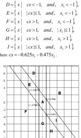
Let us first formally define the regions shown in Figure 7,

{

}

{

}

{

}

{

}

{

}

{

}

{

}

{

}

{

|

|

1

,

,

1

}

.

,

1

,

,

1

,

1

|

|

,

,

1

,

1

,

,

1

,

1

,

,

1

|

|

,

1

,

,

1

,

1

|

|

,

,

1

,

1

,

,

1

,

1

|

|

,

,

1

|

|

1 1 1 1 1 1 1 1 1

>

≤

=

>

>

=

≤

>

=

−

<

>

=

−

<

≤

=

−

<

−

<

=

≤

−

<

=

>

−

<

=

≤

≤

=

x

and

cx

x

I

x

and

cx

x

H

x

and

cx

x

G

x

and

cx

x

F

x

and

cx

x

E

x

and

cx

x

D

x

and

cx

x

C

x

and

cx

x

B

x

and

cx

x

A

where

cx

=

−

0

.

625

x

₁

−

0

.

475

x

₂.

Fig. 7.

The regions for the Lyapunov function (11). In region A:

(

)

. 0 || || for 0 1444 . 0 ) 575 . 0 5 . 0 ( , 475 . 0 575 . 0 25 . 0 ), 475 . 0 625 . 0 ( 475 . 0 625 . 0 ) ( ) ( 2 2 2 2 1 2 2 2 1 2 1 2 1 1 2 1 1 2 1 ≠ < − + − = − − − = − − + − − + = x x x x x x x x x x x x x x x x x V& And

V&

(

0

)

=

0

.

In region B:

(

1

1

)

1

(

1

)

1

0

.

)

(

)

(

x

=

x

₁

+

x

₂

−

+

−

=

−

<

V&

In region C:

(

)

(

1

)

1

0

)

1

(

)

1

(

1

)

(

)

(

0 1 0 2 1 1 1 2 1

<

−

−

−

+

=

−

+

−

+

=

≤ >

43

1

2

3

42

1

&

x

x

x

x

x

x

x

x

V

. In region D:

(

)

0

)

(

2

1

)

(

2

)

1

(

1

1

1

)

(

)

(

0 2 1 2 1 2 1 2 1

<

−

+

−

=

+

+

−

=

−

−

−

−

+

=

>

43

42

1

&

x

x

x

x

x

x

x

V

. In region E:

(

)

2 1 2 2 2 1 2 1 2 1 2 1 2 1 525 . 0 375 . 0 475 . 0 1 . 1 625 . 0 ), 475 . 0 625 . 0 ( 1 475 . 0 625 . 0 1 ) ( ) ( x x x x x x x x x x x x x V − − − − − = − − − − − − + = &

In regions F to I: Since

V

&

(

x

)

= &

V

(

−

x

)

, and

0

)

(

x

<

V&

in the opposite regions,

V&

(x

)

must also be negative in these regions.

Hence,

V&

(x

)

is a negative definite function. Therefore we conclude that the system (1) with the saturated linear feedback is actually globally asymptotically stable.

VI. LOOKING BACK

“Looking back at the completed solution is an important and instructive phase of the work. ‘He thinks not well that thinks not again.’ ‘Second thoughts are best.’ ” [7, p.224]

Looking back the problem, according to Polya, we need to ask these questions [7]:

• Can you derive the solution differently?

• Can you use the result, or the method, for

some other problem?

Here, we have considered a specific problem, however we may use the solution strategy and the insights we gained from it in a general statement of the problem. Let us reconsider (3) with general parameters,







+

−

=

=

).

(

,

2 2 1 1 2 2 1

y

k

y

k

sat

y

y

y

&

&

(12) Here

k

₁ and

k

₂ are assumed to be positive constants, otherwise the system will not be asymptotically stable, because locally the corresponding linear system will not have both eigenvalues in the left half plane. For any positive

1

k

and

k

₂, on the other hand, the system will be guaranteed to be asymptotically stable locally. To understand the global behavior in general, let us consider Figure 8, as done for the specific case in Figure 4. y₁ y2 (1 ) (1 ) (1 ) (1 ) (2) (2) (2) (2) (3) (3) (3) (3) y₂= -(k₁/k₂)y₁ p_r -p l

Fig.8.

The general state trajectory in the large. As before, the linear region looks so thin in the large view that it is shown as a dotted line in Figure 8. Assuming the initial state is sufficiently large, we see that trajectory starting at point (1) follows a parabolic path, and reaches point (2). Then it follows another parabolic path and reaches point (3). The formulas (6) and (7) will also apply here for the general case. Then, the trajectory continues in a similar way until it reaches the origin. This suggests that for any positive

1

k

and

k

₂, the system (12) should be globally asymptotically stable. However, how can we prove this result? In the earlier specific problem, we spent too much effort to find and prove a proper Lyapunov function.

Using (6) and (7), the parabolic trajectory paths can be obtained as,

For the system (4) (the right side):

y

=

−

y

2

+

p

_r

2 2 1

1 ,

(13)

For the system (5) (the left side):

y

=

2

y

22

−

p

_l

1

1 ,

(14)

where pr and -pl are the points that the trajectory

crosses y1 axis on the right and left sides. Actually the

values pr and pl can be good measures for the

“energy” or “size” of the parabolic trajectory. Perhaps we can use these values to construct the Lyapunov function. Therefore, using (13) and (14), let us suggest a Lyapunov function candidate as

. 1 , 1 , , ) ( 2 2 1 1 2 2 1 1 2 2 2 1 1 2 2 2 1 1 − < + > +    + − + ≅ y k y k y k y k y y y y y V (15)

Actually this function may not even be positive definite (especially when k1/k2 is small), however, let

us not stop and get discouraged, but go on and try to improve the function step by step if possible. The two cases in the above formula can be combined as shown below,

),

(

)

(

2 _{1 1 1 2 2} 2 2 1

_y

_y

_sat

_k

_y

_k

_y

y

V

=

+

+

(16) where the sat() function automatically handles the sign of y1 in (15). Therefore when the trajectory is on

the parabolic path, V(y) will be constant; and when the trajectory reaches the other side, it will be reduced almost instantly as observed in Figure 5. Again, y2 can be used to obtain a decreasing V(y) as,

), ( ) ( ) ( 1 2 1 1 2 2 2 2 2 1_{y y y sat k y k y} y V = + +

σ

+ (17)

where

σ

is a positive constant so that, on the right side, V should decrease since y2 decreases. On the left

side, y2 increases, but because of the negative sign of

the sat() function, V should again decrease. To ensure that the function in (17) is a positive definite function for any (positive)

k

₁ and

k

₂, the parameter

σ

can be chosen as k2/k1, therefore one obtains

).

(

)

(

1

)

(

_{1 1 2 2 1 1 2 2} 1 2 2 2 1

_k

_y

_k

_y

_sat

_k

_y

_k

_y

k

y

y

V

=

+

+

+

(18)

Note that

z ⋅

sat

( z

)

is always positive for

z

≠

0

. Now the problem, as before, is that V must have continuous first order derivatives.

To overcome this problem, the following approximation can be used,

∫

≅

⋅

sat

z

z

sat

d

z

0

)

(

)

(

α

α

and finally the following Lyapunov function candidate can be suggested,

.

)

(

1

)

(

11 2 2 0 1 2 2 2 1

+

_∫

=

ky+ yk

sat

d

k

y

y

V

α

α

(19)

“Examining the various parts, one after the other, and trying various ways of considering them, we may be led finally to see the whole result in a different light, and our new conception of the result may suggest a new proof.” [7, p. 64]

It is clear that V(y) is positive definite and radially unbounded, also it has continuous first order derivatives. Let us check its derivative,

.

0

)

(

)

(

)

(

)

(

)

(

2 2 1 1 2 1 2 2 2 1 1 2 1 2 2 2 1 1 2 2 2 1 1 2

≤

+

−

=

+

−

+

+

+

−

=

y

k

y

k

sat

k

k

y

k

y

k

sat

k

k

y

k

y

k

sat

y

y

k

y

k

sat

y

y

V&

(20)

It is easily seen that

V&

( y

)

is negative semidefinite; and for the points satisfying

k

₁

y

₁

+ y

k

_{2 2}

=

0

(the linear line in Figure 8),

V&

( y

)

is zero. Since

V&

( y

)

is only negative semidefinite, the invariant set theorem can be applied (see Theorem 3.5 in [10]). In fact, according to (12), for any initial state starting on the invariant set (the points on the linear line), the corresponding trajectory immediately leaves the invariant set, except for the origin. Hence, we conclude that the origin of the system (12) is globally asymptotically stable for any positive

k

₁ and

k

₂. Therefore using the Lyapunov function (19) instead of (11), the stability is proven in a much easier way, and for a general system.

Let us generalize the system representation even further, as







+

−

=

=

).

(

,

2 2 1 1 2 2 1

y

k

y

k

f

y

y

y

&

&

(21) Here a general nonlinear function is used instead of the saturation. Adapting (19) for this case, we can suggest

∫

+

=

11+2 2 0 1 2 2 2 1

1

₍

₎

)

(

y k y k

d

f

k

y

y

V

α

α

, (22) and therefore,

)

(

)

(

1 1 2 2 2 1 2

y

k

y

k

f

k

k

y

V

&

=

−

+

. (23)

If the following conditions are satisfied,

then the Lyapunov function (22) will be positive definite (conditions 2 and 4), radially unbounded (condition 3), having continuous first order derivatives (condition 1); and, the derivative (23) will be negative semidefinite (condition 4), and zero only on the line

k

₁

y

₁

+ y

k

_{2 2}

=

0

(condition 2). Again, according invariant set theorem, we can conclude the following result:

The system (21) satisfying the conditions (24), is globally asymptotically stable.

Actually many systems in practice can be reduced to

the system description in (21). Many

electromechanical systems can be described as a double integrator type dynamics with linear negative feedback through a nonlinear and/or saturating actuator. One example for such f(x) is shown in Figure 9. It should be noted that, although this kind of systems are globally asymptotically stable, the trajectories may easily pass over the practical limits in the state space as observed in Figure 2.

1)

f

( x

)

is continuous, 2)

xf

(

x

)

>

0

for

x

≠

0

(and

f

(

0

)

=

0

), 3)

∫

f

α

d

α

→

∞

x 0

)

(

as

x

→

∞

, 4)

k

₁

>

0

, and

k

₂

>

0

.

Fig.9.

An example of a nonlinear function satisfying the conditions 1-3 in (24).

It is also interesting to note that when there are three or more cascaded integrators, no linear saturated

feedback will produce a globally asymptotically

stable system [11]. According to the result found, when there are two cascaded integrators (double integrators), all the stabilizing linear feedbacks will work for the saturated case.

The result presented here could not be found on many books or papers on nonlinear systems. For example, [10] (Example 3.14), [4] (Example 4.9), and [6] (Example 6.5) only mentions that the systems in the following form are globally asymptotically stable:







−

−

=

=

),

(

)

(

,

2 1 2 2 1

y

g

y

f

y

y

y

&

&

where f satisfies the conditions 1-3, and g satisfies the conditions 1-2 in (24). As indicated in [8], Meyer studied the linear systems with two zero eigenvalues and saturated linear control, and gave conditions on the global asymptotic stability (see pp.53-54 in [5]). Although it is not shown explicitly, when (21) is considered as a special case, Meyer’s conditions reduce to (24). Also in an exercise (p.65 in [1]), Aggarwal suggests a similar Lyapunov function as in (22) for the system (21). Many different control methods and stability results for double integrators are presented in [8].

VII. CONCLUDING COMMENTS

“The author remembers the time when he was a student himself, a somewhat ambitious student, eager to understand a little mathematics and physics. He listened to lectures, read books, tried to take in the solutions and facts presented, but there was a question that disturbed him again and again: “Yes, the solution seems to work, it appears to be correct;

but how is it possible to invent such a solution? Yes, this experiment seems to work, this appears to be a fact; but how can people discover such facts? And how could I invent or discover such things by myself?” … Trying to understand not only the solution of this or that problem but also the motives and procedures of the solution, and trying to explain these motives and procedures to others, he was finally led to write the present book.” [7, from introduction]

In this article, we attempted to present the plausible reasoning that Polya described. We tried to expose the thinking that went into solving a saturation nonlinearity type stability problem with specified parameters. In order to solve it, we needed to understand the effect of the nonlinearity on the linear system, and explore its behavior. For example, to understand the problem, we simulated the system in various initial conditions. Then we looked into plausible methods and chose the one that seemed to satisfy the constraints of the problem. Popov criterion could not be applied even with a loop transformation, but Lyapunov method seemed promising. After considerable experimentation, we were able to find a function that helped demonstrate the global stability of the problem and we verified the findings. Looking back, based on the insights gained from solving the specific version of the problem, we posed a new question: What if the parameters are considered in general as k1 and k2? Using a similar solution

strategy, but finding a more convenient Lyapunov function this time, we could prove the global stability for the general case. By simply adapting the Lyapunov function, we were able to demonstrate the global stability of the more general case when the saturation is replaced by a special nonlinear function. We moved from specific to a general case in this problem. Technically, the more general solution subsumes the specific solution, but this should not take away from the value of the findings to the specific case. Because reaching the general solution was based on the findings of the specific case. We are hoping that the inductive solution we present here can provide a glimpse of the thinking that produced the results which are often given deductively as a finished product in most scholarly writings.

By its nature, Polya's ideas can help us become aware of how we think when we solve problems. By reflecting on how we solve a problem, we are more likely to make connections with the problem at hand and the problems we may need to solve in the future. Being well-versed in Polya's ideas and steps may not by itself guarantee success in understanding or solving a new problem, because such success is a product of both knowledge of similar problems and how we regulate that knowledge and our mental resources. However, Polya’s ideas can help unpack the complex thinking processes that go into the solution of a problem, and hence can help the novices develop effective self-regulating skills in thinking to re-produce the solution and produce new solutions to other problems.

VIII.REFERENCES

[1] J.K. Aggarwal: Notes on Nonlinear Systems, New York, Van Nostrand Reinhold, 1972.

[2] J. Alvarez, R. Suárez and J. Alvarez: “Planar linear systems with single saturated feedback,” Systems & Control Letters, 20, 319-326, (1993). [3] M. Doğruel: “Input linearization of nonlinear systems via pulse width control,” IEEE Transactions on Automatic Control, 48(4), 635-638, (2003). [4] H.K. Khalil: Nonlinear Control Systems, Third Ed., Englewood Cliffs, Prentice Hall, 2002.

[5] S. Lefschetz: Stability of Nonlinear Control Systems, New York, Academic Press, 1965.

[6] R.R. Moher: Nonlinear Systems, Volume I, Dynamics and Control, Englewood Cliffs, Prentice Hall 1991.

[7] G. Polya: How to Solve It, A New Aspect of

Mathematical Method, Second Ed., Princeton,

Princeton University Press 1985.

[8] V. Rao and D. S. Bernstein: Naive Control of the Double Integrator, IEEE Control Systems Magazine, 21, 86-97, (2001).

[9] A.H. Schoenfeld: Cognitive Science and Mathematics Education, Hillsdale, Lawrence Erlbaum 1987.

[10] J.E. Slotine and W. Li: Applied Nonlinear Control, Englewood Cliffs, Prentice Hall 1991. [11] H.J. Sussmann and Y. Yang: On the stabilizability of multiple integrators by means of bounded feedback controls, Proc. 30th CDC, pp. 70-72, Brighton, U.K. (1991).