SHIPMENT CONSOLIDATION UNDER
DIFFERENT DELIVERY DATE OPTIONS FOR
E-TAILING
a thesis submitted to
the graduate school of engineering and science
of bilkent university
in partial fulfillment of the requirements for
the degree of
master of science
in
industrial engineering
By
Tu˘
g¸ce Vural
SHIPMENT CONSOLIDATION UNDER DIFFERENT DELIVERY DATE OPTIONS FOR E-TAILING
By Tu˘g¸ce Vural June, 2015
We certify that we have read this thesis and that in our opinion it is fully adequate, in scope and in quality, as a thesis for the degree of Master of Science.
Prof. Dr. Nesim K. Erkip(Advisor)
Prof. Dr. ¨Ulk¨u G¨urler
Assoc. Prof. Osman Alp
Approved for the Graduate School of Engineering and Science:
Prof. Dr. Levent Onural Director of the Graduate School
ABSTRACT
SHIPMENT CONSOLIDATION UNDER DIFFERENT
DELIVERY DATE OPTIONS FOR E-TAILING
Tu˘g¸ce Vural
M.S. in Industrial Engineering Advisor: Prof. Dr. Nesim K. Erkip
June, 2015
In this thesis, we consider a shipment consolidation problem for an e-retailer company which has two type of services for its customers: “regular” and “premium”. In the regular service, the e-retailer guarantees a delivery time to its customers. However, in the premium service, customers get their items in negligible or zero amount of time, such as same-day delivery, supplied physical inventories located sufficiently close. When a shipment decision is made, it serves both customers of the regular service and small inventories for the premium service. In our study, we analyze shipment consolidation operation given these two services for both deterministic and stochastic demand structure. In the deterministic demand problem, our average profit maximizing model decides the optimal service choice; we provide optimality conditions, an algorithm to find optimal solution, structural analyses and numerical results. In the stochastic demand setting, we evaluate the problem for the regular service which has Poisson demand. Then, we expand the problem by including the premium service which has deterministic demand. For this problem, we present an approximate model for a modified version of the policy used for regular-service-only problem and compare the performance of the approximation with a simulation.
¨
OZET
FARKLI SERV˙IS S ¨
URELER˙I ALTINDA E-T˙ICARET
S
¸ ˙IRKETLER˙I ˙IC
¸ ˙IN SEVK˙IYAT OPERASYONU
Tu˘g¸ce Vural
End¨ustri M¨uhendisli˘gi, Y¨uksek Lisans Tez Danı¸smanı: Prof. Dr. Nesim K. Erkip
Haziran, 2015
Bu tezde, m¨u¸steriye malı g¨onderme ¨ozelliklerinin “normal” ve “¨ozel” servis adı altında farklıla¸stıran bir e-ticaret sirketi i¸cin sevkiyat konsolidasyonu problemi ele alınmı¸stır. Nor-mal serviste e-ticaret ¸sirketi m¨u¸sterilerine belli bir teslimat s¨uresini garantilemektedir. ¨Ozel serviste ise ¸sirket satın alınan ¨ur¨unleri anında sayılabilecek bir hızla m¨u¸sterilerine yeter-ince yakın olan bir envanterden tedarik edip teslimat ger¸cekle¸stirilmektedir. Herhangi bir sevkiyat kararı verildi˘ginde, sevkiyat aracı hem normal servisi kullanan m¨u¸sterilere satın aldıkları ¨ur¨unleri ta¸sımakta, hem de anlık tedari˘gi m¨umk¨un kılacak m¨u¸sterilere yakın envan-tere ¨ur¨un ta¸sıyabilmektedir. C¸ alı¸smamızda hem bilinen, hem de rassal talep i¸cin sevkiyat konsolidasyonu operasyonu iki servis ¸ce¸sidi de g¨oz ¨on¨unde bulundurularak analiz edilmi¸stir. Bilinen talep probleminde, modelimiz en iyi servis ¸ce¸sidine karar vererek ortalama karın maksimumunu bulmaktadır. Bu problem i¸cin, eniyilik ¸sartları, en iyi ¸c¨oz¨um¨u bulan algo-ritma, yapısal analizler ve numerik sonu¸clar sunulmu¸stur. Rassal talep modelinde ise, normal servisin m¨u¸sterilerinin Poisson da˘gılımından geldi˘gi varsayılmı¸s ve problem bu varsayımın ¨
uzerinden sadece normal servis i¸cin de˘gerlendirilmi¸stir. Sonrasında, probleme ¨ozel servis, bi-linen bir talep yarattı˘gı varsayılarak dahil edilmi¸stir. Geni¸sletilmi¸s problem i¸cin ise, normal servis i¸cin kullanılan politikanın bu duruma uyarlanmı¸s bir bi¸cimi altında ¸calı¸sacak yakla¸sık bir analitik model ¨onerilmi¸stir. Yakla¸sık modelin performansını g¨ozlemlemek i¸cin bir benze-tim modeliyle kar¸sıla¸stırılmı¸stır.
Acknowledgement
First and foremost, I would like to express my sincere gratitude to my advisor Prof. Nesim K. Erkip for the continuous support of my study and research, for his patience, motivation, enthusiasm, and immense knowledge. I have been amazingly fortunate to have an advisor who gave me the freedom to explore on my own, and at the same time the guidance to recover when my steps faltered.
I am also grateful to Prof. ¨Ulk¨u G¨urler and Assoc. Prof. Osman Alp for their valuable time to read and review this thesis.
I would like to thank Ya˘gız Efe Bayiz for his unique motivation and encouragements.
I am deeply grateful to my mother, Zeliha Vural and my brother, Umurcan Vural for their endless love, everlasting belief and trust in me. Words alone cannot express what I owe them for all their efforts and patience.
Lastly, I would like to dedicate this thesis to memory of my father, Mustafa Vural. His words have been a source of strength, and guidance in my life.
Contents
1 Introduction 1
1.1 Literature Review . . . 3
1.1.1 Background in E-tailing . . . 3
1.1.2 Idea of Shipment Consolidation . . . 5
1.2 Problem Definition . . . 12
2 Shipment Consolidation Problem of E-tailing with Deterministic Demand 16 2.1 Model Description . . . 16
2.2 The Model . . . 24
2.3 Analysis of the Model and the Optimality Conditions . . . 26
2.4 Analysis of KKT Conditions . . . 28
2.5 Solution . . . 30
2.5.1 The Solution Framework . . . 31
2.5.2 The Analysis of Model Subsets . . . 32
2.5.3 Solution Algorithm . . . 33
2.5.4 Verification of the Solution Algorithm . . . 35
3 Analysis of the Shipment Consolidation Problem of E-tailing with Deter-ministic Demand 36 3.1 Numerical Results . . . 36
3.2 Special Cases . . . 41
3.2.1 Ranking Method Proposed For Multi-Item Systems . . . 41
3.2.2 Performance Comparison Method For Different Cases . . . 42
4.1 Shipment Consolidation Problem for Regular Service . . . 49
4.2 Shipment Consolidation Problem Including Premium Service . . . 54
4.2.1 Approximate Model of The Problem with Premium Service . . . 55
4.2.2 Analysis of The Approximate Model . . . 57
4.3 Simulation for The Approximate Model . . . 61
5 Conclusion 64 A An Example For The Objective Function 73 B 32 KKT Cases 75 B.1 Case 1 . . . 76 B.1.1 Case 1.1 . . . 76 B.1.2 Case 1.2 . . . 76 B.1.3 Case 1.3 . . . 77 B.1.4 Case 1.4 . . . 78 B.1.5 Case 1.5 . . . 79 B.1.6 Case 1.6 . . . 80 B.1.7 Case 1.7 . . . 81 B.2 Case 2 . . . 83 B.2.1 Case 2.1 . . . 83 B.2.2 Case 2.2 . . . 83 B.2.3 Case 2.3 . . . 84 B.2.4 Case 2.4 . . . 85 B.2.5 Case 2.5 . . . 86 B.2.6 Case 2.6 . . . 86 B.2.7 Case 2.7 . . . 87 B.3 Case 3 . . . 88 B.3.1 Case 3.1 . . . 88 B.3.2 Case 3.2 . . . 89 B.3.3 Case 3.3 . . . 90 B.3.4 Case 3.4 . . . 90 B.3.5 Case 3.5 . . . 91 B.3.6 Case 3.6 . . . 92
B.3.7 Case 3.7 . . . 93 B.4 Case 4 . . . 94 B.4.1 Case 4.1 . . . 94 B.4.2 Case 4.2 . . . 95 B.4.3 Case 4.3 . . . 95 B.4.4 Case 4.4 . . . 96 B.4.5 Case 4.5 . . . 97 B.4.6 Case 4.6 . . . 97 B.4.7 Case 4.7 . . . 98 C Proof of Proposition 1 100 D K and h Bounds of Some Cases 102 D.1 Case 1.4 . . . 102 D.2 Case 1.5 . . . 103 D.3 Case 1.6 . . . 103 D.4 Case 1.7 . . . 104 D.5 Case 2.1 . . . 105 D.6 Case 2.2 . . . 105 D.7 Case 2.4 . . . 106 D.8 Case 2.5 . . . 106 D.9 Case 2.6 . . . 107 D.10 Case 2.7 . . . 107 D.11 Case 3.1 . . . 108 D.12 Case 3.2 . . . 108 D.13 Case 3.3 . . . 109 D.14 Case 3.4 . . . 109 D.15 Case 3.5 . . . 110 D.16 Case 3.6 . . . 111 D.17 Case 4.2 . . . 111 E Solution 113 E.1 Division of 9 Subsets . . . 113
E.2.1 AX . . . 115 E.2.2 AY . . . 116 E.2.3 AZ . . . 116 E.2.4 BX . . . 117 E.2.5 BY . . . 117 E.2.6 BZ . . . 118 E.2.7 CX . . . 118 E.2.8 CY . . . 118 E.2.9 CZ . . . 119
F MATLAB Code for The Algorithm 120
G Verification of Little’s Law for the Stochastic Demand Problem - Regular
Service Only 136
List of Figures
1.1 Shipment Consolidation . . . 13
2.1 The Regular Policy . . . 17
2.2 The Premium Policy . . . 18
2.3 The Joint Policy . . . 20
2.4 The Regular, The Premium and The Joint Policies . . . 21
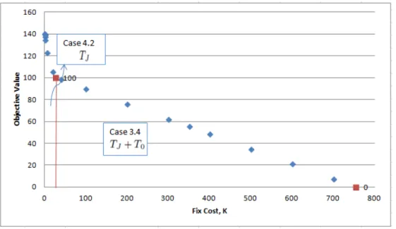
3.1 Fixed Cost vs Optimal Profit . . . 37
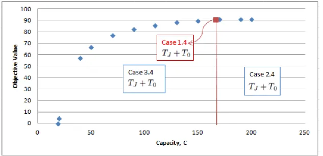
3.2 Capacity vs Optimal Profit . . . 38
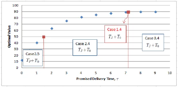
3.3 Promised Delivery Time vs Optimal Profit . . . 39
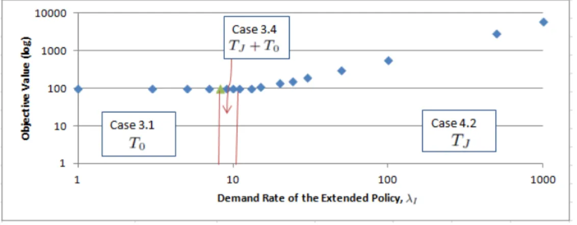
3.4 λP vs Objective Profit when K=15 . . . 40
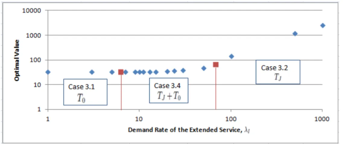
3.5 λP vs Objective Profit when K=100 . . . 40
3.6 λP vs Objective Profit when K=500 . . . 41
4.1 Shipment consolidation operation for only regular service. . . 50
4.2 Model Assumption . . . 56
4.3 Realization . . . 58
4.4 Results of the best combination of (C0, CP) . . . 61
List of Tables
2.1 The separation of cases according to 9 subsets . . . 32
3.1 The experimental parameter set fits BY region. . . 37
3.2 Sets which have only the regular and the joint policy exist . . . 47
3.3 Subset of problems when rP = r0 and λ0 ≤ λP + λ1 . . . 48
3.4 Subset of problems when rP = r0 and λ0 ≤ λP + λ1 with no lost sale for regular service. . . 48
4.1 Parameter set to find best combination between C0 and CP . . . 60
4.2 Parameter set for the comparison between the simulation and the approximate analytical model. . . 62
4.3 Average Inventory Carried (Simulation vs Analytical Model) . . . 62
Chapter 1
Introduction
As the Internet has brought a new channel for communication, many traditional businesses got benefit from it to reach their current and potential customers. Using this new channel not only provided a link to better communication for businesses but also cultivated new ideas about alternative ways of operating them. At the end of 1990s, one of the emerging new business ideas on the Internet was observed in converting traditional retailers into online shops. The basic idea is to carry brick-and-mortar retailing into the Internet by presenting products, making agreements and completing transactions online while keeping some assets such as inventories and distribution systems for physical operations. As a result, the concept of e-retailers (electronic retailers) came into play.
Today, Amazon.com, Alibaba, eBay, Peapod, Etsy, Dell, Walmart.com are some of leading e-retailers. Their customers visit e-shops, choose their items, make transactions via internet and their orders are shipped to them. According to the Forrester Research eCommerce Forecast, online sales are expected to yield $334 billion in 2015 and $480 billion by 2019 in US [1]. Additionally, this pattern for expected increase of sales in e-retailers is also foreseen for many countries. When this is the case, to get bigger slice in the market, e-retailers not only should use the Internet efficiently to provide what customers may want to purchase but also should manage their distribution channels effectively to complete their agreements with their customers. Therefore, today taking a place near the top in the competition of e-retailers depends on both putting high customer expectations and fulfilling them in terms
of physical attributes in their agreements.
One of the key areas of this competition where the e-retailers are battling to beat each other, and perhaps the most significant one, is the promised delivery time. Almost all world wide e-retailers, informs their customers about expected delivery dates and sometimes provides exclusive services such as same-day or two-day shipping. This is such a competitive area that, in 2014, Amazon.com introduced their new patent “Method for Anticipatory Package Shipping” which is basically a method to start delivering items that are anticipated to be purchased by customers [2]. It is a very futuristic idea based on forecasting and has not being applied yet. Of course, one would expect that a powerful inventory and distribution system will be the backbone for its realization. Furthermore, an initial step for such kind of applications is announced in May 2015 and Amazon.com introduced their free same-day delivery option for only a group of items that is exclusively available for the members of “prime service”. When this is the case for Amazon.com, to be able to compete, retailers try to optimize their supply chain operations by opening new warehouses, finding ways to place inventories as close as possible to potential customers, and make use of efficient logistics alternatives.
Directed shipments for an order, though, creates better service levels in terms of the customer satisfaction, they come with very high costs. Moreover, these costs may not be re-flected to customers as the benchmark service level in the market already has high standards. Therefore, managing distribution channels under better utilization of delivery options may result with huge savings in operational costs of e-retailers. We consider a stylized environ-ment with a single product distributed via a single distribution point, say a fulfillenviron-ment center. ”Regular Service” specifies those customer orders within a specified delivery time. The ful-fillment center may ship some products, without an actual order realized, to an inventory location, closer to the location of potential customers and may satisfy a group of customers with a shorter (usually negligible) delivery time. We call this as ”Premium Service”, and the customers of the Premium Service may be a part of the regular customer set, as well as additional customers may be attracted with the more favorable delivery option. The issue of shipment consolidation enters the picture here: How one should plan for a shipment, which consists of products shipped to Regular Service customers, and products shipped to inven-tory for Premium Service customers? We have two constraints: specified promised delivery dates for Regular Service customers should be obeyed, as well as the capacity limitation
of the truck. We introduce other details at the end of the chapter. In this study, we are interested in the cost saving opportunities in terms of shipment activities without exceeding the customer service level which is the maximum length of delivery time.
1.1
Literature Review
In this section, we briefly mention about the related preceding studies in the literature in terms of both their settings and ways of approaching to their solutions.
1.1.1
Background in E-tailing
Basu and Muylle [3] separates an e-commerce activity into five steps: search which is the activity to find products in the web, valuation which is the defining step of possible prices and deciding one of them to buy the item, authentication which is the agreement part between the buyer and the seller, payment where the seller gets the payment, logistics which is the delivering the item physically and lastly support which is the supporting the buyer after sale. The scope of our study is included only in the operations of logistics for e-commerce activities.
Any operation regarding logistics requires a strong distribution network to be able to fulfill expectations of customers. Li and Muckstadt [4] defines an e-retailer’s distribution environment as multi-echelon distribution system. In detail, from central warehouses to regional centers, they may have various types of inventories, all can be considered as customer fulfillment centers. These warehouses also carry various types of products. Therefore, there is not only a direct stream from inventory to customers but also in between warehouses to keep the balance between inventories and be prepared to any possible future demand. Rabinovich and Evers [5] also discusses this problem and tries to provide an insight. Hence, considering inventory balancing in terms of being responsive operationally to any order is also major problem itself in logistics of e-retailers.
order deliveries to customers. De Koster [6] states that it is one of the substantial parts about meeting the expectations of customers. Rabinovich [7] identifies one of the performance measure for inventory management as the ability to satisfying customer expectation with preventing high level of accumulations in inventories. This can be realized with an intelligent warehouse distribution system which provides direct fulfillment of orders to avoid from longer delivery times [6]. Therefore, general attitude towards deciding the right fulfillment center among warehouses for an order is to choose the closest available warehouse to the order destination. Furthermore, today delivery lead times not only has to fulfill the customer expectations, but also be able to compete with other firms. Even if the market still has promised delivery times in days or weeks, e-tailing evolves to promise their customers same-day deliveries. Hence, the importance of quick response to demand increases. However, this short delivery time constraint triggers high shipment costs. Order deliveries can be operated by e-retailers’ own fleet or by third party logistic firms such as UPS, FedEx etc. In either case, the main concern for the e-retailer is to keep its delivery time promise to be able to protect and increase its market share. Thus, sometimes at the expense of high shipment costs, companies are willing to deliver orders in without exceeding the promised delivery time that they indicated to their customers.
Recent studies on e-retailers generally concentrate on inventory allocations to find ways to prevent high shipment costs. Since there is generally an uncorrelated geographical demand and supply distribution in the real world, a wise item allocation to warehouses, at least, may prevent supplying an item from a very distant warehouse with high costs. Xu et al. [8] discusses the order fulfillment decision of an e-retailer company by considering periodic evaluation of customer and fulfillment center assignment and provide a heuristic to minimize costs. Furthermore, Acimovic and Graves [9] points out the shipment decision problem of an e-retailer company by considering inventories located in different regions. They present a heuristic method that considers possible future costs and minimizes current outbound shipment costs. Also, Acimovic and Graves [10] emphasizes replenishment policies and right product allocation problem in inventories or fulfillment centers of an e-retailer company to minimize outbound shipment costs while considering geographical mismatch of supply and demand. On the other hand, Aksen and Altinkemer [11] analyses hybrid brick-and-mortar retailing business in which they have both walk-in and online customers. They consider the problem under classic vehicle routing concept between warehouses and customers. Yanık et
al. [12] carries this approach one step ahead and examines premium products in e-tailers such as groceries that should be delivered within the same day under a multi-vendor environment.
As the literature of e-retailer distribution system concentrates right and practical in-ventory allocation decisions, there is a lack of study on shipment operations to customers. Our interest in logistic operations of e-retailers is the last stage of the distribution system. Specifically, in our study, we focus on the shipment operation between a fulfillment center and customers.
1.1.2
Idea of Shipment Consolidation
Another stream of research that touches our study uses the idea of consolidation. Con-solidation is a strategy in logistics to attain economies of scale in costs per unit carried. The main aim behind the consolidation idea is lowering the cost of individual dispatching by holding items until a predefined threshold. Therefore, consolidation policies may have various characteristics.
Hall [13] classifies consolidation operations in three major groups in terms of physical location: terminal consolidation, vehicle consolidation and inventory consolidation. In the terminal consolidation, items are brought from different locations to be loaded in a temporary terminal and sent via new vehicles to different locations such as cross-docking. On the other hand, vehicle consolidation is defined as a type of milk run and the consolidation is based on collecting and distributing items. Inventory consolidation is basically locating different items in the same place, and dispatching them via a single vehicle. From Hall’s [13]’s definition, shipment consolidation is the combination of concepts regarding inventory and vehicle consolidation: It uses truck’s capacity as an inventory, and releases shipments in the same truck when a threshold is reached. Furthermore, two major groups for cargo types are identified in consolidation strategies by Higginson [14] as common and private carriages. In private carriage, transportation vehicles are operated within the same company, and costs are generally fixed per dispatching operations. On the other hand, if the producer company does not have vehicles and shipment operations are managed by an outside company, the carriage type is considered as common type. In that case, costs my have discount rates according to the agreements between the outside and the producer companies.
The main incentive behind the shipment consolidation idea is to get benefits from economies of scale in per items carried. Higginson [14] states that shipment consolida-tion also increases the control on transportaconsolida-tions by reducing handling operaconsolida-tions of items and resulting more dedicated and direct deliveries. ¨Ulk¨u [15] provides an insight that an-other benefit of consolidation can be observed in environmental issues considering carbon emission. On the other hand, more direct and fast deliveries are achieved generally by in-dividual and expensive shipments. That is why, a shipment consolidation should always consider customer service level. Moreover, some shipment consolidation policies do not only result longer waiting time but also may cause uncertain shipment durations, which is also an another drawback. Additionally, consolidation effects inventory levels and holding costs negatively. Managers may need to find extra spaces or even have to keep larger safety stock caused by uncertain shipment times. As a result, planning and managing a good shipment consolidation policy requires elaborated administrative effort.
Even though, defining a consolidation policy has many dimensions, according to C¸ etinkaya [16] they are separated into two branches in terms of implementation: pure and integrated consolidation policies. The pure consolidation policies include only consolidation decisions without including managerial concerns of other operations. If the extend of a consolidation policy contains a coordination between other operations such as inventory, it is called in-tegrated consolidation policy. Specifically, inin-tegrated inventory and shipment consolidation policies are popular as they are applied by coordinating firms for supply chain operations.
In the literature, there are vast amount of works combining retail activities with ship-ment consolidation ideas. Especially, vendor managed inventories (VMI), which is an agreed operation between a supplier and a business to keep inventory in certain level by providing information about business’ inventory levels, attracts attention in recent years. C¸ etinkaya et al. [17], Axs¨ater [18], C¸ etinkaya and Lee [19], Ching et al. [20], C¸ etinkaya et al. [21], Kutanoglu and Lohiya [22], Mutlu and C¸ etinkaya [23], C¸ apar [24], Kaya et al. [25], ana-lyze shipment consolidation problem under different VMI concepts. Additionally, there exist other retail activities which are studied under the shipment consolidation structure. Hong and Lee [26], Hong et. al. [27] study price dependent demands, where demand is a function of price, under integrated inventory and shipment consolidation activities. Besides, another concept in retail activities that got attention recently is the promised delivery time. It is the length of delivery time that the company guarantees to their customers as promise, and in
some studies it is mentioned as quoted delivery time to customers. ¨Ulk¨u and Bookbinder[28], ¨
Ulk¨u and Bookbinder [29] focus customer sensitivity to promised delivery time in shipment consolidation problems.
Many practical examples regarding shipment consolidation policies exist in literature (Hall [13], Higginson and Bookbinder [30]) Most popular operational rules are quantity-based, time-based and time-and-quantity based policies. Quantity-based policy implies that a ship-ment should be realized when the indicated accumulation of items is reached in terms of quantity or weight. As the load in a shipment is one of the cost determining factor, quantity-based policy have long been take a place in the literature. (as examples see: Jackson [31], Gupta and Bagchi [32], C¸ etinkaya and Bookbinder [33], Hong et al. [27]) On the other hand, time-based policy limits the waiting time to wait the accumulation of items and when the specified duration ends the shipment is realized. (as examples see: Jackson [31], C¸ etinkaya et al. [17], C¸ apar [24]) By limiting the consolidation time length service levels in terms of time are controlled. Lastly, time-and-quantity based or hybrid policy enforces the realization of shipment either when the target load or the specified time limit is reached. (Bookbinder and Higginson [34], Mutlu and C¸ etinkaya [23]) In a hybrid policy, both acceptable service levels and scale economies are considered.
Consolidating shipments received considerable an attention since 1990’s to search for an effective way of operating cargo trucks. Early works generally focus on to find practical jus-tification for shipment consolidation operations. Jackson [31] uses simulation to understand effects of consolidation on holding and fix costs in terms of order volumes and gives an insight about consolidation cycles under time-based, quantity-based and hybrid policies. Burns et al. [35] compares direct shipping operation for each order with the strategy of dispatching orders in a truck in an environment where there is a single supplier and multiple customers located in different regions. They develop an analytical method to minimize the distribu-tion cost that is caused by inventory carrying and transportadistribu-tions. Gupta and Bagchi [32] computes an optimal lot size in a shipment consolidation to minimize cost. All these studies advocate the effectiveness of shipment consolidation in terms of cost minimization. Earlier studies are reviewed by C¸ etinkaya in [16].
Consolidation literature can be reviewed in terms of the demand characteristics consid-ered. There are two main distributions used to describe demand: a distribution that describes
the time between two consecutive customer orders, and another distribution that describes the intensity of a customer order (in other words number of units demanded per order). Markovian structures are employed by several studies [36]. (see examples: Minkoff [37], Higginson and Bookbinder [38], Bookbinder and Higginson [34], Cai et al. [39], C¸ etinkaya et al. [17], C¸ etinkaya et al. [40], Mutlu et al. [41] ) A discrete time Markov Chain represents the demand encountered at each discrete time unit (time between two consecutive customer demand is constant, and intensity of demand at each point is represented by a discrete dis-tribution). A continuous time Markov Process may represent the demand. In that case, the time between two consecutive orders are exponentially distributed random variable. The intensity of demand can be unit (in that case we have Poisson distributed demand) or can be represented by a discrete distribution (in that case we have a compound Poisson distribution with the discrete distribution being the compounding distribution). Specifically, Poisson distributed demand is considered in many studies including: C¸ etinkaya et al. [17], Ching et al. [20], Kutanoglu and Lohiya [22], Hong et al. [27], C¸ apar [24], Mutlu and C¸ etinkaya [23], Mutlu et al. [41], C¸ etinkaya et al. [42], Marklund [43], C¸ etinkaya and Bookbinder [33]. On the other hand, Bookbinder and Higginson [34], Higginson and Bookbinder [38], C¸ etinkaya and Bookbinder [33] and C¸ etinkaya et al. [40] are examples who constructed their problems with compound Poisson distribution.
For dynamic and stochastic shipment consolidation problem, Minkoff [37] considers Markovian approach to model of serving inventories of different customers with various size of vehicles. Higginson and Bookbinder [38] approaches the shipment consolidation problem with discrete-time Markovian Decision Process (MDP) model. In their model, with the ar-rival of each customer the shipper has to make a decision regarding realizing the shipment or not. Their aim is to minimize the cost of per shipment in pure shipment consolidation structure by considering the problem for both private and common carrier. Another study of Bookbinder and Higginson [34] evaluates hybrid policy by using stochastic clearance system under private carrier assumption. Bookbinder et al. [44] considers the problem for private carrier under discrete-time batch Markov arrival process. For an arbitrary time accumu-lated weight of arrived orders in the system and total consolidated weight in a shipment cycle are analyzed and they present a computational method for such performance mea-sures under time-bases, quantity-based and hybrid policies. Cai et al. [39] also employs discrete time batch Markovian arrival process in shipment consolidation problem. In this
study dispatching decision is left as a function in the model. Lastly, Kaya et al. [25] applies MDP in a stochastic environment where a single supplier and a retailer exist by analyzing quantity-based, time-based and hybrid policies.
C¸ etinkaya et al. [17] employs a shipment consolidation problem under renewal theoret-ical model for supplier operating VMI’s. In its setting, the objective is to minimize the expected long run average cost of inventory replenishments under time-based policy by de-ciding both the optimal shipment release interval and the optimal replenishment quantity. An algorithm to calculate exact optimal values for the problem of C¸ etinkaya et al. [17] is provided by Axs¨ater [18]. Later, C¸ etinkaya et al. [40] addresses the problem of [17] with quantity-based consolidation policy having the construction of general compound renewal process for demands. Moreover, C¸ etinkaya et al. [21] compares numerically time-based and quantity-based policies mentioned in C¸ etinkaya et al. [17] and validate that quantity-based policy outperforms in their cost minimization setting. They also propose hybrid policy and provide comparisons with time-based and quantity-based via simulation. Another integrated inventory and transportation problem with similar demand setting to C¸ etinkaya et al. [17] is modeled in multi-facility and single-echelon environment by Kutanoglu and Lohiya [22] under time-based consolidation policy.
Under VMI context in Ching et al. [20] for time-and-quantity-based consolidation policy. It gives closed form version of the optimal solution regarding the sum of the dispatching, the transportation, the inventory and the re-order costs. Furthermore, C¸ etinkaya and Book-binder [33] also considers to apply both time-based and quantity-based shipment consolida-tion policies by covering cost minimizaconsolida-tion objectives for common and private carrier settings separately. They present analytical results for the optimal waiting time for time-based pol-icy and the optimal dispatching quantity for the quantity-based polpol-icy. Even if they assume exponential order weight distribution, their results are applicable for renewal theory setting. Mutlu and C¸ etinkaya [23] focus on finding a solution approach regarding optimal inventory level and outbound shipment scheduling policy parameters under the existence of common carrier costs. They employ time-based and quantity-based dispatching policies and provide a search algorithm for policy parameter for given bounds.
One of the closest study to ours is presented by Mutlu et al. [41] considering pure con-solidation problem with hybrid shipment concon-solidation policy by having Poisson distributed
demand. Their objective is to minimize the total cost which includes expected cost per ship-ment and expected waiting cost of shipship-ment load. The expected shipship-ment cost constitutes fix cost and a loading cost per demand. The capacity of shipment per truck is not incorporated. Furthermore, Mutlu et al. [41] derives an analytical expression for the optimal value of the objective function. They also present an analytical comparison of three shipment policies regarding their performances. On the other hand, C¸ etinkaya et al. [42] focus on the service based comparison of different shipment policies. Order arrivals are distributed as Poisson and they consider maximum waiting time and average order delay as service measures. Their results show that under fixed policy parameters, hybrid policy outperforms the time-based policy in terms of maximum waiting time. Considering the average order delay, again hybrid policy outperforms both quantity based and time based policy separately.
Another stream of VMI concept studies on nonidentical retailers. Marklund [43] analyze an inventory replenishment and shipment consolidation between single supplier and multiple nonidentical retailers. The demand is assumed to be Poisson distributed under time-based dispatching policy. Marklund [43] provides a two heuristic method to to identify expected backorder and holding costs. Furthermore, C¸ apar [24] also use time-based policy to operate shipment activities between an outside supplier, a distribution center and nonidentical re-tailers where each retailer again has Poisson demand. An optimization method to obtain an optimal order-up-to level for retailers and optimal replenishment quantity for the distribution center is provided by them.
Recently, the literature with Poisson demand setting in retail activities is expanded for more complex demand functions: price effecting the demand; quoted delivery time effecting the demand. Hong et al. [27] considered integrated inventory and transportation problem with pricing concern under quantity-based policy. They constructed the model with Renewal theory and analyze the case where demand is a linear function of time. Then, a more general cases such as demand is a concave and convex function of price is presented. Moreover, Hong and Lee [26] employ analysis of optimal time-based consolidation policy by assuming the same relation between demand and price. They present an algorithm to obtain the optimal price, consolidation cycle and replenishment quantity. Their study also includes extensions regarding quantity discounts for dispatching costs and hybrid policy version of the problem. Another case is where demand is affected by the quoted delivery time. ¨Ulk¨u and Bookbinder [28] consider time and price sensitive demand in third party logistics scheme with time based
policy, and extend the study for different pricing schemes. Furthermore, ¨Ulk¨u et al. [29] employ the customer demand that is sensitive to both price and service as delivery time-guarantee. By maximizing the vendors profit, they validate that optimal price is concave for the capacity of the shipment vehicle.
Ultimately, when the shipment consolidation problem has the stochastic demand setting, it can be easily said that one of the main concerns is to wait and accumulate orders. The general attitude towards avoiding the extreme drawbacks from this situation is either incorporating the waiting costs into a cost minimizing objective function or comparing the effectiveness of different shipment policies in terms of expected waiting times or costs as the studies in literature shows.
The second demand class in shipment consolidation problem is the deterministic demand. Even though, most of the recent studies cover the problem for time-based, quantity-based and hybrid policies with stochastic demand settings, there are some recent studies which assumes deterministic demand in retail activities for popular shipment consolidation poli-cies. In C¸ etinkaya and Lee [19], consolidation problem is addressed in third party logistics with deterministic demand. Their main concerns are about frequency of shipments and the critic quantity to replenishing the third party inventories. Thus, C¸ etinkaya and Lee [19] aim is to minimize the total cost and decide the optimal consolidation cycle length within an inventory replenishment cycle. The objective function constitutes four type of costs: in-ventory replenishment, inin-ventory carrying, customer waiting and outbound transportation costs. The capacitated and uncapacitated cargo versions are presented and Karush-Kuhn-Tucker conditions [45] is used to construct enumeration method to reach optimal solution. Later, Moon et al. [46] carry the problem of C¸ etinkaya and Lee [19] a one step further and employ the joint replenishment with multiple items. They introduce two time-based policy and algorithms to reach near optimal parameters for specified policies. Another study using deterministic demand assumption is used by Hwang [47]. In this study, economic lot sizing for transportation, production and inventory decisions is considered with the assumption for stepwise cargo costs.
1.2
Problem Definition
In our study, we combine e-retailer’s environment with shipment consolidation problem under hybrid policy. We assume that the e-retailer has an option to offer two types of delivery services which differ according to their promised delivery times, as well as prices. The offered options are available on the web page when customers navigate in a product. Specifically, when the e-retailer decides to operate a service type for a specific product, customers are able to see only the type of service with promised latest delivery time and price. The first type of service is named as the “Regular Service”. If an item is operated under this service, on the web page customers see a positive maximum length of time that is guaranteed for the item’s delivery. The second type of service is the “Premium Service”. If the e-retailer chooses to operate under the premium service for an item, customers are guaranteed to have immediate delivery when they purchase. In other words, customers are served in negligible amount of time such as shipping in a few hours or at most in the same-day which can be interpreted as zero promised delivery time. Note that, both regular and premium services can be offered at the same time, as well. As a result of the difference in promised delivery times in the premium and the regular services, the demand rates for each service type in each service combination can be different. Thus, the demand rates in different services are represented separately.
Another important issue arising with the idea of zero promised delivery time is the ex-istence of inventories. We assume that the e-retailer has small inventories very close to its demand points such as having small “lockers” in neighborhoods or even a body of shipment vehicle that can serve in zero promised delivery time. The main idea having small inventories is that when the company decides to apply the premium service for an item, they make an anticipated shipment of that item to the vicinity of the demand location and keep inventory to satisfy possible future demand. From the customers’ point of view, if the e-retailer ap-plies this service to an item, customers who are in the same region with such inventories see an immediate delivery option. Hence, this inventory can be considered as a demand point, which actually is a fulfillment center for the premium service customers.
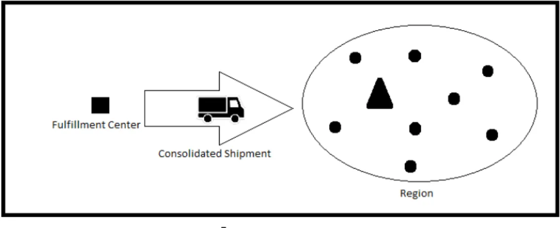
Our problem considers a single echelon structure for the consolidation operation which is between a single fulfillment center and a single customer region. In Figure 1.1 consolidation
activity is represented. In this region, there exist customers and a single inventory point for the premium service. Note that the region is the local area that makes a shipment vehicle serves within a negligible amount of time. When orders come from this region under the regular service, the shipment vehicle waits to consolidate and then ships to the customers in that region. We assume that the time spend within the region for delivery processes and the transportation time between the fulfillment center and the region are both zero without loss of generality. Hence, the shipment vehicle waits in the fulfillment center at most the promised delivery time. On the other hand, it may also carry items which will be offered under the premium service. Therefore, the vehicle consolidates items for both services in a single shipment.
We assume the problem for unlimited fleet availability. However, the shipment vehicle has a constant capacity, another constraint for the problem in addition to the promised delivery time constraint. The problem considers infinite time horizon, hence shipments repeat themselves. Finally, for sake of simplicity, we assume the e-retailer offers a single item to their customers.
The main concerns are to decide how much time a shipment vehicle should wait in a fulfillment center. Note that, by this decision, we implicitly affect two measures: cycle length as the time between two consecutive shipment realizations, and realized capacity of the truck.
We differentiate orders coming in each service in terms of their revenues. Furthermore, each shipment realization has a fixed cost regardless of where it serves: the inventory or customers of the regular service. However, items carried to the inventory causes holding cost per unit per time. Different from literature, we do not include waiting costs to the problem as it is an agreed time length to wait between a customer and the e-retailer. We provide two type of settings for the e-retailer’s consolidation problem. In the first setting, the problem is constructed upon deterministic demand assumption for all type of services, and the model maximizes the average profit. In the deterministic setting, we decide the optimal cycle length by considering different services’ profitabilities. Note that under deterministic demand, finding optimal cycle length corresponds to finding which service (or services) to use within the cycle and their duration. In other words, we allow for one service (or both services together) to stop and another service (or both services together) to start within the cycle, if it is profitable. In the second setting, we first assume that the e-retailer excludes the premium service option and operates only the regular service which has Poisson distributed demand under hybrid consolidation policy, similar with Mutlu et al. [41]. However, different then Mutlu et al. [41] we have only fixed cost per shipment as pure consolidation prob-lem, and the model maximizes expected profit. Then, we extend the problem by including the premium service option having a constant deterministic demand rate, and provide an approximate model. In the extended problem,the model maximizes the expected profit by deciding optimal amount to send the inventory for the premium service, serving the regular customers under hybrid consolidation policy.
The rest of the thesis includes is as follows. In the next chapter, we present the shipment consolidation problem for an e-retailer under deterministic demand. We present analytical results and a solution methodology to determine an optimal solution. In Chapter 3, a continuum of Chapter 2, we provide numerical results and analyze special cases. In Chapter 4, we address the shipment consolidation problem of e-retailer under stochastic demand structure, specifically we assume that the regular services’ demand follows a Poisson process and we analyze two cases. The first case, when there is no possibility for the premium service, we evaluate hybrid (time-and-quantity) shipment consolidation policy for the regular service operation. In the second case, we assume that additional to the regular service, we have the premium service possibility to serve customers with deterministic demand. We propose a simple policy.. policy. Note that when demand is stochastic, we can only optimize the
decisions with respect to a stated policy, unlike like deterministic demand case, where we were able to find the optimal policy (which allows the use a combination of services within a cycle, so long objective function is maximized). We evaluate an approximate analytical model to optimize the policy proposed and evaluate the approximation with simulation. In the last chapter, we conclude our study by summarizing our results and offering possible extensions.
Chapter 2
Shipment Consolidation Problem of
E-tailing with Deterministic Demand
2.1
Model Description
In this chapter we consider a deterministic constant demand environment. Particularly, we assume the demand rate for the regular service customers to be constant and known, as well as the premium service. We assume an infinite horizon problem, resulting in finding shipment cycles which will repeat. Hence, the objective function can be specified as maximization of average contribution, contribution meaning as revenues minus costs. For simplicity, we assume that each order comes as a single unit. Under above constructions, we investigate different operational strategies for the e-retailer.
Note that shipment consolidation for this case means that we would like to include the orders for the regular service customers, as well as the products that are moved to closer inventory location for the prospective premium service customers. We allow for possible lost sales for both types of customers. Hence the decision problem is to find a shipment cycle. Note that within a shipment cycle, there will be a single shipment, part of the products in this shipment will be used to satisfy orders (regular service) and the remaining will be inventoried to satisfy premium service customers. The costs associated with this decision
are a fixed cost of transportation and inventory carrying cost for the inventoried products. The revenue associated with the decision is the revenue obtained from sales of both type of customers. Note that loss of revenue can be defined as cost of lost sales, as well. The contribution obtained for the duration of the cycle is then divided by the cycle length to find the average contribution.
Finally, we define the cycle length in terms of three decision variables: T0, total duration
within the cycle where we only aim to satisfy regular service customers; TP, total duration
within the cycle where we only satisfy premium service customers; TJ, total duration within
the cycle where we satisfy regular service, as well as premium service customers at the same time. These three durations can be considered to represent three different operational strategies. We analyze these strategies in detail.
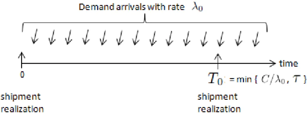
The first operational strategy is to apply “regular policy”. In this policy, the company quotes a delivery time to its customers and delivers them in the quoted amount of time. Hence, TQ based policy has a defining role on the cycle length of shipments. The relation between the regular policy’s demand rate and time length of two consecutive shipments is shown in Figure 2.1.
Figure 2.1: The Regular Policy
where
λ0: the demand rate of regular service
τ : the promised delivery time C : capacity of the shipment truck
T0: total duration within the cycle length where only the regular service exists.
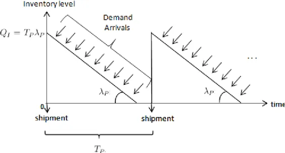
The second operational strategy for deliveries of the e-retailer company is what we call “premium policy”. Being different from the regular policy, in this operation rule, the com-pany keeps a close inventory for its customers. This inventory ensures that the comcom-pany can deliver customers’ orders in a very short amount of time such as within the same day or even within a few hours after customers give their orders. In that case, the promised delivery time is not the concern of the company’s service quality. Thus, this policy can be considered as an exclusive service for committed or loyal customers, as well. As all orders are fulfilled from this “closest” inventory, a shipment, in this case is to the location of inventory before demand is realized. Hence, the only limitation for the cycle length of a shipment is the capacity of vehicle. In Figure 2.2, the relation between the inventory level and the time between two consecutive shipment is demonstrated. Notice that each shipment can be considered to feed next cycle’s demand as customers are assumed to be satisfied from the inventory. Here, we show the demand rate for the premium service as an inventory that decreases with demand.
Figure 2.2: The Premium Policy
λP: demand rate of the premium service
TP: total duration within the cycle length where only the premium service exists
QI: the beginning inventory level (assumed to be delivered at the end of each cycle).
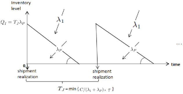
As a final operational strategy, the regular and the premium policies are considered to-gether and called the joint policy. In this operation option, the company leaves the delivery choice to its customers by offering the regular and the premium service options at the same time. In other words, customers see two type of delivery options with different promised delivery times for the item. Since the decision is made by customers, the total demand of the joint policy are fed by two streams according to customers’ choices. At this point, it is assumed that having two types of service option at the same time will affect the demand rate coming from regular customers. Hence, the demand rate of regular service users in the joint policy is different from the demand rate of the regular policy, λ0. The intuition would be
a decreasing demand rate for regular service, when both are offered. However, we allow for more general structures and do not restrict the demand rate in this case. Furthermore, as the joint policy has the premium service option, it also uses the inventory. In the same man-ner, for customers who choose the regular service option, the joint policy takes the promised delivery time into account. Notice that, the capacity limitation of a single shipment which serves regular customers and the inventory is still valid. Additionally, under the joint policy, we do not allow lost sales from neither the regular nor the premium delivery service as both services are available to the customers. In Figure 2.3, the relation of inventory levels and the cycle length considering demand rates can be seen.
Figure 2.3: The Joint Policy
where
λ1: demand rate of regular service customers in the joint policy
TJ: total duration within the cycle length where only the joint policy exists.
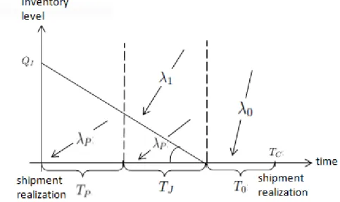
Ultimately, to be able to make a comparison between all policies, we consider all of them at the same time. As it can be seen in Figure 2.4, the cycle length is constituted by the sum of time lengths devoted to each policy. Therefore, deciding contributions of T0, TP and TJ to
the cycle length leads us to the optimal policy selection if we consider all policies together in the same deterministic setting problem. From the customers point of the meaning of the cycle length is the following: When the shipment is realized and TP is positive, customers
can see only the premium service option to purchase the item with zero promised delivery time which is provided by keeping the items in the close inventory. In the same manner, when customers visit the web page of the item in TJ parts of the shipment cycle, they see
both types of delivery option available and they decide according to their wishes. Lastly, if the web page of the item is visited in T0 portion of the cycle, customers has only regular
service option for the item’s delivery. Notice that, if the cycle length has only positive TP,
only T0 in the cycle length means lost sale from customers of the premium service.
Figure 2.4: The Regular, The Premium and The Joint Policies
where
TC: the cycle length.
Regarding different delivery strategies that the company can operate, the revenue per unit is denoted separately for different demand types. Also, the total revenue coming from each policy option is calculated and divided by the cycle time as the problem takes place in the infinite horizon. First of all, the total revenue of the regular policy per cycle time is expressed.
T0 ∗ r0 ∗ λ0
TP + TJ + T0
where r0 is the revenue in regular service policy for per unit.
Accordingly, the revenue per cycle time generated by the premium service policy is shown as follows.
TP ∗ rP ∗ λP
TP + TJ + T0
where rP is the revenue per unit of the premium service.
The joint policy leaves the delivery decision to customers of the company by offering both the regular and the premium delivery options at the same time. For customers who prefer the regular delivery service in the joint policy, the revenue per unit is taken as the same with the regular policy’s revenue per unit. In the same manner, customers who prefer the premium delivery option when the company operates according to the joint policy, the revenue per unit of premium service is taken same with the revenue per unit of extend policy. To calculate the joint policy’s revenue per cycle time, the revenue coming from each stream of shipment type is accounted and represented as can be shown below.
TJ ∗ (r0∗ λ1+ rP ∗ λP)
TP + TJ + T0
In the model, there are two types of operational costs: the inventory and shipment related costs. First of all, it is assumed that for each shipment and respectively for each cycle time, there is a fixed cost to pay. In our problem, the fix cost is the same for each shipment cycle and expressed as follows.
K TP + TJ + T0
where K is the fixed cost per shipment.
The second cost component is inventory related costs. The inventory related cost is taken as the holding costs for each unit per time. Since both the joint and the premium service policies use the inventory, the inventory cost function takes the time spend on premium
service and the time spend on joint service as its two variables. Hence, the inventory cost per cycle time can be shown as:
H(TP, TJ)
TP + TJ + T0
where H(TP, TJ) is the inventory cost function.
The inventory cost function, H(TP, TJ), is taken as a linear function of time. h0 is
con-sidered as the holding cost per unit per time and the expression for the inventory cost per cycle time becomes:
h ∗ λP ∗ (TP + TJ)2
TP + TJ + T0
where h = h0/2.
In the problem of deciding the right operation rule for the e-commerce company, our objective is to maximize the total contribution to profit. As a result, the objective function of the problem is taken as the total revenue per cycle time subtracted from the total revenue per cycle time. The final form of the objective function is expressed as follows.
TP ∗ rP ∗ λP + TJ ∗ (rP ∗ λP + r0∗ λ1) + T0∗ r0∗ λ0− K − H(TP, TJ)
TP + TJ + T0
where
H(TP, TJ) = h ∗ λP ∗ (TP + TJ)2.
However, there are two important considerations for the admissibility of model regarding the capacity of a shipment and the promised delivery time. The constraint that ensures serving to customers in the promised delivery time considers only customers who use regular
delivery option as it is assumed that customers of the premium delivery get their orders immediately from the inventory. Therefore, the promised delivery time is a bound for the regular delivery service which exists in the operation rule of both the joint and the regular policy. Explicitly, the sum of time durations of these two policies should be less than or equal to the promised delivery time and it can be shown below.
T0+ TJ ≤ τ
where τ is the promised delivery time.
Secondly, in each cycle, a shipping vehicle serves with its constant capacity and carries all customer demands regardless of their types. Therefore, the capacity limit of the vehicle is filled in the regular policy duration with the regular service demand, in the premium policy duration with the premium service demand and in the joint policy duration with its premium and regular services’ demand. The constraint belonging to the capacity consideration of the shipment vehicle is expressed as follows.
TP ∗ λP + TJ∗ (λP + λ1) + T0∗ λ0 ≤ C
where C is the capacity of a shipment.
Finally, variables of the problem cannot be negative since time lengths cannot be negative.
TP, TJ, T0 ≥ 0
2.2
The Model
The complete form of the model is as follows.
rP: revenue per unit of the premium service
r0: revenue per unit of the regular service
λP: demand rate of the premium service
λ1: demand rate of regular service customers in the joint policy
λ0: demand rate of regular service
h: inventory holding cost K : fixed cost of a shipment τ : promised delivery time C : capacity
Variables:
TP: time length used in the premium policy
TJ: time length used in the joint policy
T0: time length used in the regular policy
Maximize TP ∗ rP ∗ λP + TJ ∗ (rP ∗ λP + r0∗ λ1) + T0∗ r0∗ λ0− K − H(TP, TJ) (TP + TJ+ T0) (2.1) subject to T0+ TJ ≤ τ (2.2) TP ∗ λP + TJ ∗ (λP + λ1) + T0∗ λ0 ≤ C (2.3) TP, TJ, T0 ≥ 0 (2.4) where H(TP, TJ) = h ∗ λP ∗ (TP + TJ)2 (2.5)
2.3
Analysis of the Model and the Optimality
Condi-tions
The objective function, (2.1), has a nonlinear structure. It is neither concave nor convex. See the examples in Appendix A. Hence, it is not possible to use sufficient conditions of Karush-Khun-Tucker (KKT) to reach the global optimal solution [45]. On the other hand, constraints and the objective function of the model satisfy requirements for KKT to be used as necessary conditions. Hence, it is possible to explicitly evaluate all solutions of the problem indicated the necessary conditions and choose the one that yields the maximum value for the objective function. Notice that, the necessary KKT conditions do not guarantee to get a positive objective value in the optimal solution. As values of cost variables change, the sign of the objective value may change. Hence, the necessary KKT conditions yield positive or negative solutions as the optimal value.
To obtain the necessary KKT conditions, we need the Lagrangian function form of the problem. We define µ1 and µ2 as the Lagrangian multipliers of the promised delivery time
constraint (2.2) and the capacity constraint (2.3), respectively. Under these constructions, the Lagrangian function of the problem is formed.
L(TP, TJ, T0, µ1, µ2) = f (TP, TJ, T0) + µ1∗ g1(TJ, T0) + µ2∗ g2(TP, TJ, T0) (2.6) where f (TP, TJ, T0) = TPrPλP + TJ(rPλP + r0λ1) + T0r0λ0− K − hλP(TP + TJ)2 TP + TJ+ T0 (2.7) g1(TJ, T0) = T0+ TJ − τ (2.8) g2(TP, TJ, T0) = TPλP + TJ(λP + λ1) + T0λ0− C (2.9) µ1 ≥ 0 (2.10) µ2 ≥ 0. (2.11)
Finally, we are able to construct KKT conditions to find each possible solution of the problem.
Stationarity: ∂L ∂T0 = 0 (or ≤ 0 if T0∗ = 0) (2.12) ∂L ∂TP = 0 (or ≤ 0 if TP∗ = 0) (2.13) ∂L ∂TJ = 0 (or ≤ 0 if TJ∗ = 0) (2.14) Primal Feasibility: g1(TJ, T0) ≤ 0 (2.15) g2(TP, TJ, T0) ≤ 0 (2.16) TP, TJ, T0 ≥ 0 (2.17) Dual Feasibility: µ1 ≥ 0 (2.18) µ2 ≥ 0 (2.19) Complementary Slackness: µ1∗ g1(TJ, T0) = 0 (2.20) µ2∗ g2(TP, TJ, T0) = 0 (2.21)
After defining the necessary KKT conditions of the problem, we evaluate each of them to be able to generate all possible solutions. Cases are created according to the domain of each variable of the Lagrange function (2.6). More explicitly, a case can take a value of a variable either equal to zero or greater than zero. In the model, two possible options for subsets of three original variables and two Lagrange multipliers are shown in (2.22), (2.23), (2.24), (2.25) and (2.26) and they generate 25 = 32 different cases for our model.
T0 = 0 or T0 > 0 (2.22) TJ = 0 or TJ > 0 (2.23) TP = 0 or TP > 0 (2.24) µ1 = 0 or µ1 > 0 (2.25) µ2 = 0 or µ2 > 0 (2.26)
2.4
Analysis of KKT Conditions
By obtaining 32 cases of the main problem, we have all required equalities for each case that the necessary KKT conditions yield. Each case is solved with corresponding KKT conditions valid for the case. Solutions and related derivations are in Appendix B. Our analyses on 32 cases reveal that some case are not meaningful in terms of the problem considered. The following observations and a proposition are used to identify those situations.
Notice that cases that yield ”no operation” option are eliminated from further consider-ation. Of course, if the problem parameters require no economical operation (this means that we have negative contribution to profit if operation is forced) these cases would be important. Nevertheless we can always depict such situations once the problem solution is obtained.
Observation 1: There exist some cases with solutions requiring problem parameters to attain unrealistic values. Hence, these cases are eliminated from further consideration. Please refer Appendix B for indicated cases.
1. Case 4.1 is infeasible since its solution, (T0, TJ, TP) = (∞, 0, 0), is only possible when
K = ∞.
2. Cases 1.3 and 2.3 that are constructed by µ1 > 0 with T0 = 0 and TJ = 0 are not
ad-missible as this structure forces the first inequality to be zero. However, the promised delivery time, τ , cannot be zero.
Observation 2: There exist some cases with solutions requiring trivial relations to hold among parameters. Hence, these cases are eliminated from further consideration unless the parameter values are such that the mentioned trivial relations hold. Please see Appendix B.
1. Since Case 1.1 is in the intersection of Case 2.1 and Case 3.1, Case 1.1 is feasible if and only if C = λ0τ .
2. Since Case 1.2 is in the intersection of Case 2.2 and Case 3.2, Case 1.2 is feasible if and only if C = (λP + λ1)τ .
3. Case 4.3, Case 4.6 and Case 4.7 are feasible if and only if r0λ1 = 0.
4. Case 4.4 is a special version of Case 4.2 and it is feasible if and only if K =
(rPλP+ r0λ1− r0λ0)2
4hλP with having T0 = 0.
5. Case 4.5 is a special version of Case 4.3 and it is feasible if and only if K = (rPλP− r0λ0)2
4hλP
with having TJ = 0.
Observation 3: There exists some cases with solutions forcing the decision variables to take values that are also admissible within the range of another case. Hence these cases are eliminated from further consideration. For such cases please see following cases in Appendix B.
1. Case 3.7 converges Case 3.4 as its solution forces TP to be zero.
2. Case 4.6 converges Case 4.3 as its solution forces TJ to be zero.
3. Case 4.7 converges Case 4.5 as its solution forces TJ and T0 to be zero.
Proposition 1. If two cases take their values of parameters from the same set, then the case with a larger feasible region yields the same or a better objective value. Hence, if two such cases are feasible given a parameter set, the case having a larger feasible area dominates
the other. In the following list, we show some of such cases and for the others please refer Appendix C. Let, Oi be the objective value of case i and Fi be the feasible region of case i.
i. O1.1 ≤ O2.1 since F1.1 ⊆ F2.1 ii. O1.1 ≤ O3.1 since F1.1 ⊆ F3.1 iii. O1.2 ≤ O2.2 since F1.2 ⊆ F2.2 iv. O1.2 ≤ O3.2 since F1.2 ⊆ F3.2 v. O1.3 ≤ O2.3 since F1.3 ⊆ F2.3 vi. O1.3 ≤ O3.3 since F1.3 ⊆ F3.3.
2.5
Solution
After solving the problem with necessary KKT conditions and eliminating redundant cases, we further investigate each case with respect to the cost parameters K and h. For most of the cases, we are able to detect bounds for K and h from the inequalities originated by (2.12), (2.13) and (2.14). On the other hand, for other cases finding neat expressions is impossible due to complexities of inequalities. For generated bounds of K and h please refer to Appendix D. These bounds are interpreted as the value limits of related cost parameters and outside these bounds, cases are not admissible.
Observation 4: There exist economical limitations for cases to operate, which are different from the original feasible conditions. These limitations are generated from their stationary KKT conditions. If for a case with given parameter set, its stationary conditions do not hold, it is eliminated from the possible solutions. For some cases, these economical conditions are simplified to obtain neat cost bounds for K and h. Such cases and their cost bounds are presented in Appendix D.
2.5.1
The Solution Framework
We observe that bounds generated for K and h contain similar expressions for marginal rev-enues and demand rates in almost all remaining cases. Therefore, we further expose these cases by looking at expressions of marginal revenues and demand rates that they have in their K or h bounds. We use these expressions as a framework which enables us to under-stand the environment and the behavior of the problem in terms of demand and revenue relations between different policies. Therefore, according to the demand relations, we divide the problem into three mutually exclusive subsets in terms of demand rates.
• X : λP ≥ λ0 where the demand rate of regular service is not greater than the demand
rate of the premium service.
• Y : λP + λ1 ≥ λ0 and λP ≤ λ0 where the demand of only premium service is less than
the demand of regular service. Yet, the total demand rate of joint policy is greater than or equal to the demand of regular service.
• Z : λ0 ≥ λP + λ1 where the demand of regular service is greater than or equal to the
total demand rate of the joint policy.
To address more plausible division of subsets we also consider relations of different de-mand rates with respect to their revenues generated per unit time. As a result, we reach three subsets.
• A: rPλP ≥ r0λ0 where the total revenue of the premium policy is greater than or equal
to the revenue coming from the regular policy.
• B : rPλP+ r0λ1 ≥ r0λ0 and rPλP ≤ r0λ0 where the revenue generated from joint policy
revenue of premium policy is not greater than the revenue of regular policy.
• C : r0λ0 ≥ rPλP + r0λ1 where the total revenue coming from regular policy is greater
than or equal to the revenue originated from the joint policy.
2.5.2
The Analysis of Model Subsets
We have three subsets for demand rates and three subsets for total revenues per unit time. With the combination of A,B,C and X,Y,Z, the problem environment is divided into nine distinct subsets: AX,AY,AZ, BX,BY,BZ, CX,CY,CZ. To find the subset(s) where each of remaining 17 cases is able to survive, both feasibility of Lagrange multipliers and econom-ical conditions mentioned in Observation 4 are considered in terms of bounds that we find for K and h. Notice that cases which are feasible only when a special relation holds be-tween parameters or cases which converge to other cases are not included. Consequently, the categorization of each case is shown in Table 2.1. For details please refer to Appendix E.1.
X Y Z 1.4, 1.5, 1.6, 1.7, 1.4, 1.5, 1.6, 1.7, 1.4, 1.5, 1.6, 1.7, A 2.2, 2.4, 2.5, 2.6, 2.7, 2.2, 2.4, 2.5, 2.6, 2.7, 2.2, 2.4, 2.5, 2.6, 2.7, 3.1, 3.2, 3.3, 3.4, 3.5, 3.6, 4.2 3.2, 3.3, 3.4, 3.5, 3.6, 4.2 3.2, 3.3, 3.5, 3.6, 4.2 1.4, 1.6, 1.7, 1.4, 1.5, 1.6, 1.7, 1.4, 1.5, 1.6, 1.7, B 2.1, 2.2, 2.4, 2.5, 2.6, 2.7, 2.1, 2.2, 2.4, 2.5, 2.6, 2.7, 2.1, 2.2, 2.4, 2.5, 2.6, 2.7, 3.2, 3.4, 3.6, 4.2 3.1, 3.2, 3.3, 3.4, 3.5, 3.6, 4.2 3.2, 3.3, 3.5, 3.6, 4.2 1.6, 1.5, 1.6, 1.4, 1.5, 1.6, 1.7 C 2.1, 2.5, 2.6, 2.1, 2.5, 2.6, 2.1, 2.5, 2.6, 3.4, 3.6 3.3, 3.4, 3.5, 3.6 3.1, 3.2, 3.3, 3.4, 3.5, 3.6
Table 2.1: The separation of cases according to 9 subsets
As each subset of the problem has different characterization regarding demand rates and total revenues per unit time, cases in a single subset are analyzed separately from cases of
other subsets. There exist intervals for K or h such that some cases are not admissible at the same time and these value intervals can be ordered consecutively. For explicit relations please refer to Appendix E.2. Therefore, values of K or h alter the case which yield feasible solution to us. Unfortunately, we cannot order relations for regarding K or h for all subsets. However, these ordered relations help us to decrease the number of possibilities which we search for the optimal solution.
Observation 5: There exist global orders of cases that are valid in all nine sets in terms of their K intervals which are defined by lower and upper bounds of K. Please see Appendix E for the detailed ordering. Let Ki be the minimum K value that makes the case i feasible and respectively Ki is the maximum value of K which makes case i feasible. We define Ki
as the interval defined by [Ki, Ki] for case i. An order for cases i,j Ki ≤ Kj means that
Ki ≤ Kj. Note that same notation for cost parameter h is also valid, such ordered cases are
as follows.
1. K2.1 ≤ K2.5
2. K4.2 ≤ K2.2 ≤ K2.6
3. K4.2 ≤ K3.2 ≤ K3.6 ≤ K3.3 ≤ K3.5
4. h1.4 ≤ h2.4 - except AZ and BZ subsets
The significance of these divisions of the problem set comes from its ability to differentiate the products. For example, if a product has aspects that match one of the nine combinations, then there are actually less candidates for the optimal policy. Hence, the solution structure may change with products which have different demand and revenue per unit characteristics.
2.5.3
Solution Algorithm
The model satisfies only necessary conditions of KKT. Hence, the solution algorithm should be based on finding all feasible cases and selecting the feasible case that yields the highest
optimal value. Our solution algorithm is constructed on nine sets and ordered intervals of K and h as mentioned in Observation 5.
Initially, the algorithm checks each special case which have special equations to be admis-sible as in Observation 2 and 3. If feasibility conditions hold, the solution algorithm adds it to the Candidate List. Else, it writes down the condition(s) which violates its feasibility.
When the algorithm finishes the check of special cases, it finds the subset that the problem belongs by using values of demand and revenue per unit parameters. Subsequently, the algorithm directs itself only this subset and considers only cases of this subset. At this point, the algorithm starts to check which interval K and h fall by using the information given in Observation 5. Each ordered relation provides at most one candidate and if the algorithm has one candidate, it checks its feasibility. By controlling all ordered relation lists of this subset and cases that are not belong such ordering in the subset, the algorithm updates the Candidate List. When the check finishes, the algorithm calculates optimal values of each member of the Candidate List. Consequently, it gives the highest value as the optimal solution. Of course, it is easy to check if there are any alternative optimal solutions. In the following Algorithm 1, the pseudo code of algorithm is presented.