D O I: 1 0 .1 5 0 1 / C o m m u a 1 _ 0 0 0 0 0 0 0 7 3 7 IS S N 1 3 0 3 –5 9 9 1
AN ECONOMETRIC APPROACH TO TOURISM DEMAND: EVIDENCE FROM TURKEY
MEHMET YILMAZ AND BUSE BÜYÜM
Abstract. This study focuses on modelling tourism demand with using num-ber of tourists who came to Turkey between the years 1966-2012 (47 years) and bed numbers belonging to accommodation facilities with tourism opera-tion licensed. The number of tourists and beds have only been reached dealing with the years 1966-2012. Except from these variables, many variables such as states investment incentives on tourism, tourism revenues, the annual average temperature, the parity of foreign currency like Euro, dollar and power of pur-chasing in the country could be taken into account. The aim of this paper is to create a forecasting model about the number of coming tourists and to provide prior information for tourism policies by regarding introduced models. In this sense, forecasting of international tourist arrivals for 2013-2020 is purposed.
1. Introduction
Turkey’s tourism development process shows a signi…cant improvement especially after 1980 and “Tourism Encouragement Law” which was enacted in 1982 was a turning point for this development. Increasing number of tourists with encour-agement provided in Turkey’s tourism sector has increased tourism revenue and had a considerable amount in countries’ income. By providing of encouragement measures, bed numbers which belong to accommodation facilities with tourism op-eration licensed rose to 325.168 from 56.044 between 1980 and 2000 and in this process the number of tourists increased to 10.412.000 to 1.288.000 with eight-fold increase. The end of 2012 the number of beds increased to 715.692 and the number of tourists is also 31.782.832. ([10].)
Because the developments in the tourism sector is very important for many countries in order to forecast the number of tourists is vital importance to plan investment in this sector and for touristic businesses who wants to better prepare themselves for the next year. In order to determine a forecasting model on the basis of countries the factors such as the countries’geographical location, the situation of social, political
Received by the editors: October 10, 2015, Accepted: November 25, 2015.
2010 Mathematics Subject Classi…cation. Primary 37M10, 62M10; Secondary 91B84. Key words and phrases. Tourism demand, tourism demand modelling, forecasting, inverse models, time series models, exponential smoothing models.
c 2 0 1 5 A n ka ra U n ive rsity 99
and technological, the width of countries’ seasonal range and the e¢ cient use of resources season by season, the cultural and historical richness should be taken into consideration. In addition to these factors, the countries’advertising network, the distance to other countries, the relative exchange rates [2], the presence of tourism promotion, the number of tourism companies and the number of tourist facilities with tourism operation licensed and the capacity of beds are also important elements for the number of tourists arriving in the country.
For nearly 30 years, researches have proposed regression models with parametric and non-parametric methods modelling and forecasting the tourism demand. It is found that over 130 studies which are scanned index are related to tourism de-mand and forecasting this dede-mand since 2000. Usually in these studies linear and nonlinear dynamic models (Autoregressive (AR)), Autoregressive Integrated Mov-ing Average (ARIMA) and seasonal autoregressive (SAR) are used [8]. Because tourism revenue keep a signi…cant place in countries with a wealth of tourist at-tractions, modeling the number of tourists and tourism income on the basis of countries is important. For example [9] have proposed both static and dynamic models in their studies with variables such as capita national income of tourists and the Money they spend etc. For modelling the number of tourists who arrived to Hong Kong. [3] has combined linear and nonlinear models to forecast tourism demand. [4] has mentioned a detailed compilation of some of the works done so far for prediction model.
In this study, forecasting of the number of tourists has been purposed with using number of tourists who came to Turkey and number of beds which belong to ac-commodation facilities with tourism operation licensed in 1966-2012. Because the number of beds isn’t known on the forecasting period, time series and exponential smoothing model suggestions have been studied to forecast these numbers. Accord-ing to basic economic law, the service has a certain threshold point and however how much the service increases after this point, the number of tourists will reach a saturation point. In the literature the models which test this law are called as inverse models. In this study, reverse models have been handled …rstly and in ad-dition to these mixture models have been proposed. In these models, the models with econometric problems have been examined. Finally the number of tourists who may come to Turkey between the years of 2013-2020 have been forecasted with determining the model used in forecasting by computing RM SE values with ex-post forecasting.
2. Model Suggestions
Primarily, variables such as “number of beds for tourism operation certi…ed resorts” and “the number of foreign tourists” have been plotted in a scatter plot by using IBM SPSS 2.0 software package. On this chart curve …tting options have ‡agged as linear, quadratic, cubic, logarithmic etc. and then the analysis has been conducted. As a result of this analysis the following 10 models have been proposed in the …rst
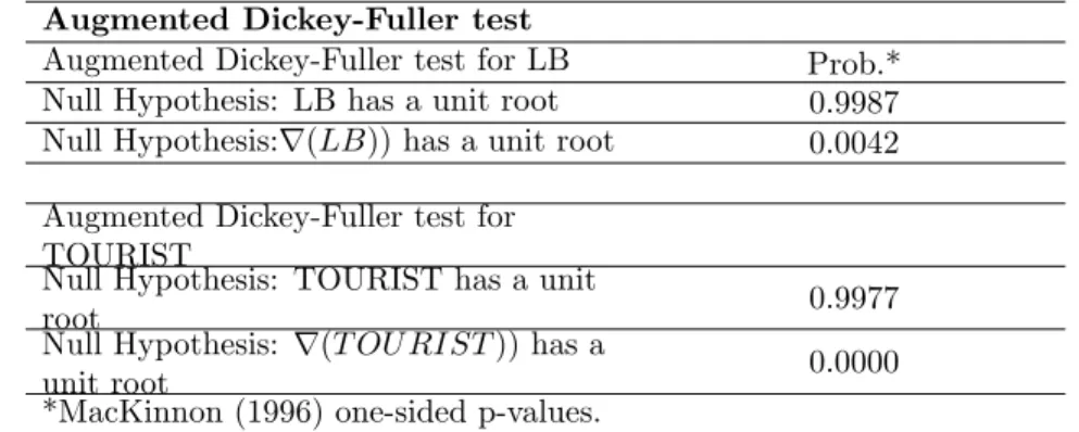
Table 1. Augmented Dickey-Fuller tests and Johansen Cointegration Test of LB and TOURIST
Augmented Dickey-Fuller test
Augmented Dickey-Fuller test for LB Prob.*
Null Hypothesis: LB has a unit root 0.9987
Null Hypothesis:r(LB)) has a unit root 0.0042 Augmented Dickey-Fuller test for
TOURIST
Null Hypothesis: TOURIST has a unit
root 0.9977
Null Hypothesis: r(T OURIST )) has a
unit root 0.0000
*MacKinnon (1996) one-sided p-values.
Unrestricted Cointegration Rank Test (Trace)
Hypothesized Trace 0.05
No. Of
CE(s) Eigenvalue Statistic
Critical
Value Prob.**
None * 0.251739 17.22511 25.87211 0.3983
At most 1 * 0.088603 4.174947 12.51798 0.7167
Trace test indicates no cointegration at the 0.05 level * denotes rejection of the hypothesis at the 0.05 level **MacKinnon-Haug-Michelis (1999) p-values
place by using E-views 6.0 package program. During making these proposals the models which have a high percentage of explanation (R2) is based on by ignoring assumptions of the error terms. Because of encountering di¤erent information cri-teria despite the high value of R2 whether it is a spurious regression relationships between T OU RIST and LB variables have been investigated. For this investiga-tion …rstly unit root test has been made and then the cointegrainvestiga-tion test has been applied (see Table1). In Augmented Dickey Fuller Test (ADF) options of trend and constant term have been marked and it is found that both T OU RIST and LB have one unit root.
As it can be seen that there is no cointegration and there is no coexistence for these two variables that act behavior against time, so it can be said that there isn’t any spurious relationship. In order to see that long term e¤ects of these two variables on each other, the variance decomposition of the …rst di¤erences has been made. The purpose of variance decomposition is to show that the e¤ect of random shocks on the variables. Calculating the explanation rate of the shocks on a variable by the other variables will provide a better understanding of economic relations between variables.
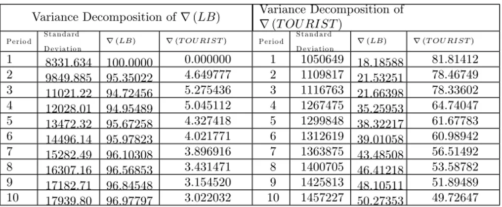
Table 2. Variance Decomposition of r(LB) and r(TOURIST)
Variance Decomposition of r (LB) Variance Decomposition ofr (T OURIST ) P e rio d S t a n d a rd D e v ia t io n r (LB) r (T OURIST ) P e rio d S t a n d a rd D e v ia tio n r (LB) r (T OURIST ) 1 8331.634 100.0000 0.000000 1 1050649 18.18588 81.81412 2 9849.885 95.35022 4.649777 2 1109817 21.53251 78.46749 3 11021.22 94.72456 5.275436 3 1116763 21.66398 78.33602 4 12028.01 94.95489 5.045112 4 1267475 35.25953 64.74047 5 13472.32 95.67258 4.327418 5 1299848 38.32217 61.67783 6 14496.14 95.97823 4.021771 6 1312619 39.01058 60.98942 7 15282.49 96.10308 3.896916 7 1363875 43.48508 56.51492 8 16307.16 96.56853 3.431471 8 1400705 46.41218 53.58782 9 17182.71 96.84548 3.154520 9 1425813 48.10511 51.89489 10 17939.80 96.97797 3.022032 10 1457227 50.27353 49.72647
It can be said that at the end of 10thperiod, 97% of e¤ect of unit shock on r(LB) can be explained by itself. r(T OURIST ) can explain approximately 80% of the e¤ect of the shock by itself in the …rst period, this rate has declined to 50% at the end of the period. The number of beds is not impressed by the number of tourists in long term so it is more related to the value in the previous periods. The reason for this can be economic shocks such as tourism promotion in 1982, terror attacks in the 90s and restricting the promotion that provided to the tourism sector since 1992 etc. It can be said that considering the variance decomposition for the number of tourists, the e¤ect may be associated with number of beds in long term and the number of tourists cannot be a¤ected as much as the number of beds regarding with the experienced economic shocks.
According to these, the models (linear, logarithmic and inverse) where T OU RIST is described only with LB are given in Table 3; the models which are explained by LOG(LB) and time trend are given in Table 4; the dynamic models which include the lagged value of LOG(T OU RIST ) and a mixture of LOG(LB) and time trend are given in Table 5. Also in these tables, the value of R2and AIC and the results of model assumptions are given.
Table 3. Proposed Linear, Logarithmic and Inverse Models by Ignoring Assumptions on Residuals M O D E L R2 A IC H e t e ro s c e d a s -t ic ity ( W h ite Te s t) p va lu e A u to -C o rre la tio n ( B re u s ch -G o d fre y Te s t) p va lu e N o rm a lity ( J a rq u e B e rra ) p va lu e 1 LOG(T OU RISTt) = 0+ 1LOG (LBt) + t 0 .9 8 4 -0 .7 3 2 0 .2 6 3 0 .0 0 0 0 .4 1 6 2 LOG(T OU RISTt) = 0+ 1 1 LOG(LBt)+t 0 .9 6 6 -0 .0 1 4 0 .0 0 3 0 .0 0 0 0 .2 8 7 3 LOG(T OU RISTt) = 0+ 1 1 LBt + 2LBt + 3LB2t+ t 0 .9 9 1 -1 .2 1 4 0 .2 8 9 0 .0 0 4 0 .8 2 8
Table 4. Proposed Including Time Trend Models by Ignoring Assump-tions on Residuals M O D E L R2 A IC H e t e ro s c e d a s -t ic ity (W h it e Te s t) p va lu e A u to -C o rre la tio n ( B re u s ch -G o d fre y Te s t) p va lu e N o rm a lity ( J a rq u e B e rra ) p va lu e
1 LOG(T OU RISTt) = 0+ 1LOG (LBt)
+ 2t +t 0 .9 8 4 -0 .8 4 0 0 .3 5 5 0 .0 0 0 0 .3 9 9
2 LOG(T OU RISTt) = 0+ 1LOG (LBt) +2t2+ t
0 .9 9 1 -1 .2 4 6 0 .4 1 4 0 .0 0 3 0 .8 8 9
3 LOG(T OU RISTt) = 0+ 1LOG (LBt) +2t2+ 3t3+ t
0 .9 9 2 -1 .3 8 3 0 .8 1 3 0 .0 2 7 0 .5 6 4
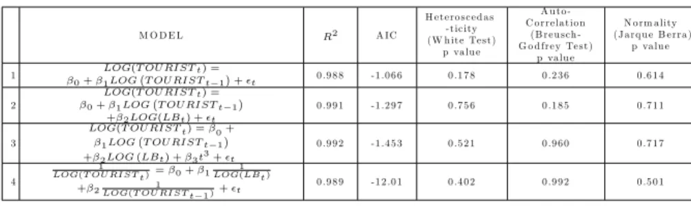
Table 5. Proposed Lagged Models by Ignoring Assumptions on Residuals
M O D E L R2 A IC H e t e ro s c e d a s -t ic ity ( W h ite Te s t) p va lu e A u to -C o rre la tio n ( B re u s ch -G o d fre y Te s t) p va lu e N o rm a lity ( J a rq u e B e rra ) p va lu e 1 LOG(T OU RISTt) = 0+ 1LOG T OU RISTt 1 + t 0 .9 8 8 -1 .0 6 6 0 .1 7 8 0 .2 3 6 0 .6 1 4 2 LOG(T OU RISTt) = 0+ 1LOG T OU RISTt 1 +2LOG(LBt) + t 0 .9 9 1 -1 .2 9 7 0 .7 5 6 0 .1 8 5 0 .7 1 1 3 LOG(T OU RISTt) = 0+ 1LOG T OU RISTt 1 +2LOG (LBt) + 3t3+t 0 .9 9 2 -1 .4 5 3 0 .5 2 1 0 .9 6 0 0 .7 1 7 4 1
LOG(T OU RIST t)= 0+ 1LOG(LBt)1
+ 2LOG(T OU RIST t 1)1 + t 0 .9 8 9 -1 2 .0 1 0 .4 0 2 0 .9 9 2 0 .5 0 1
In order to apply Least Squares Method for parameter estimation error terms should be uncorrelated, should have homoscedasticity and have a distribution with zero mean. On the other hand in order to make statistical conclusion about the sug-gested models, the error terms should be normally distributed or at least should be asymptotically normal. The normality assumption on the error terms is usually ig-nored in time series models because the size of data set is more than the regression model [1]. Therefore, as long as the error term is a white noise process, para-meter estimators are usually considered to be asymptotically normally distributed estimators.
It is shown that models in Table 3 and Table 4 cannot meet the assumptions. The reasons and solutions will be investigated. Overall conclusion about the existence
of problems that variables should be taken in the model hasn’t located in model or incorrect functional form has selected. Besides this explanatory variable(s) may have a functional e¤ect on the error terms directly [6]. In the …rst case, there isn’t any intervention because complete data which belong to other explanatory variables such as number of travel agencies, the countries share in advertising, tourism investments etc. On the period of covering analysis cannot be obtained. Problems arising from the second case will attempt to resolve by taking new vari-ables that involved lagged values of T OU RIST and LB. However models that have still unsolved problems will be eliminated at later stage. Models in Table 5 include the stationarity condition in addition to the assumptions. Because long term forecasts of non-stationary models have large standard errors, forecasts will be meaningless in terms of statistical inference. In the following section will also be taken to remedy this problem.
3. Handling The Problems Of Models
In application in order to solve the autocorrelation or heteroscedasticity problems of residuals, proposed transformations can eliminate these problems that exist at present or can also lead to occur new problems. In this study the problem of au-tocorrelation of residuals is solved with the Hildreth-Lu scanning procedure that is based on the generalized di¤erence method. The method is as follows; suitable generalized di¤erence transformation is done for model with the idea that residuals have the …rst order autocorrelation problems. The value of autocorrelation that makes the sum of squares minimum is used to transform the model by making suc-cessive adjustments in correlation according to the direction of correlation between residuals.
A point to be noted here is to …nd the appropriate value that can’t deteriorate other assumptions of the model. Sometimes other assumptions may be corrupted at SSE’s lowest value. Following steps will be taken to resolve the heteroscedasticity problem; explanatory variables or their functions that may cause heteroscedasticity problem will be determined by Breusch-Pegan-Godfrey Test and the problem will be considered whether it is resolved with White test by making suitable transforma-tions in the troubled model. For details of autocorrelation and heteroscedasticity problems and their methods of adjusting in Chapter 11 and 12 of [6].
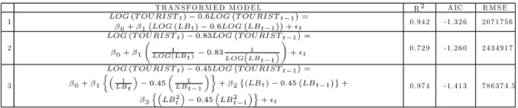
Autocorrelation problem of Model 1 and Model 3 in Table 3 has derived from residuals’ autoregressively related with the …rst degree. Therefore, transformed models have been proposed by taking …rst di¤erence. Model 2 in Table 3 has both autocorrelation and heteroscedaticity problems. Initially autocorrelation problem on residuals has been trying to resolve because its application is easier. Residuals of Model 2 have also autoregressive relationship with …rst degree, autocorrelation and heteroscedasticity have been eliminated by taking di¤erence one time with the transformed model. The transformed models for models in Table 3 are given below with their RMSE values.
Table 6. Transformed Models for Model in Table 3
T R A N S F O R M E D M O D E L R2 A IC R M S E
1 LOG (T OU RISTt) 0:6LOG T OU RISTt 1 =
0+ 1 LOG (LBt) 0:6LOG LBt 1 + t 0 .9 4 2 -1 .3 2 6 2 0 7 1 7 5 6
2
LOG (T OU RISTt) 0:83LOG T OU RISTt 1 =
0+ 1 LOG(LBt)1 0:83LOG LBt 11 !
+ t 0 .7 2 9 -1 .2 6 0 2 4 3 4 9 1 7
3
LOG (T OU RISTt) 0:45LOG T OU RISTt 1 = 0+ 1 LBt1 0:45 LBt 11 + 2 (LBt) 0:45 LBt 1 + 3 n LB2 t 0:45 LB2t 1 o +t 0 .9 7 4 -1 .4 1 3 7 8 6 3 7 4 .5
With analyzing Table 4 the models don’t have heteroscedasticity problems, whereas they have autocorrelation problem on their residuals. Autocorrelation problem will be solved by the Hildreth-Lu scanning process as in the previous models. The au-tocorrelation value that makes SSE minimum and eliminates auau-tocorrelation can’t create the heteroscedasticity problem as well, will be taken into account. The transformed model for Model 1 in Table 4 is same as Model 1 in Table 6. The transformed model for Model 3 in Table 4 rejects all variable associated with time trend. When these variables are removed from model the model is the same as Model 1 in Table 6. Thus Model 1 and Model 3 in Table 4 are eliminated from the proposed models. The …nal version of the proposed Model 2 in Table 4 is shown in the following table. Here to ensure the assumptions, coe¢ cient of t is excluded from this model.
Table 7. Transformed Models for Model in Table 4
T R A N S F O R M E D M O D E L R2 A IC R M S E
1
LOG (T OU RISTt) 0:2LOG T OU RISTt 1 = 0+ 1LOG (LBt) 0:2LOG LBt 1
+3t2+ t
0 .9 8 7 -1 .3 9 9 9 7 4 3 6 8 .1
Generally speaking for Table 5 the residuals of the four models provide the nec-essary assumptions. However the stationarity condition is necnec-essary for long-term forecast to be desirable. In addition the assumption of stationarity is important for statistical inference. Because of this the natural logarithm of T OU RIST has carried out unit root test. p value has found 0.8297 by applying ADF test in E-views Package Programme and has understood that the LOG(T OU RIST ) has unit root with …rst degree. p value has found 0.0000 by taking di¤erence one time for LOG(T OU RIST ) with the same test. Therefore the series contains one unit root. It’s revealed that LB has two unit roots by taking natural logarithm according to ADF test. LOG(LB) has been adjusted from unit root with ADF test. If LB is taken with unit root to regression model, this may cause spurious regression [5], [7]. Transformed model for Model 1 includes lagged model adjusted from unit root. The coe¢ cient of r2LOG(LB) is rejected in transformed model for Model 2 and when this variable is removed from the model, the model is same as trans-formed model for Model 1. Similarly time trend and r2LOG(LB) variables in
transformed model for Model 3 are rejected and when these variables are removed from the model, the model is same as transformed model for Model 1, too. The coe¢ cient of r2(1=LOG(LB)) variable is rejected in Model 4 and this variable is removed from the model. According to this transformed models for Model 1 and Model 4 are given in following table.
Table 8. Transformed Models for Model in Table 3
T R A N S F O R M E D M O D E L R2 A IC R M S E 1 r2LOG (T OU RIST t) = 0+ 1rLOG T OURISTt 1 + t 0 .5 9 8 -1 .0 9 5 1 3 0 1 6 4 4 2 r2 1 LOG (T OU RISTt) = 0+ 1r 1 LOG T OU RISTt 1 + t 0 .5 9 4 1 1 .8 8 1- 2 3 2 7 4 4 6 4. Forecasting
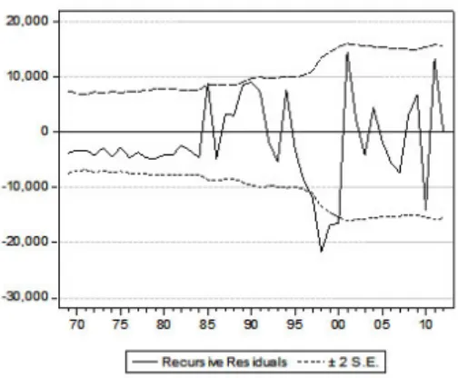
It is necessary that values of LB for forecast period (2013-2020) should be predicted or known to forecast with all transformed six models except for the models in Table 8. For this reason a model that will forecast the future values of LB is also needed. The primary aim of this section is to identify such a model. Various models have been tried for LB and the model which has the minimum RMSE value (ignoring other assumptions) is found as LBt= 0+ 1t + 2t2+ "tbecause residuals of this model have autoregressively related with second degree the problem has been tried to resolve with generalized di¤erence methods. Constant term and time trend variables have been removed because they are unnecessary. Additionally, considering the following recursive residuals chart the deviations are concentrated after 1985. The reason for this, it is possible to see that as the impact of intense terror events in the 1990s and Encouragement of Tourism Law enacted in 1982. With the aim of to purify this e¤ect, dummy variable has been put between the years of 1985-1995 then a second dummy variable has been put from 1996 to present day.
Both dummy variables have found individually signi…cant for either the constant term or the slope. The most suitable model has been obtained by adding second dummy variable as constant term with regarding to RMSE and model is as follows, LBt LBt 1+ 0:1LBt 2= 1DU M 2 + 2t2+ t (4.1) Making long-term forecasting is inconvenient because LB’s predicted model is non-stationary. Prediction equation for LB is as follows
LBt LBt 1+ 0:1LBt 2= 16132:83859 + 59:65046t2 (RM SE = 13903:47) (4.2) Holt’s Double Parameter Linear Exponential Smoothing Model is taken into con-siderations as an alternative forecasting model to the model above. Exponential
Figure 1. Recursive Residual Time Series Chart
Smoothing Method is used for r(LB) because two unit root and trend are in the model when unit root test is applied for LB with time trend. Smoothing equation, Lt= 0:722617r(LBt) + (1 0:722617)(Lt 1+ bt 1) (4.3) Trend equation, bt= 0:068487 (Lt Lt 1) + (1 0:068487)bt 1 (4.4) Forecasting equation, Ft= Lt+ bt; t 2012 (4.5) F2012+k= L2012+ kb2012; k = 1; :::; 8 (RM SE = 8670) (4.6) Since smoothing factor is close to one, forecasts are weighted related to actual values so the trend is less impact. Making 8 periods forecast of LB, two Parameter Linear Exponential Smoothing Model whose RMSE is smaller has chosen from two models above. However it should be reminded that short term forecast should be made because two proposed models for LB have a trend e¤ect.
With the aim to make comment about problems that may arise in the forecasting process estimates of coe¢ cients in the proposed transformed six models are given in the table below.
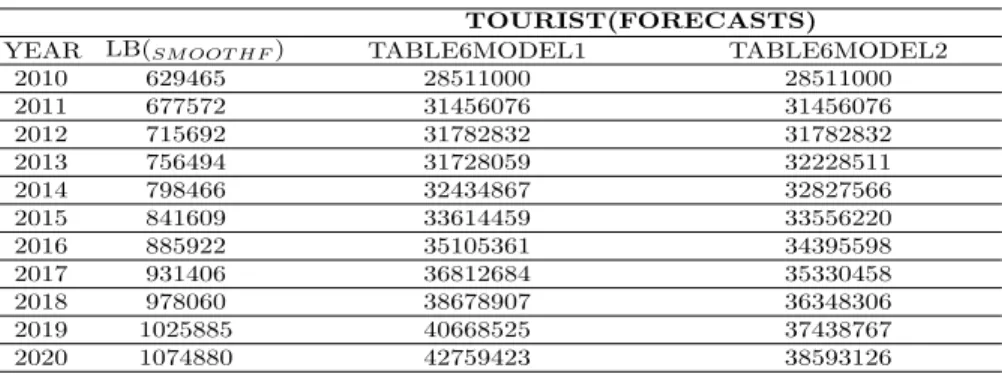
Although Model 1 and Model 2 in Table 6 comparison with other models have a higher value in terms of RMSE, more acceptable forecast has been obtained from these models. On the other hand Model 3 has minimum RMSE value but forecasts have increased until 2017, in later years have showed a decreased.
5. The Conclusions And Proposals
In generally as if forecast with these two models has an increase this situation is due to the increase of number of beds as 45000 each year in average. While making
Table 9. Estimations of Coe¢ cients for Transformed Models
Coe¢ cients Std. Dev. t-Stat. p value
TABLE6-MODEL1 0.846362 0.200167 4.228280 0.0001 1.112676 0.041663 26.70688 0.0000 TABLE6-MODEL2 4.992336 0.213971 23.33180 0.0000 -165.9087 15.26599 -10.86787 0.0000 TABLE6-MODEL3 7.955256 0.089705 88.68265 0.0000 -28563.15 5340.652 -5.348251 0.0000 6.56E-06 8.37E-07 7.834913 0.0000 -3.53E-12 1.02E-12 -3.461605 0.0012 TABLE7-MODEL1 4.259928 0.522739 8.149247 0.0000 0.809699 0.061085 13.25524 0.0000 0.000421 8.33E-05 5.051655 0.0000 TABLE8-MODEL1 0.106823 0.024755 4.315294 0.0001 -1.186619 0.148264 -8.003424 0.0000 TABLE8-MODEL2 -0.000458 0.000111 -4.106769 0.0002 -1.162159 0.146578 -7.928626 0.0000
forecasting modelling factors as developments of world economy, geographical and political situations of Turkey. Terror events in the country which e¤ect tourism activities directly negative of positive have been ignored.
In order to increase forecast accuracy related to the LB tourism areas which has been allocated to the tourism sector can be identi…ed with the approval of the Ministry of Tourism and Culture. Thus the number of beds’saturation point can
Table 10. Forecasts for Chosen Models
TOURIST(FORECASTS)
YEAR LB(SM OOT H F) TABLE6MODEL1 TABLE6MODEL2
2010 629465 28511000 28511000 2011 677572 31456076 31456076 2012 715692 31782832 31782832 2013 756494 31728059 32228511 2014 798466 32434867 32827566 2015 841609 33614459 33556220 2016 885922 35105361 34395598 2017 931406 36812684 35330458 2018 978060 38678907 36348306 2019 1025885 40668525 37438767 2020 1074880 42759423 38593126
be determined in the long-term. In this way the long-term forecasts of number of tourists by reducing the present momentum of LB can be made a little more sense with expost forecasting values.
References
[1] Akdi, Y. Zaman Serileri Analizi (Birim Kökler ve Kointegrasyon), 2nd Ed., Ankara, Gazi Kitabevi. 2010.
[2] Bahar,O ve Kozak, M. Türkiye Turizminin Akdeniz Ülkeleri ile Rekabet Gücü Aç¬s¬ndan Kar¸s¬la¸st¬r¬lmas¬, Anatolia: Turizm Ara¸st¬rmalar¬ Dergisi, Vol. 16, No 2, Güz, pp. 139-152, (2005).
[3] Chen, K.Y. Combining Linear and Nonlinear Model In Forecasting Tourism Demand, Expert Systems with Applications, 38, pp. 10368–10376, (2011).
[4] Dwyer, L. Gill, A. and Seetaram, N. Handbook of Research Methods in Tourism: Quantitative and Qualitative Approaches, Edward Elgar Pub, 2012.
[5] Granger, C.W.J. and Newbold, P. Spurious Regressions In Econometrics, Journal of Econo-metrics 2, pp. 111-120, (1974).
[6] Gujarati, M. and Porter, D. Temel Ekonometri, Translation from 5th Ed. (Ümit ¸Senesen and
Gülay Günlük ¸Senesen), ·Istanbul, Literatür Yay¬nc¬l¬k, 2012.
[7] Song, H. and Witt, S.F. Tourism Demand Modelling and Forecasting: Modern Econometric Approaches, Oxford: Pergamon, 2000.
[8] Song, H. and Li, G. Tourism Demand Modelling and Forecasting, A Review of Recent Re-search Tourism Management, 29 (2), pp. 203 – 220, ISSN 0261-5177, (2008).
[9] Song, H Tourism Demand Modelling and Forecasting: How Should Demand Be Measured?, Tourism Economics, 16 (1), pp. 63–81, (2010).
[10] Statistics of TUROFED are accessed from < http://www.turofed.org.tr/Bilgi-Edinme_13.aspx> on 27th June 2013.
Current address : Ankara University, Faculty of Sciences, Dept. of Statistics, Ankara, TURKEY E-mail address : [email protected], [email protected]