Integral action based Dirichlet boundary control of Burgers equation

Integral Action Based Dirichlbt Boundary Control

of

Burgers Equation

Mehmet Onder Efe Hitay Ozbay

Collaborative Center of Control Science Department of Electrical Engineering

The Ohio State University Columbus, OH 43210, U.S.A.

E-mail: onderefe@ieee.org

Dept. of Electrical & Electronics Eng. Bilkent Univ., Ankara TR-06533, Turkey

on leave from Dept. of Electrical Eng. The Ohio State University E-mail: ozbay@ee.eng.ohio-state.edu

Abstract-Modeling and boundary control for Burgers Equa- tion is studied in this paper. Modeling has been done via processing of numerical observations through singular value decomposition with Galerkin projection. This results in a set of spatial basis functions together with a set of Ordinar?. Differential Equations (ODEs) describing the temporal evolution. Since the dynamics described by Burgers equation is nonlinear, the corre- sponding reduced order dynamics turn out to be nonlinear. The presented analysis explains how boundary condition appears as a control input in the ODEs. The controller design is based on the linearization of the dynamic model. It has been demonstrated that an integral controller, whose gain is a function of the spatial variable, is sufficient to observe reasonably high tracking performance with a high degree of robustness.

I . IN’I‘RODUCTION

Modeling and control of infinite dimensional systems con- tain three major issues that need to be studied carefully. First issue is the modeling, i.e. collecting the representative data and exploiting several techniques to come up with a set of ODEs. The second issue is to separate the effect of extemal stimuli from the other terms by using the boundary conditions. The third issue is to design a controller that meets a set of prescribed performance criteria.

One should notice that the process under investigation is described over a physical domain (Z), the boundaries of which are the possible cntries of external stimuli. When the content of the obsen8ed data, say u(x, t j , is decomposed into spatial and temporal constituents (U(., t ) Y (@!(x),g(t))), the essence of spatial behavior appears as a vector of gains @(x)), which are functions of the spatial variable x E E, and the essence of temporal evolution appears as ODEs after utilizing the orthogonality properties of the spatial basis functions. Having this picture in front of us, the goal is to observe a predefined behavior at a set of physical locations by altering the boundary condition(s) appropriately.

Although we have roughly described the overall picture, when the problem is visualized for aerodynamic flows, a familiar difficulty is the presence of nonlinearity and strong couplings between the variables involved since the process is characterized by Navier-Stokes equations. Such a physical process reveals the entire richness of behavioral diversity through very strong nonlinear intemal interactions. A one-

dimensional “cartoon” of Navier-Stokes equations is the well- known Burgers equation studied extensively in the literature, When the modeling issue is taken into consideration, Proper Orthogonal Decomposition (POD) or Singular Value Decom- position (SVD) in cooperation with Galerkin projection are the popular approaches utilized several times in the literature,

[ 9 ] , [IO], [ I l l . The methods mentioned here use a library of solutions from the process, and separate the content of the data such that the spatial components (basis functions) reveal certain orthogonality properties and the temporal components synthesize the time evolution over those spatial basis functions. The decomposition yields meaningful information as long as the data contains coherent modes. One has to know that the result of POD or SVD schemes will be a set of basis functions accompanied by a set of autonomous ODEs.

Apparently the next issue, which is the separation of hound- ary condition(s) (or the control input(s)) from the remaining terms, plays a key role. For example Krstic describcs a neatly selected Lyapunov function in [SI, and the expression in its time derivative lets us apply integration by parts, then the boundary condition emerges in an explicit manner. Although the approach lets us manipulate DirichEt and Neumann type boundary conditions on Burgers equation, it is still tedious to follow the same procedure for Navier-Stokes equations. This is because of the high dimensionality and difficulty in finding an appropriate Lyapunov function. Therefore, utilizing the numerical techniques is a practical alternative to symbolic manipulation of variables. One major contribution of this paper is to explain how the issue of control separation is handled in numerical-data-based modeling approaches.

The third stage is the design of a suitable controller. In [I], a receding horizon optimal control approach is studied for Burgers equation with control input explicitly available in the Partial Differential Equation (PDE). The work presented by Bums et al [2], [3] demonstrates the stabilization by feedback

control. More explicitly, if ~ ( z , t ) is thc variable of interest, a control signal of the form y ( t ) =

-so

k(z)u(z,tjdz is sug- gested in [2], [ 3 ] to minimize a particularly defined quadratic cost function. It will later be discussed that the form of the control signal in this paper is y ( t ) = Ki(z,) Ji(ud(z,,p) ~ see e.g.

P I , PI,

131,

PI,

PI,

[61, VI, [SI.

u(z,>p))dp, which will be obtained upon linearization. The

aim is the tracking based on the information obtained from a given measurement point x,. The way we set the gain

Ki(z,)

is based on the gain margin analysis. An alternative approach to the design of an optimal controller for Burgers equation is presented in [4]. This reference demonstrates the Cole-Hopf transformation to obtain a linear diffusion type problem. The drawback of this approach is twofold: First it converts the cost function into an equivalent but a complicated one, second, the applicability of the technique is highly dependent on the structure of the goveming PDE. For this reason, approaches such as the one in [ 5 ] are developed to extract valuable information from numerical data. A quadratic cost function is defined and the process of minimization is achieved through conjugate gradient method. KrstiC [7] presents a backstepping control by assuming actuators at the boundaries. In [6], the viscosity coefficient is assumed to be unknown, and an adap- tive control scheme has been presented with particularly for Burgers equation.

This paper is organized as follows: The second section presents briefly the SVD technique and its relevance to the modeling strategy. In the third section, development of the reduced .order model for the Burgers equation is analyzed. Section 4 describes the control problem. The fifth section presents the simulation results and the concluding remarks are given at the end of the paper.

11. SINGULAR VALUE DECOMPOSITION

Consider d(tti) = (2L(o,t,),2L(Azlth), . . . , u((lY- l)Az,th)), which constitutes a snapshot containing the data (U(., t h ) ) observed from a process at time t = t h . If the data is recorded over a grid having

S

time points and N spatial locations, the ensemble, D, will be a matrix of dimensions

S

x

N; and

dth)

-

will be a row of D (or a snapshot from the process) for the observation at time t = t i . Singular value decomposition separates the content of

D

as follows:

D

= CIA@, (1)

where denotes the transpose. In (I), U is an

Sx

S orthogonal matrix, A is an S x N matrix containing the singular values

in

the diagonal with rest of the entries being equal to zero, and V is an N x N orthogonal matrix. The rows of A contain the singular values in decreasing order, i.e. U I

2

uz

2

. .

.

2

U N .

Defining fl:=UA lets us rewrite ( I ) as follows

where and g k correspond to the kth columns of the matrices Cl and V respectively. The representation in (2) contains the full set of modes existing in the ensemble D , if however the expansion is performed utilizing M modes, where

M

<

N, one can obtain an approximate reconstruction of the information content of D ; and (2) can be rewritten as D Y C E 1 g k g i . The accuracy of this representation

is given by the percent energy captured. This measure is described as

E

= 100(Ck=,

rk)/(Cf=,

ub) The most useful aspect of the representation in (2) is the fact that it contains the temporal information in

0

and spatial information in V matrices. Therefore, one can set desired energy percentage

( E ) , determine the required number of modes ( M ) and identify the corresponding columns of

fl

and V to obtain a reduced order model given below:

M

M

u(z,t) a k ( t ) @ k ( z ) , (3)

P = l

where O k ( t ) is a function oftime, whose value at timet =

iAt

is is equal to the value seen in the ith entry of g k , where i = 1,2,. . . ,S. Similarly, G k ( z ) is a function of x, and it synthesizes the entries seen in 2: at every spatial grid point, say

x

=

jAz,

where j = 1 , 2 , . . . , N . Therefore, one can visualize the relation between the observed data and these new variablesas

(D)ij

Y

E,"=,

cuk(iAt)@&'Az). This representation is useful for modeling purposes due to the orthonormality of the columns of the matrix V.

Note that, a major issue in the field of reduced order mod- eling of infinite dimensional systems is to examine the nature of error introduced by equating the both sides of (3). Although in terms of preserving the energy, one may approximate the original dynamics fairy well, the nature of lost information is still an open question. In what follows, obtaining the reduced order models based on the approximation in (3) is discussed by assuming the equality.

111. REDUCED ORDER MODELING OF BURGERS SYSTEM

In this section, we apply the SVD technique to the viscous Burgers equation described by

where E = 1 is a known process parameter, z E 2 and

Z = [0,1]. The problem is specified with the initial condition

u(z, 0) = 0 Vx, the homogeneous boundary condition at z = 0 as u(0, t ) = 0 and Dirichlet boundaly condition at z = 1 as

u(1, t ) = y(t), where y ( t ) is the extemal input of the system. Since the SVD scheme yields the decomposition

inserting this into (4) results in

Since VT=V-', (G1(z),G3(z)) =

So,

where ~ 5 % ~ is the well-known Kronecker delta function. Taking the inner product

where

*

denotes the elementwise product operator.

Since the extemal inputs are not seen explicitly in (S), in what follows, the terms will be manipulated such that the two

dynamics, namely the one enters directly with the boundary condition and the one inherent in the spatial behavior caused by the boundary condition are separated properly. The driving point is to notice that the soluion in (5) must be satisfied at the boundaries as well. This gives the following information;

h1

U ( 1 , t ) =y(t) = C(Yi(t)@i(l). (9)

% = I

Or a l ; ( t ) @ k ( ~ ) = y(t) -

cffl(l

- & k ) c ~ i ( t ) * ~ ( l ) . Inserting this into the second summation in (8) yields

in the linearizcd system's state space representation, (18), and the controller gain is likely t o be a function ofthe measurement T

-

B ( a )

=

(

nTBia

( ~ ' B z g . . . ~ u ~ B 8 . r ~

)

: _{(15) point,}

%,,,,

where ( B k ) i j =

@i(zo)(@i(zo)

*&(z")).

Rewrite (19) as

(20)

N ( z m ,

3) (C)k = & ( l ) > (16) H ( s ) = -, V ( s ) and (D)ki = D i ( 1 ) W ) . (17)

IV. CONTROL PROBLEM

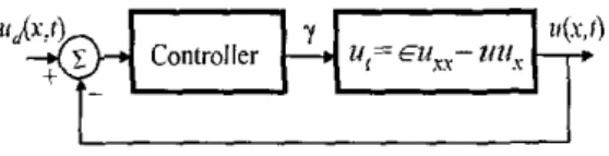
Consider the feedback loop illustrated in Figure I . The dynamic model in (13) provides the tcmpurdl variables. Since the point of measurement,

z

=

z

,

,

is known, the output equation in (5) lets us calculate the solution of the PDE in

(4). Therefore the observation is a point observation, and the

desired signal ( u d ( z , t ) ) is imposed for that particular location. Clearly the goal is to observe the desired behavior ud(z,, t ) at an arbitrary 5 , t: (0,l).

I

I

Fig. I. Block diagram ofthe control system

If (13) is linearized around a = 13, one gets the linear dynamic model given by

-

iu = A g

+

c y , (18)

where A and _C are as defined in (14) and (16) respectively. With these quantities, one can calculate the transfer function

where s is the Laplace transform variable and

r(s)

:= L { y ( t ) } and

z,

t (0,l).

The modeling studies results in a A matrix such that the eigenvalues of A have negative real parts. Therefore, a change in the point of measurement will affect the locations of the zeros of the transfer function above (due to the output vector - @(zm)), and the stability properties will be preserved for Although one can suggest many different kinds of control strategies for the linearized system, the simplest one i s the integral control. Another encouraging factor is that it makes the open loop transfer function Type-I and constant values are tracked with zero steady state error.

Once the control action is confined to pure integral action, the forthcoming issue is to set its gain X i . Intuitively, one

might guess that once the Dirichet boundary control is applied from the I-boundary, the distribution of it over 5 is realized by the basis functions (@(z)), which appear as the output vector

vzm

t (0; 1).

The open loop transfer function without the gain parameter becomes

In Figure 2 , the gain margin for the transfer function in (21) is drawn by a dashed line for

z

,

E (0,l). The solid line in Figure 2 depicts the chosen controller gain, K,(z,) given by

which is less than the critical gain for z, t (0.0375;l). Apparently, the control at the I-boundary has no effect on 0-boundary since u(0, t ) is specified independently. The calcu- lated gain margin and the chosen one intersects in the relatively broad vicinity of 0-boundary, below this critical value, the closed loop system is unstable with the above selection of Ki (2,). D.yIPdcmiia,"al".~~lld C"0r.n Gain

1

I\.

... . . . . . . ... . . . . I v 0 0 , 0 2 0 1 0 4 0 5 D I 0, O B 0 s

,

1 00

R g 2 Gain margin (Dashed line) and the chosen controller gain (Solid line)

In the next section, the details concerning the simulations are presented in detail.

v.

SIMULATIONS A N D DISCUSSION A. Modeling Results

For obtaining a set of ODES characterizing the dominant dynamics, the PDE in (4) has been solved by using Crank- Nicholson method (See [121) for a set o f boundary conditions according to the procedure discussed. The solution has been obtained over a grid with N = 100 (Az = 1/99) spatial locations, and the time interval (At) has been chosen as lmsec

(S = 1001). As the test inputs, we have considered constant, increasing, decreasing and periodic functions while applying these from I-boundary and holding the 0-boundary at zero. Since these are the likely cases in the time behavior of an external stimulus, the result is expected to capture all of them to some extent. Having obtained the solutions, SVD procedure is applied for each case. We have observed that keeping five modes (A4 = 5) captured in average 99.84% o f the total energy described in the second section.

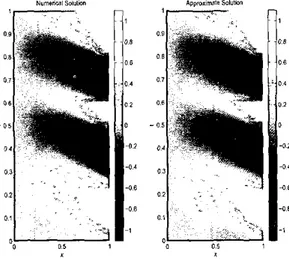
The obtained basis functions have been approximated by Sth order polynomials of z. The coefficients of these polynomials are found by utilizing least mean squares approach. In all test cases. we observed a very good similarity between the basis functions, and to generalize the basis set, we used the averagc o f them. Use o f these polynomials in (14) through (17) has let us obtain the system matrices and uncertainty terms. 1r1 Figure 3, modeling results for an exemplar case are illustrated. The arbitrarily chosen boundary conditions are y(t) =

{

sga(sin(5st)), 0.5s 5 t 5 Is.

As seen from Figure 3, the numerical solution illustrated on the left subplot is reasonably similar to the approximate solution obtained through the reduced order modeling scheme discussed in the second section.

sin(4?rt), 0

5

t

5

0.5s

N u " , SOlYlm

: . i J4

,

. 1

Fig. 3. A comparison of the numerical solution and appmnimate solution

B. Cuntrul Sludies

In order to demonstrate the control performance of the proposed control scheme, we study two different regimes in the course of a single control trial. According to this

0.75, 0 5 t

5

30s 0.25, t

>

30s. '

As the reference signal, we choose a repeating train of pulses given as

The obtained results have been depicted in Figure 4. The upper left subplot shows both the reference signal and the observed output together. The upper right subplot illustrates the difference between them. Apparently the way the output approaches positive value displays an overdamped behavior while there are damped oscillations around the negative de- sired value. This is clearly due to the nonlinearity ofthe system dynamics. Qualitatively, the speed o f the response is not fast enough but the tracking capability is admissible.

Fig. 4. Simulation resulls for an exemplar control trial

The bottom left subplot of Figure 4 demonstrates the evolu- tion of the boundary control. Referring to (23) with u(0, t ) = 0 boundary condition, the result stipulates that the same refer- ence signal can be tracked with small-magnitude boundary excitations. As the measurement point moves towards the 0- boundary, the same tracking task will require comparably high magnitude boundary excitations.

The lower right subplot of Figure 4 illustrates the gain o f the controller. The values of K,(z,) can approximately be justified also from Figure 2.

It should also be noted that, due to the space limit, the presented test case is only one of the many such cases contain- ing different forms of mentioned difficulties, and the results are all very successful. The ultimate goal of this research is to demonstrate that an appropriate feedback control strategy can be devised for aerodynamic flows displaying turbulent behavior.

which clearly suggests that the point of measurement (z,) undergocs a radical change at time t = 30sec. Therefore, alleviating the difficulty caused by such a large change when considered with the structural simplicity constitutes a design challenge.

VI. CONCI.USIONS

This paper discusses the modeling and control of Nonlinear Infinite Dimensional Systems (NIDS). The approach is based on the numerical observations, therefore it is applicable not only to Burgers equation but also to a class of NIDS, whose

solutions are, dominated by coherent modes, The modeling approach and the way how it constitutes an integral part of a feedback control strategy is discussed. SVD technique is used in the modeling stage, then the temporal and spatial information have appropriately been separated into ODES and spatial gains respectively. It has been observed that a spatially- variable-gain integral controller controls the linearized system reasonably well. Since the output equation given by (5) introduces spatially-variable terms, gain margin becomes a function of

x.

The chosen form of the controller gain is inside the admissible region, and results justify the theoretical claims. The structural simplicity of the controller is another prominent feature that should he highlighted.

The major contribution of this paper is to clarify how control terms are separated if the numerical techniques, such as SVD or POD are utilized.

ACKNOWLEDGMENTS

This material is based on research sponsored by Air Force Research Laboratory, Agreement no: F33615-01-2-3154,

The authors would like to thank Prof. M. Samimy, Dr. J.H. Myaa, Dr. J. DeBonis, Dr. M. Debiasi, X. Yuan and E. Carahallo for fruitful discussions in devising the presented work.

REFERENCES

[ I ] M. Hinze and S. Volkwein, "Analysis of Instantaneous Control for Burgers Equation," Nonlinear Anolysis, 50, pp. 1-26, 2002.

[2] J.A. Bums, B.B. King and L. Zietsman, "On lhe Computation of Sin- gular Functional Gains for Linear Quadratic Optimal Boundary Control Problems," Proc. of the 3'd Theoretical Fluid Mechanics Meeting, June 24-26, Si. Louis, AlAA 2002-3074, 2002.

[3] J.A. Bums, B.B. King. A.D. Rubio a n d L . Zietsman, "Functional Gain Compuiatians for Feedback Control of a Thermal Fluid," Roc. of the

Y d Theoretical Fluid Mechanics Meetin& June 24-26, St. Louis, AlAA 2002-2992, 2002.

[4] R. Vedantham, "Optimal Control of the Viscous Burgers Equation Using an Equivalent Index Method," J of Global Optimization, 18, 255-263,

151 H.M. Park and Y.D. Jang, "Control of Burgers Equation by Means of Mode Reduction." h i . J. ofEng. Science, 38, pp. 785-805, 2002.

[6] W.-J. Liu and M. KrstiC. "Adaptive Control of Burgers' Equation With Unknown Viscosity," Inl. J Adaptive Contml ond Signal Pmessing 15. 8~1745.766. 2001.

[7] W.-J. Liu and M. Krstit, "Backstepping Boundary Control of Burgers' Equation With Actuator Dynamics," Systems and Contml Letters, 41, [SI M. KrstiC, "On Global Stabilization of Burgers' Equation by Boundaly

Control:' Systems ond Contml Letlers, 37, pp.123-141, 1999. 19) S.S. Ravindran, "A Reduced Order Approach for Optimal Control of

Fluids Using Proper Orthogonal Decomposition," In!. J /or Numerlcol Methods in Fluids, v.34. pp.425-488, 2000.

[ I O ] H.V. Ly and H.T. Tran, "Modeling and Control of Physical Processes Using Proper Orthogonal Decomposition," Mathematical and Computer Modelling of Dynamical Systems, v.33, pp.223-236, 2001

[ I l l S.N. Singh. J.H. Myatt, G.A. Addington, S. Banda and J.K. Hall, "Op- timal Feedback Control of Vortex Shedding Using Proper Orthogonal Decomposition Models,'' Trans. of the ASME: J of Fluids Ens, v.123, pp. 618, September 2001.

[I21 S.J. Farlow, Partial Differential Equations for Scientists nnd Engineers,

Dover Publications Inc., New York. pp. 317-322, 1893.

1 2000

pp.291-303. 2000.