Material characterization by using high velocity modes

Ί

■VS?·

/ д э и

MATERIAL CHARACTERIZATION BY USING HIGH

VELOCITY MODES

A THESIS

SUBMITTED TO THE DEPARTMENT OF ELECTRICAL AND ELECTRONICS ENGINEERING

AND THE INSTITUTE OF ENGINEERING AND SCIENCES OF BILKENT UNIVERSITY

IN PARTIAL FULFILLMENT OF THE REQUIREMENTS FOR THE DEGREE OF

MASTER OF SCIENCE

By

Goksen Goksenin Yaralioglu

August 1994

ТРѴ

4 \ Ψ .2 .^

-У з^ Ί 3 3 4

I certify that I have read this thesis and that in my opinion it is fully adequate, in scope and in quality, as a thesis for the degree of Master of Science.

Prof. Dn Hayrettin K<wmen(Supervisor)

I certify that I have read this thesis and that in my opinion it is fully adequate, in scope and in quality, as a thesis for the degree of Master of Science.

Prof. Dr./Abdullah Atalar (Co-supervisor)

I certify that I have read this thesis and that in my opinion it is fully adequate, in scope and in quality, as a thesis for the degree of Master of Science.

Assoc. Prof. Dr. Ayhan Altıntaş

I certify that I have read this thesis and that in my opinion it is fully adequate, in scope and in quality, as a thesis for the degree of Master of Science.

(Q o k d —

Assist. Prof. Dr. Orhan Ankan

Approved for the Institute of Engineering and Sciences:

Prof. Dr. MehgjecBaray

ABSTRACT

MATERIAL CHARACTERIZATION BY USING HIGH

VELOCITY MODES

Göksen Göksenin Yaralıoğlu

M.S. in Electrical and Electronics Engineering

Supervisor: Prof. Dr. Hayrettin Köymen

Co-supervisor: Prof. Dr. Abdullah Atalar

August 1994

Acoustic microscopy is one of the most powerful tools for non-destructive material characterization. Excited modes on the materials are responsible for the high contrast obtained in the images. However, conventional lenses suffer from multi-mode excitation. Lamb wave lens proposed earlier overcomes this difBculty. It insonifies material surface at only one incidence angle.

In this thesis, material characterization ability of high velocity modes for loaded single layered materials by using Lamb wave lens is investigated. The validity of the theory is checked by comparing simulated and measured V(z) curves obtained from specially prepared sample.

Keywords : Acoustic microscopy, non-destructive material characteriza­ tion, Lamb wave lens, high velocity modes, V{z) curves.

ÖZET

YÜKSEK HIZLI DALGALARI KULLANARAK MALZEME

TANIMLAMASI

Göksen Göksenin Yaralıoğlu

Elektrik ve Elektronik Mühendisliği Bölümü Yüksek Lisans

Tez yöneticileri: Dr. Hayrettin Köymen

ve Dr. Abdullah Atalar

Ağustos 1994

Akustik mikroskop zarar vermeden malzeme tanımlamalarında kul­ lanılan en güçlü gereçlerden biridir. Malzeme yüzeyinde uyarılan modlar, görüntülerdeki yüksek zıtlığı sağlar. Ancak, alışılmış merceklerin birden çok mod uyarma problemi vardir. Daha önce önerilmiş Lamb dalgası merceği ile bu güçlüğün önüne geçilebilir. Bu mercek, malzeme yüzeyini sadece bir geliş açısında aydınlatır.

Bu tezde, yüksek hızlı modların Lamb dalgası merceği kullanılarak, yüklenmiş tek katmanlı malzeme tanımlama yetenekleri araştırılmıştır. Ku­ ramın geçerliliği, özel olarak hcizırlanmış bir örnekten alınan deneysel ve ben­ zetim V(z) eğrilerinin karşılaştırılmasıyla kontrol edilmiştir.

Anahtar Kelimeler : Akustik mikroskop, zarar vermeden malzeme tanımlaması, Lamb dalgası merceği, yüksek hızlı modlar, V{z) eğrileri.

ACKNOWLEDGMENTS

I would like to thank to Dr. Hayrettin Köymen for his supervision, guid­ ance, suggestions and encouragement through the development of this thesis.

I would also like to thank to Dr. Abdullah Atalar for invaluable suggestions and Dr. Ayhan Altıntaş and Dr. Orhan Arikan for reading and commenting on the thesis.

It is a pleasure to express my thanks to all my friends. Aydın, Feza, Çağdaş, Kenan, Gökhan, Ayhan, Fatih, Engin, İbrahim, Serdar, Ece, Hakan, Gürkan, İlkay, Berna, Bihter, Yeşim, Kırdar, Erhan and my sister Devrim for their lovely patience.

TABLE OF C O N T E N T S

1 INTRODUCTION 1

2 THEORY 3

2.1 Reflection and Refraction at the Solid/Solid B o u n d a r y ... 3

2.2 Reflection and Refraction at the Fluid/Solid B o u n d a ry ... 6

2.3 Surface W aves... 7

2.4 Leaky Waves ... 9

2.5 Generalized Lamb W aves... 9

2.6 Sezawa W aves... 13

2.7 Complex Analysis of Reflectance F u n c tio n ... 15

2.8 Lamb Wave L e n s ... 21

2.9 Lens D e s ig n ... 24

2.10 Lateral W aves... 25

3 SIMULATION 26 3.1 Calculation of the Reflection Coefficient for the multi-layered solids... 26

3.2 Effect of Losses in S o lid s... 28

3.4 Calculation oi V { z ) ... 33 4 V{z) R ESU LTS F R O M H IG H V E L O C IT Y M O D E S 37 4.1 Experimentation ... 37 4.2 V{z) R esults... 39 5 C O N C L U S IO N 44 A D E R IV A T IO N O F R E F L E C T IO N AN D R E F R A C T IO N C O ­ E F F IC IE N T S 46

A.l Reflection and Refraction for Horizontally Polarized Shear Wave Incidence... 46 A.2 Reflection and Refraction for Vertically Polarized Longitudinal

Wave In cid en ce... 47

B H A N K E L T R A N S F O R M P A R A M E T E R S 49

C IS O T R O P IC A C O U S T IC P A R A M E T E R S 51

LIST OF F IG U R E S

2.1 Longitudinal incidence to solid/solid b o u n d ary ... 3 2.2 Normal incidence to the boundary... 5 2.3 Reflection Coefficient (w ater/alu m in u m )... 7 2.4 Reflected field due to the bounded beam incident at leaky wave

a n g le ... 10 2.5 Reflection Coefficient (water/al(30/i)/silicon(substrate)) at 110

MHz... 11 2.6 Loaded Case. Dispersion Curves and Schoch Displacement of 30

micro-meter thick aluminum layer on silicon substrate... 12 2.7 Stiffened Case. Dispersion Curves, Schoch Displacement and

Reflection Coefficient (at 75 MHz.) of 30 micro-meter thick chromium layer on copper substrate... 14 2.8 Pole-zero, magnitude and phase plot of 'R .{ k x ) ... 15 2.9 Pole-zero, magnitude and phase plot of ^ { k x ) ... 16 2.10 Pole-zero plot and reflection coefficient of 400 micro-meter thick

copper layer on steel substrate at 5 MHz... 16 2.11 Dispersion curves for 30 micro-meter thick aluminum layer on

silicon substrate. (Poles of reflectance f u n c tio n ) ... 17 2.12 Trajectories of poles and zeros of LR, M2 and M3 modes . . . . 18 2.13 Trajectories of poles and zeros of M4 and M5 m odes... 18

2.14 Trajectory of poles and zeros of M6 mode ... 19 2.15 Trajectory of poles and zeros below longitudinal critical angle . 20 2.16 Trajectory of poles and zeros of LR mode in stiffened case . . . 20 2.17 Lamb Wave L e n s ... 21 2.18 Reflection Coefficient (water/copper(400/i)/steel(substrate)) at

5 MHz... 22 2.19 Simulated V{z) curve from 400 micro-meter thick copper layer

on steel substrate. Lens angle=37.63°,Incidence angle=29.38°, upper radius=5.0 mm, lower radius=9.0 mm, frequency=5 MHz. 22 2.20 Simulated V(z) curve from 400 micro-meter thick copper layer

on steel substrate. Lens angle=31.00°,Incidence angle=24.05°, upper radius=5.0 mm, lower radius=9.0 mm, frequency=5 MHz. 23

3.1 Geometry of a multi-layered s o l i d ... 27 3.2 Reflection Coefficient (water/epoxy(60/i)/aluminum(substrate))

at 5.0 MHz. Solid line indicates the case with no longitudinal nor shear attenuation... 30 3.3 Reflection Coefficient (water/epoxy(60/i)/aluminum(substrate))

at 5.0 MHz. Longitudinal attenuation is fixed at 1351.0 neper/m eter...30 3.4 Pole-zero plot of the reflectance function (60 micro-meter epoxy

layer on aluminum substrate) at 5.0 MHz. for different longitu­

dinal and shear attenuation coefficients... 31 3.5 Pole-zero plot of the reflectance function (60 micro-meter epoxy

layer on aluminum substrate) at 5.0 MHz. for longitudinal at­ tenuation = 5.407 X 10“ ** and shear attenuation = 6.0 x 10“ ** 31

3.6 Scalar potentials on the lens geometry ... 33 3.7 Magnitude of potentials at plane-1 and plane-2... 36 3.8 Angular distribution at the lens aperture... 36

4.1 Electronic s e tu p ... 38 4.2 Calculated and experimental V{z) from 500 micro-meter copper

on steel substrate. Operation frequency is 6.65 MHz. Upper radius=3.91 mm Lower radius=5.95 m m ... 39 4.3 Reflection CoeflBcient of 500 micro-meter thick copper layer on

steel substrate for good bond and dis-bond cases at 32 MHz. . . 40 4.4 Calculated V (z) from 500 micro-meter copper on steel substrate

for good bond and dis-bond cases at 32 MHz... 41 4.5 Calculated and experimental V{z) from 500 micro-meter copper

on steel substrate. Operation frequency is 32 MHz... 42 4.6 Dispersion curves and Schoch displacement of 500 micro-meter

thick copper on steel substrate for good bond...43

A.l Horizontally polarized shear incidence to solid/solid boundary . 46 A.2 Vertically polarized longitudinal incidence to solid/solid boundary 48

Chapter 1

INTRODUCTION

Acoustic microscopy finds a wide range of applications [1], [2], [3]. Material scientists measure elastic parameters of the materials, velocity and the atten­ uation of surface acoustic waves in materials and anisotropy [4]. It can be also used to measure the thickness of the layered materials [5] and to investigate adhesion properties of bonds [6]. Biologists use this apparatus to obtain elastic properties of cells in vivo and in vitro.

In industry, by using cicoustic microscope, it is possible to detect cracks in materials, flaws in coatings and delaminations in integrated circuits.

As in the case of optical microscope, acoustic microscopes use the fact that waves change velocity while crossing an interface between two different materials. Acoustic velocities may differ up to ten times from one material to another. In the case of plane wave incidence, acoustic lenses refract the wave into spherical equi-phase surfaces. On the other hand, the change in velocity of the light is small, hence refracted waves can not be shaped into spherical waves.

Acoustic lenses are made from aluminum or sapphire. They couple lon­ gitudinal waves, generated by the transducers, to a liquid, usually water, in which the sample under investigation is placed. Reflected waves from sample are again collected by the lens and by recording the returned echo while the lens is scanned in the X — Y direction, image of the sample is taken. One can also obtain V{z) or V (/) curves, by changing the distance between specimen and the lens, or the frequency while keeping the distance fixed. V(z) and V {f) curves are very useful for material characterization.

Conventional lenses of spherical geometry are commonly produced. These lenses insonify specimen surface at a continuum of incidence angles. Hence, all possible modes are excited at the same time. V{z) curves obtained in this fashion are difficult to interpret, since they contain contributions from all excited modes and sub-surface images from layered materials are cluttered by simultaneously excited modes.

The Lamb wave lens, proposed earlier [7], overcomes the multi-mode exci­ tation problem. In Lamb wave lens, spherical cavity of the conventional lens is replaced by a conical recess. Layered materials are insonified at fixed angle by conical waves. Hence, only one of the possible modes are excited if the incidence angle matches with the mode critical angle. The Lamb wave lens has higher sensitivity to excited mode, since it does not waste power on ex­ citing other modes. However, its surface imaging properties are not as good compared with the spherical lens, due to the its poor focusing property.

In this study, characterization ability of high velocity modes for one layered, loaded materials is investigated by using Lamb wave lens. The velocity of these modes are higher than both the layer and the substrate’s shear velocity. They are excited for incidences below cut-off angle. Dispersion curves for these modes are also given.

In Chapter 2, acoustic boundary problems are revisited in the cases of both solid/solid and liquid/solid interfaces. Lamb wave modes which exists on the layered materials are described. Complex analysis of the reflectance function is considered with emphasis on how poles and zeros move on the complex plane with frequency. The theory of V{z) curves obtained by using the Lamb wave lens is given. In Chapter 3, the calculation of the reflection coefficient and the dispersion curves which shows the phase transitions of the reflection coefficient are explained. The simulation program that gives the V(z) curves are described. The experimentation setup is also presented in this chapter. Chapter 4 deals with the experiments and results. Finally, conclusions and discussions, chapter 5, concludes this work.

Chapter 2

THEORY

2.1

R eflection and R efraction at th e S o lid /S o lid

B oundary

Acoustic boundary condition problems are more complicated than electromag­ netic boundary problems since there exist two types of acoustic waves. It is necessary to consider contributions from both longitudinal and shear waves and polarization in the medium, to satisfy boundary conditions.

An acoustic interaction at a boundary is shown in Figure 2.1. To satisfy boundary conditions at any point on the interface, incoming, reflected and refracted waves must have the same phase variation at z=0 plane [8].

This implies that:

kx = kii sin(^/i) = ki2 sin(^/3) = k^i sin(^,i) = k^2 sin(^,2), (2.1)

and,

^11 — ^12 j (2.2)

where kn, ki2, A;,2 are the longitudinal and the shear wave propagation constants in the medium.

Equation 2.1 is Snell’s law which can also be expressed as follow:

vii Vl2 Vai Vs2

sin(0/l) sin(0/3) sin(0,i) sin(^,2) ’ (2.3) Longitudinal and the shear wave velocities in the medium are denoted by

f^i2·, ^sit ^s2· Propagation direction is found from Snell’s law.

The amplitudes of the reflected and the transmitted waves can be calculated by using the following boundary conditions:

1. The normal component of the longitudinal stress (Trz), 2. The tangential component of the shear stress (Tyz + Txz),

3. Both the normal (uzz) and the tangential {uxx + Uyy) components of the displacement,

must be continuous [9].

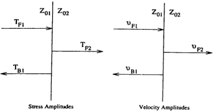
In the case of normal incidence, reflected and transmitted waves have the same type with the incident wave and stress reflection and transmission coef­ ficients are given by the following formulae:

Tf2 Tfi Tbi _ j, Zq2 — Zo\ Tfi Zq2 + Zq\ (2.4) 2^02 = T r = l - f r T = - ^ - ° V - · ■^02 + ■^01 (2.5)

^01 -02 *F1 ^01 V_{F l} -02 F2 V>_F2 B1 B1

Stress Amplitudes Velocity Amplitudes

Figure 2.2: Normal incidence to the boundary

^01,02 are the acoustic impedances (shear or longitudinal) of the media. For

a plane wave propagating in the forward direction, it is given by:

Z

-^0 —---,

Vf (2.6)

where Tp and vp denote stress and velocity amplitudes in the forward direc­ tion, respectively. For the backward direction, Zq relates stress and velocity

amplitudes as follows:

Zo =

V B

(2.7)

Using equations 2.6 and 2.7 one can drive the formulae for velocity reflec­ tion and transmission coefficients:

vbi Vpi n = - Ft = Zni — Zl02 Zo2 + ■2ni (2.8) _ rji nP— 1 r< 2^02 — Tu — Tt — 1 Fv — V p i ¿/Q2 T ^0 1 (2.9)

The simplest case of the oblique incidences is the horizontally polarized shear wave incidence in which the shear displacement lies in the xy plane and hence is parallel to the boundary. Reflected and transmitted waves are only shear waves. Stress reflection and transmission coefficients aire given by [8]:

Tr =

Tt = 2^1 cos(0,i)

Zai cos(0,i) - Z,2 COs(^,2) ’ (2.11)

where and Z,2 are the shear impedances of the upper and the lower half spaces, respectively. Refraction angle, 0,2, is calculated from Snell’s law.

0,2 = arcsin ( sin(0,i)— ^

V

w,i/

In Appendix A the derivation of the formulae in the case of horizontally polarized shear wave and vertically polarized longitudinal wave incidences are given, respectively.

2.2

R eflection and R efraction at the F lu id /S o lid

B ou n d ary

To solve fluid/solid boundary problems, boundary conditions given in previous section must be modified. Since fluid can slide freely in the tangential direction, horizontal displacement is no longer continuous. Liquid media can not support shear waves so shear stress in liquid is zero. Due to the continuity of shear tangential stress, it is set to zero on solid surface as well.

It is more convenient to use pressure amplitude instead of stress in liq­ uid. Reflection coefficient, which relates the incident pressure amplitude to the reflected amplitude, in terms of tangential propagation vector is given by [11]:

n { h ) =

where kq,ki,K3 are the propagation constants in liquid and solid, respectively. Densities are denoted by po and pi. If dependence is assumed and positive z-axis is taken as shown in figure 2.1, then:

Ki

j yjk^ — k^ otherwise (2.14)

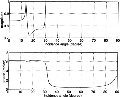
When 0 < kx < ki, reflection coefficient is real and there is no phase variation. If k^ is equal to ki, ^{kx) = 1 and all incident power is reflected. Between ki and ¿0, phase of the 'R.{kx) changes with incidence angle.

Tangential wave number, kx, is a complex number. I t’s real part is given by kosin{$i), where Oj is the incidence angle and ko is the wave number in liquid. Complex part represents an exponential decay in amplitude. K{kx) has branch points at =¡=¿0, T K , complex poles at kp and zeros at the

complex conjugate of the poles. One of the pole-zero pairs is close enough to real axis {kp == ^ + j o R where a n / 0 « 1) so that it is observed as sharp phase transition in the reflection coefficient (Figure 2.3).

Figure 2.3: Reflection Coefficient (water/aluminum)

2.3

Surface W aves

Besides longitudincd and shear waves, there exists the third kind of wave which is called Surface Acoustic Wave [9]. The idea of surface waves is first introduced by Lord Rayleigh [10]. They are mixture of longitudinal and shear waves traveling along the surface of a semi-infinite medium with a common phase velocity. The wave energy is mainly concentrated at the surface and falls off

rapidly to the interior.

Rayleigh velocity, v r, is lower than the velocity of either kind of the bulk

waves. Therefore, wave number, /3 = uj/v r, along the surface is greater than the shear, kg = uf/vj, and the longitudinal, ki = wave numbers. Hence, propagating longitudinal and shear wave constants must have imaginary parts, corresponding to the exponential decay into the medium [12]:

kf = 0^ + a ] , _(2.15)

(2.16)

where at and a , axe imaginary.

By using the above propagation constants and the coordinate system in fig­ ure 2.1, longitudinal scalar potential and shear vector potential can be written as follows:

j, =

,

(2.18)

where e dependence is assumed and suppressed.

After employing boundary conditions, continuity of normal component of longitudinal stress (T„) and tangential component of shear stress (7^^), i.e.

Tzz = 0 and Txz = 0 at the vacuum half space boundary, one can end up with

the following solutions for <f>o and V’o :

4>o =

- a j + /3^ ’ (2.19)

ipo =

-b /3^ ’ (2.20)

after substituting equation 2.19 into 2.20:

Equation 2.21 is Rayleigh Wave dispersion relation [9]. Replacing velocities in above equation yields:

= 0 . (2.22)

This equation has 6 distinct roots. However, only one of them can be considered as Rayleigh velocity, i.e. it is real and slower than longitudinal and shear wave velocities.

2.4

Leaky W aves

If the solid half space is immersed in a liquid, surface waves begin to excite longitudinal wave in the liquid at angle $r to the normal:

= arcsin ( — ) .

\v r/ (2.23)

Or is the Leaky Rayleigh Wave critical angle. In this case, surface wave

power is radiated into the liquid. Therefore, propagation constant is changed from ^ to ^ + a where a denotes radiation rate.

2.5

G eneralized Lamb W aves

Above process can be reversed. When the water loaded solid half space is insonified by a plane wave, incident at critical angle. Leaky Rayleigh Wave is excited along the surface of the medium. Rayleigh wave is observed as a 27t

phase transition in the reflection coefficient and it is excited at the near real axis pole-zero pair. Since the incidence angle is greater than the longitudinal and shear criticcil angle, magnitude of the reflection coefficient is one.

If the top of the solid half space is coated by a layer of thickness compa­ rable to the wave length, an acoustic waveguide is built. In this case surface wave is modified by shear and longitudinal waves reflected from solid/solid and fluid/solid boundary. Essentially, it’s propagation constant is changed [13].

Xhcrc arc both longitudinal and shear components, in the waveguide. If reflected waves from the top and the bottom of the waveguide interfere con­ structively, certain modes will begin to propagate. These modes are known as Lamb waves [13] [14]. They are also observed as 2-k phase transition in the reflection coefficient, as in the case of Rayleigh Wave.

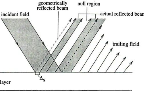
Both modified Rayleigh waves and Lamb waves are coupled as longitudinal wave to the liquid covering the acoustic waveguide. Since these modes leak back into the liquid as soon as they are excited, they are known as leaky modes [25]. Reflected field as a result of a bounded beam incidence is depicted in the following figure:

substrate

Figure 2.4: Reflected field due to the bounded beam incident at leaky wave angle

The lateral shift in the reflected field is first predicted by Schoch and it is known as Schoch displacement. A , [15] [16]. The null region is caused by the destructive interference of the specular reflection and the leaked waves.

The number of modes that is excited along the layered material depends on the shear velocities of the layer and the substrate:

a)Shear velocity of the layer is less than the substrate’s shear velocity: In this case, which is referred as loaded case, there exits modified leaky surface wave of the layer and Lamb wave modes. Figure 2.5 shows the reflection coefficient of 30 micro-meter thick aluminum layer on silicon substrate.

The right most 27t phase transition corresponds to the modified leaky Rayleigh mode of the silicon and the remaining phase transitions are the gener­ alized Lamb wave modes. If the frequency increases, more Lamb wave modes begin to appear. A new symmetric mode is added for each decrease of half longitudinal wavelength, and an antisymmetric mode for each half shear wave­ length.

Figure 2.5: Reflection Coefficient (water/al(30/z)/silicon(substrate)) at 110 MHz.

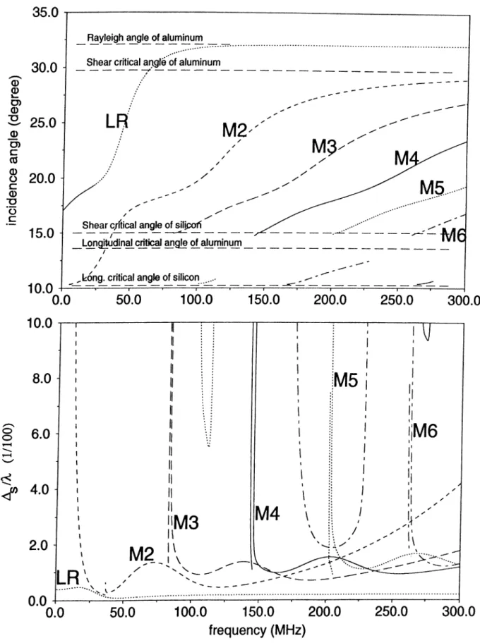
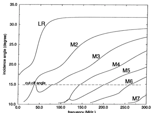
It is possible to plot frequency (or thickness) versus mode angle (or mode velocity). Graphs that are generated in this way are called as dispersion curves. Mode velocity is calculated from vm = where vm is the mode velocity, vq is the longitudinal velocity in the liquid and 6m is the mode critical angle at which the phase of the reflection coefficient is ít. Figure 2.6 contains dispersion curves for 30 micro-meter thick aluminum layer on silicon substrate loaded with water. The first observed mode is the modified leaky Rayleigh wave (LR) of the layer. The second one is the Sezawa mode (M2) which becomes pseudo Sezawa mode [5] for incidence angles below the shear critical angle of the substrate and the others axe the Lamb wave modes of the layer and the substrate. Shear critical angle of the substrate is called as cut-off angle.

Figure 2.6: Loaded Case. Dispersion Curves and Schoch Displacement of 30 micro-meter thick aluminum layer on silicon substrate.

Complex reflection coefficient has near reaJ axis pole-zero pairs, which reveal themselves as 2tt phase transitions. One way to obtain dispersion curves is to

find these poles or zeros throughout the two dimensional search of a complex kx plane. However, this is a highly computation intensive procedure, especially for high velocity modes. Local minima of the complex reflection coefficient cause problems in finding the roots. It is also possible to search for the phase transitions of the phase of the reflection coefficient, directly.

An important observation on dispersion curves is the fact that all of the modes are confined between Rayleigh and longitudinal critical angles of the layer and the substrate.

b)Shear velocity of the layer is higher than the substrate’s shear velocity,

(stiffened case): In this case there exits only one mode which is bounded to the

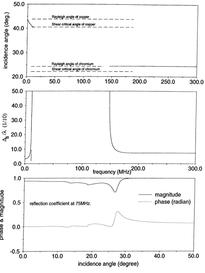
surface. For low frequencies when the wavelength in the layer is comparable to the layer thickness, it is the modified surface wave of the substrate. Rayleigh velocity of the substrate is perturbed by the layer. If the frequency is increased, wavelength in the layer becomes smaller and Surface wave velocity tends to the Rayleigh wave velocity of the layer. In figure 2.7, dispersion curve and Schoch displacements of 30 micro-meter thick chromium layer on copper substrate are shown. There is a discontinuity in the dispersion curve, and it is clear that no phase transition exists between 10 MHz and 147 MHz. Reflection coefficient at 75 MHz, in this frequency range, is also shown.

2.6

Sezaw a W aves

Dispersion curves for the loaded case are shown in figure 2.6. In this fig­ ure, second existing mode (M2) is the Sezawa mode [12]. The velocity of this mode begins at the substrate’s longitudinal velocity and eis the frequency or the thickness of the layer increases, it decreases down to Rayleigh velocity of the layer. Between longitudinal and Rayleigh critical angles of the substrate, Sezawa mode (called as pseudo Sezawa mode) has a longitudinal characteristic and leaks both to the water and the substrate. It couples to the shear wave in the substrate. This phenomenon is seen as a dip (not zero) in the reflection coefficient. For incidence angles greater than shear critical angle of the sub­ strate, mode becomes true Sezawa wave and shear in nature. It does not leak to the substrate any more and observed as 27T phase transition in the reflection coefficient.

O)

0)

0

O)

0

0

ü

ü

Shear critical angle of copper

_F^^h_an^ ^chromium_________

_ S ^ ^ c iitic a l^ ^ e of^chror^um__________

5 0 0 10O0 15Ó.0 200.0 250.0 300.0

Figure 2.7: Stiffened Case. Dispersion Curves, Schoch Displacement and Re­ flection Coefficient (at 75 MHz.) of 30 micro-meter thick chromium layer on copper substrate.

2.7

C om plex A n a ly sis o f R eflecta n ce Func­

tio n

Every linear system is characterized by special inputs that are invariant to the system. These inputs are called the eigenfunction or the modes of the system. A sound wave traveling in an acoustic waveguide is an example for linear system. Sound waves that are the solution to the acoustic boundary problem are the modes of the waveguide.

Acoustic waveguide modes can be calculated by finding the poles of the reflectance function. For every pole there exists a zero. Depending on the places of these pole-zero pairs on the complex plane, modes are observed as 2n phase transitions in the reflection coefficient. For acoustic microscopy, modes that reveal themselves as phase transitions are important and they can be observed as oscillations in V{z) curves.

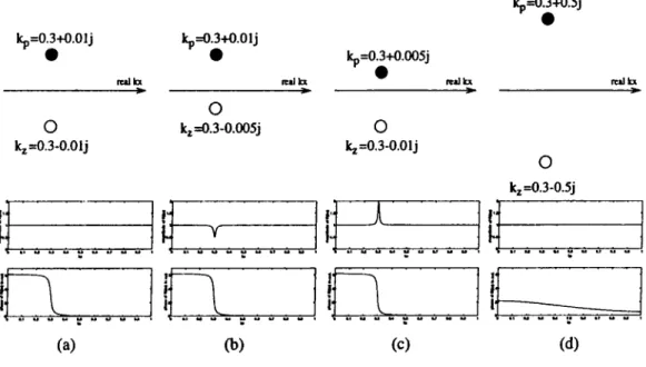
Reflectance function, in the vicinity of mode critical angles, can be approx- imated as 1Z{kx) = [11] where and kp denote complex zero and pole of the reflectance function. Figure 2.8 shows the plot of the 'JZ(kx) for real values of kx and different places of pole-zero pairs on complex plane.

kp=0.3+0.5j kp=0.3+0.01j kp=0.3+0.01j kp=0.3+0.005j real kx ^ fcal kx

o

o

o

o

X

I-

!·■

Figure 2.8: Pole-zero, magnitude and phase plot of %{kx)

In the first three figures (a,b,c) pole-zero pairs are near enough to the real axis so that they are observed as sharp phase transitions. If pole and zero are equal distance away from the axis, magnitude of 'K{kg) is 1, it is less than 1 if zero is nearer than pole and greater than 1 otherwise. In the last figure (d).

pole and zero are far away from the axis. Hence, they give rise to smooth phase variation and 2ir phase transition can not be completed in the visible space. If both pole and zero are on the same side of the real axis, their presence is observed as small phase wiggle (Figure 2.9).

kp=0.3+0.01j

O

o

O

^

1-o

Z X H

Figure 2.9: Pole-zero, magnitude and phase plot of 7Z{kx)

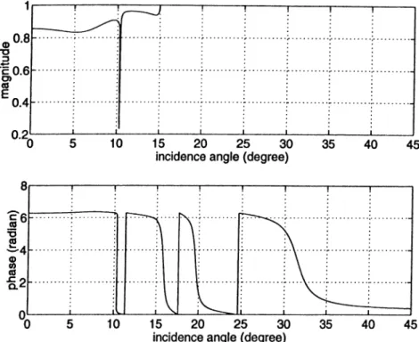
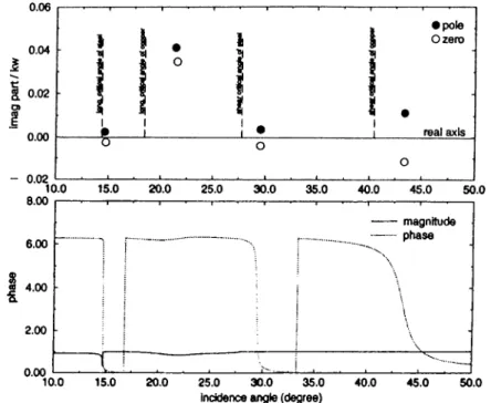
As mentioned above, poles of the reflectance function denote modal- eigenvalues. However, to observe a mode in acoustic microscopy with sufficient efficiency, corresponding pole-zero pair must satisfy certain criteria, i.e. they must be close enough to axis. In Figure 2.10 poles and zeros of the reflectance function of 400 micro-meter thick copper layer on steel substrate are shown.

8.00 6.00 4.00 2.00 10.0 15.0 20.0 25.0 30.0 35.0 40.0 45.0 50.0 0.00 magnitude phase

XT

40.0 45.0 50.0

Figure 2.10: Pole-zero plot and reflection coefficient of 400 micro-meter thick copper layer on steel substrate at 5 MHz.

Dispersion curves are calculated by finding the tt crossings of the reflection

coefficient. Hence, only observable modes are obtained. If the poles of the reflectance function is searched, all possible modes are obtained. Figure 2.11 shows the possible modes of the 30 micro-meter thick aluminum layer on silicon substrate. These curves are almost same with the previous dispersion curves for the same material combination, except some modes become unobservable below cut-off.

frequency (MHz.)

Figure 2.11: Dispersion curves for 30 micro-meter thick aluminum layer on silicon substrate. (Poles of reflectance function)

Reflectance function has many branch cuts. For single layered materials, there exists five branch cuts corresponding to the shear and longitudinal critical angles of layer, substrate and water. The sign for the propagation vectors must be chosen so as to find poles and zeros which are physically realizable. Vertical propagation vectors are calculated as:

ki,

= A- - ■

i — l,s ,w

(2.24)

where and kaz denote longitudinal and shear propagation vectors, respec­ tively. Tangential propagation vector is kx, and ¿,’s are the longitudinal or the shear complex wave numbers in the form of ^ + j a where ^ and a is the attenuation factor. For the positive values of the imaginary part of the

kx, if the real part of the kx is less than the real paxt of the A:,·, the root with

the positive real part is chosen, otherwise the root with the positive imaginary part is taken as the vertical propagation vector. For the negative values of

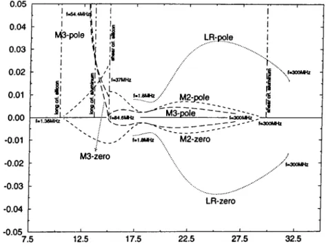
the imaginary part of the ¿x, real parts of the vertical propagation vectors are always chosen positive. Again temporal dependence is assumed. With the above arguments, branch cut is taken from + 0/^, to + io o , through to —^/,5 + io o and back to —^/,5 where 0i^s denote longitudinal or shear critical angle. This branch cut has been the standard choice both in electromagnetism and acoustics. In Figures 2.12, 2.13, 2.14 pole zero plot of the reflectance func­ tion for the loaded case (30 micro-meter aluminum layer on silicon substrate) is shown. 0.05 0.04 0.03 0.02 0.01 0.00 -0.01 -0.02 -0.03 -0.04 -0.05 . · , ^ T 1 1 bS4.4M№^ ¡ ¡ -- 1--- ---- r,--- 1---[ 1 V is ^ 3 -p o le i l ' 1 t l LR -p o le j j ... i “ ■}····... 1 El^ ' 1 ^ \l-300MH2 -cl | Ia< 1»-37MHz |l I f \\L ¡S M 2;p ole 'M 3 -p ô te ~ ~ - -_-.1^ 1-1.3«MH2 · V ^ _f-300MHz " ^ _______ ^ M 2-ze ro -M 3-zero / ,./|-300MHz LR -z e ro . 1 . 1 . 1 . 1 7.5 12.5 17.5 22.5 27.5 32.5

In the above figures, vertical and horizontal axes are the imaginary and the real parts of the tangential propagation vector, respectively. Imaginary part of the pole or zero is normalized with respect to the wave number in water and real part converted to the angle {$ = arcsin(rea/(A;a,)/¿u,)) to compare pole-zero plots with the previously given dispersion curves.

LR-pole and zero move from the Rayleigh angle of the substrate to the Rayleigh angle of the layer as the frequency increases. All other pole-zero pairs begin at the minimum of the longitudinal critical angles and tend to Rayleigh angle of the layer. There is a discontinuity across the cut-off angle. At the cut­ off, the trajectory of a pole takes it through the branch cut, it automatically passes onto an unphysical plane and a pole on the unphysical plane jump to the physical plane.

These figures do not show all poles and zeros of the reflectance function. Other poles are far away from the real axis or on the invisible space. Hence, they do not affect the phase of the reflection coefficient significantly.

If the pole-zero plots of the reflectance function of the 30 micro-meter thick aluminum layer on silicon substrate is compared with the dispersion curves (Figure 2.6) for the same material, it is seen that these graphs are in complete accordance with each other. Above cut-off all near axis poles and zeros occupy on the different sides of the real axis and they are observed as 27T phase transi­ tions. The magnitude of the reflection coefficient is 1, since the poles and zeros are in same distance from the axis. Below cut-off, for some frequency ranges,

pole-zero pairs move to the same side and their effect is as small phase wiggle on the reflection coefficient. The magnitude of the reflection coefficient is less than one, because zero is nearer than pole to the axis.

In Figure 2.15, a pole-zero pair exists below longitudinal critical angles is shown. Since, they are too close to each other and on the same side of the real axis, they vary the phase of the reflection coefficient slowly. Again, the material combination is 30 micro-meter aluminum layer on silicon substrate.

Figure 2.15: Trajectory of poles and zeros below longitudinal critical angle

In the stiffened case there exists only one near real axis pole-zero pair. The trajectory of this pair for 30 micro-meter chromium layer on copper substrate is given in Figure 2.16

2.8

Lam b W ave Lens

A wedge transducer can be used to excite leaky wave modes in a layered solid, once the frequency and the wedge angle is chosen appropriately. However, it is not suitable for imaging purposes, because of its poor resolving ability. Focusing is needed to achieve high resolution. Conical waves generated by a conical transducer or by a refraction from a suitable geometry can be an alternative for imaging. In figure 2.8 a Lamb wave lens [17] geometry which focuses conical waves to a vertical line is illustrated:

Figure 2.17: Lamb Wave Lens

The main difference between the conventional lens and the Lamb wave lens is that spherical cavity is replaced by a conical recess. The acoustic waves generated at the transducer propagate through the lens material, and refract from the top and the sides of the recess. If the inclination angle of the recess is chosen equal to the one of the mode angles, leaky wave is excited along the surface of a specimen. Reflected waves come back to the transducer after propagating in the coupling fluid and the lens.

If the envelope of the transducer’s output voltage is measured while chang­ ing the distance between lens cind the sample, one can obtain the voltage waveform as a function of distance. These curves are called V(2)’s. Typical

V{z) curves obtained from copper coated steel sample are shown in figure 2.10

and 2.11 for two different wedge angles.

(D ■D , C T j J ! 1---___________ i1___________ 1 1 10 20 30 40 in cidence an g le (d eg ree ) 50 60

Figure 2.18: Reflection CoeflBcient (water/copper(400/i)/steel(substrate)) at 5 MHz.

Figure 2.19: Simulated V{z) curve from 400 micro-meter thick copper layer on steel substrate. Lens angle=37.63°,Incidence angle=29.38°, upper radius=5.0 mm, lower radius=9.0 mm, frequency=5 MHz.

Figure 2.20: Simulated V (z) curve from 400 micro-meter thick copper layer on steel substrate. Lens angle=31.00®,Incidence angle=24.05®, upper radius=5.0 mm, lower radius=9.0 mm, frequency=5 MHz.

In figure 2.10, incidence angle coincides with the leaky wave critical angle (second existing mode in figure 2.9). Mode excitation is observed as oscillations in the V{z) curve, in the region between lens and focus, (0.0 < z < 7.5 mm). In figure 2.11, incidence angle is changed to 24.05° at which there is no mode in the reflection coefficient. So, obtained V{z) curves do not have any fringes between lens and focus.

For < {r\! idia{6incidence) ~ (^2 — r l) tau(^u,)) oscillations are due to the interference of the normal specular reflection and the non-specular reflection due to the leaky wave. The periodicity is determined by the leaky wave velocity of the particular mode and is given by:

A z = Ao

2(1 - cos(^Af)) ’ (2.25)

where &m is the critical angle of the mode. Mode velocity can be calculated by

using the following formula:

vm = Vo

s i n ( ^ A / ) ’

where vq is the acoustic velocity in the liquid.

(2.26)

In focus region, fringes cire due to the interference of the normal specular component and the oblique specular reflection. The period of the fringes is

determined by the wedge angle of the Lamb wave lens and it carries no or little information about the object. In this case periodicity is given by:

Az = Aq

2(1 COs(^,n^^dence)) (2.27)

When the incidence angle does not match with the one of the leaky wave modes, V{z) contains fringes only in focus region (Figure 2.11).

2.9

Lens D esign

Following parameters must be kept in mind while designing a lens.

Lens angle (9\v) is set such that incidence angle is one of the 27t transitions of the reflection coefficient. It can be calculated by using the following formula:

0w = 9m + arcsin sin(^H^)^ , (2.28)

where vc and u/enj are the longitudinal velocities in water and lens ma­ terial, respectively. 9m is one of the mode angle. Equation 2.28 can be

easily solved by using fix point algorithm.

Lens a p e r tu r e is determined by Schoch displacement which is calculated as

2 /a where a is the leakage rate of the mode. To probe materials with

long Schoch displacement, aperture must be wide. Schoch displacement can be also determined from the slope of the 27t phase transition.

Side w id th determines the angular bandwidth of the incident beam. It is chosen such that one of the 2w crossing is fully contained. Approximately, side width of 10 wavelength in water corresponds to 4° of bandwidth. F req u en cy also affects the angular bandwidth of the lens. As the frequency

increases while the side width is kept constant, bandwidth is decreased. So for the same bandwidth all dimensions must be decreased propor­ tionally. Frequency can be also adjusted to keep phase transition in the bandwidth of incident beam.

T ra n sd u c e r’s size must be chosen such that it insonifies all the lens aper­ ture. It’s frequency bandwidth must be wide enough to allow frequency scanning.

L en g th defines the distance between the top of the lens cavity and the trans­ ducer. To reduce diffraction losses, the top of the cavity is placed at the diffraction focus.

A sp ec t ra tio of the lens is another important parameter which defines the ratio of the lens length to the perimeter. It is kept below 0.2 to reduce background interference.

2.10

L ateral W aves

If the shear velocity of the medium is less than the longitudinal velocity of the water, it is not possible to excite leaky surface waves. In this case Lateral waves play the same role of the surface waves [11]. Lateral wave is mainly longitudinal wave propagating exactly parallel to the surface. Refraction angle is 90® and longitudinal critical angle takes place the Rayleigh angle. Hence, periodicity in V(z) is given by the formula:

A^ = Aq

2(1 — cos(^/)) ’ (2.29)

where 0i is the longitudinal critical angle of the substrate.

It is easily observed that, equation 2.13 has the value one at longitudinal critical angle.

However, it is difficult to evaluate material signature using lateral waves due to the their narrow angular width compared to the Rayleigh waves.

Chapter 3

SIMULATION

3.1

C alculation o f th e R eflection C oefficient

for th e m u lti-layered solids

The geometry of the multi layered solid [23] is shown in figure 3.1. Scalar longitudinal and vector shear potentials are denoted by (j) and respectively.

Lij and Sij are the potential amplitudes. Primary index is the number of

the layer to which the amplitude belongs. Second index denotes upward or downward propagating waves, i.e. 1 for downward and 2 for upward. With

temporal dependence, potentials can be formulated as follows:

KxX

(j)Q =

<f>i = ,

rpys = .

(3.1)

Subscript s stands for substrate. Propagation vectors, are calculated by using Pythagoras theorem. The sign of the square root must be chosen properly. For incidences below critical angles, vertical components of propaga­ tion vectors of the transmitted waves must have positive real part and above critical angles imaginary parts must be positive so that refracted waves die out with increcising values of z. Using the above arguments tangential and vertical

Figure 3.1: Geometry of a multi-layered solid

propagation vectors must be taken as:

kx = kig sin(0) ,

1

^ ^ i for k^ < ks, I jyjk'^. — kl otherwise

where 6 is the incidence angle. Wave numbers in the layers are denoted by

ki^ — ^ and kg- = ^ for longitudinal and shear waves, respectively.

Particle displacement is calculated from potentials by using the following formula: u = V<j) -f V X ^

« = (IÍÍ +

+

Longitudinal wave incidence in x-z plane can move particles only in the same plane. Particle displacement is independent of y. Hence, the second term in the divergence operation (|^ ) is zero and shear vector potential has only y component which is perpendicular to the motion plane = 0 and x¡)z = 0). After using above arguments particle displacement becomes:

U = UxX + Uyy ,

27

where , - §à ÊÉi ® ~ dx dz ' __ d4> , ay-v dz dx ' (3.5) T = c : S , _(3.6) 1 / dui d u j\ 2 ^ dxi

j

Stress tensor is given by:

where

Normal component of the longitudinal stress and the tangential component of the shear stress are calculated by using equation 3.6 and 3.7.

At fluid/solid interface, boundary conditions yield:

«Z0 = u,, , = 7;,, , 0 = 7;,, + Ty,, . (3.8) In above equation, Ty^j is also zero, since there is no displacement in y direction.

At the solid/solid boundary:

Uzi — 5 Ux^ - ) T — T T J- XZ i — ■‘■ X Z i ^ i— T

(3.9) In the case of dis-bond, tangential component of shear stress is set to zero in both medium and the continuity of the tangential displacement (ux) is no longer valid. Equation 3.9 becomes:

Uzi — 5 T ■*^zzi — ^ zzi^i Î= T T x z , = 0 , T = 0

(3.10) The number of the unknowns ‘7?, Lij., Sij' are given by ‘1 + 4n + 2’ where n is the number of layers.T’ and ‘2’ in the formula coresspond to ‘7?’ in the fluid and ‘T ,’ and ‘5 , ’ in the substrate, respectively. The number of the equations are calculated by the formula, ‘3 + 4n’, ‘3’ equations come from fluid/solid boundary and ‘4’ of them from each solid/solid boundary. Hence, there are enough equations to determine R. The simulation program evaluates these equations and solves for R using Cramer’s rule.

3.2

E ffect o f L osses in Solids

In the procedure described in previous sub-section, potentials do not contain loss terms. Since, the acoustic attenuation in metals is very low, it does not

affect the results, significantly. Typical longitudinal attenuation (a) values are 0.0040 neper/cm, 0.0049 neper/cm for aluminum and steel at 10 MHz [26]. These numbers are very low compared with that of plastics. Typical longitudinal attenuation is 0.57 neper/cm at 2.5 MHz for perspex [26]. If it is desired to calculate reflection coefficient of lossy layered solid such as epoxy

{ol/ P = 5.407 X 10"^^ neper.sec^/m yielding a = 1351 neper/m at 5 MHz) layer

on aluminum, loss terms must be included. This is easily done by adding jct term to the propagation constant. Previous k-vectors become:

—

+ ,

= ¥ + i

(3.11)

The sign of the vertical propagation constants must be chosen properly. For incidence angles less than critical angles {kx < ^ or < ^ ) , real part of k^s^

or kszi must be positive, so that refracted waves have a k-vector with a positive z component. On the other hand for greater incidence angles, imaginary part of Ar/z, or kszi must be positive to make sure that refracted waves die out as z becomes indefinitely large [27]. The direction of positive z-axis is as in the figure 3.1 and is assumed.

In figures 3.2 and 3.3 the effect of the attenuation is demonstrated. Al­ though, there exist modes in the lossless case for epoxy layer on aluminum, they vanish as the attenuation increases. In figure 3.2 longitudinal and shear attenuation constants are introduced separately. They affect the reflection coef­ ficient in the same way. Second mode, which is Rayleigh mode of the aluminum perturbed by epoxy, vanishes. In figure 3.3 shear attenuation is introduced at different levels while longitudinal one is kept constant and equal to 1351 neper/m. In this case, as the shear attenuation increases, first mode ceases to propagate.

Note that for the lossy case, magnitude of the reflection coefficient has dips near mode critical angles. Due to the non-specular reflection as mode propagates through the layer, reflected beam is shifted by A,. The reflected beam propagates a distance A, in the lossy solid, resulting decrease in the reflected amplitude.

Figure 3.2: Reflection Coefficient (water/epoxy(60/i)/aluminum(substrate)) at 5.0 MHz. Solid line indicates the case with no longitudinal nor shear attenua­ tion.

Figure 3.3: Reflection Coefficient (water/epoxy(60/i)/aluminum(substrate)) at 5.0 MHz. Longitudinal attenuation is fixed at 1351.0 neper/meter.

By investigating the pole-zero plot of the reflectance function of 60 micro­ meter thick epoxy layer on aluminum substrate at 5 MHz. for different values of longitudinal and shear attenuation coefficients, it is possible to explain dips and phcise transition of the reflection coefficient.

Figure 3.4: Pole-zero plot of the reflectance function (60 micro-meter epoxy layer on aluminum substrate) at 5.0 MHz. for different longitudinal and shear attenuation coefficients

As the longitudinal or shear attenuation coefficients are increased all poles and zeros move upward. Hence, zeros approach to the real axis. Magnitude of the reflection coefficient around critical angle becomes less than 1. If attenua­ tion is further increased zeros passes through the real axis and phase transitions do not exist any more. Only small phase variations axe observed.

Figure 3.5: Pole-zero plot of the reflectance function (60 micro-meter epoxy layer on aluminum substrate) at 5.0 MHz. for longitudinal attenuation = 5.407

X 10“^* and shear attenuation = 6.0 x 10“ *^

In above figure, all the poles and zeros are on the same side of the real axis. So, no phase transition is observed in the reflection coefficient (Figure 3.3).

3.3

C alcu lation o f D isp ersio n C urves and

Schoch D isp la cem en t

Dispersion curves give a quick overview of the modes that can be excited on the layered materials. By using these curves, immediate information is reached on the wedge angle and the operation frequency. They are plotted by finding the frequency and angle pairs at which the phase of the reflection coefficient is

7T.

Dispersion curves for the loaded single layered materials can be divided into two groups, above substrate’s shear critical angle (cut-off) and below this angle. Above cut-off, finding the tt crossings of the phase of the reflection coefficient is not difficult. Since, the dispersion curves are continuous and the phase transition is relatively slow compared to the below cut-off modes, root finding algorithm converges very fast. The root finding algorithm is implemented by using the well-known Muller method [30]. This method is very powerful and always converges in four or five iterations if good initial guesses are provided.

To find X crossings, search begins at the maximum frequency of the given frequency range in which the curves are desired to plot. First, angle intervals where the real part of the reflection coefficient is negative are found at max­ imum frequency. By using the fact that, real part of the reflection coefficient is negative around mode critical angles, good initial guesses are obtained by calculating the mid-point of these intervals. Root algorithm finds the critical angles at which the phase is x. Previous critical angles are used as initial guesses to the next step as frequency is decreased. Hence, curves are tracked beginning from the highest frequency.

Below cut-off, it is not possible to track curves, since they are discontinuous. Another difficulty arises due to the fast phase transition of these modes. So, angle v.s. frequency plane must be search two dimensionally and good initial guesses must be provided. Initial guesses are again obtained by finding the mid-point of the intervals on which the real part is negative. By using the root algorithm, critical angles are found.

Once the x crossings are found, Schoch displcicements are calculated at the critical angles by:

dR{e)

A , = 1

ko cos 9c do _0=$c (3.12)

is approximated by using 5-point formula:

f W

=

^

i m - 2h)

-

8f(e, -h) + s m + h)~ f{$,

-h 2/0].

(3.13)

where

f{6)

h

3.4

C alculation o f

V{z)

The output voltage of the transducer is ceJculated by V{z) integral [31] which relates scalar wave potential at the lens aperture to electrical output. Following figure shows the potentials (u) on the lens-sample geometry.

electrical port

- U ,

“2 Mj

Figure 3.6: Scalar potentials on the lens geometry

The scalar potential generated by the transducer of radius ’a ’ at plane-1 is given by: 1 ^ ^ a 5 ^ 0 r > a . In cylindrical coordinates: 1 r < a , 0 r > a .

Ui{x,z) = circ{\Jx^ + j/2) where circ(r) = |

u (r) =

(3.14)

(3.15)

To find potential at plane-2, Ui has to be propagated by the lens length, The angular spectrum of the potential at plane-2 can be calculated by:

U2(kr) = U i(kr)exp{-jk^l), (3.16)

kz = \J k l~ ¿2, (3.17) where kz is the propagation constant in the z-direction and ki is wave number in the lens material. Ui{kr) is the Quasi Fast Hankel Transform (QFHT) [29] of the u i(r). If cylindrical symmetry is employed, 2-D FFT can be calculated by using one dimensional QFHT. Hence, instead of u{x^ y), it is more suitable to work with u(r). Hankel and inverse Hankel transform pair is given by:

g{p) = 27t / rf{r)Jo{2'Kpr) ,

9oo

/ ( r ) = 2ir pg{p)Jo{2irpr) .

Jo

With the following variable change.

(3.18)

r = roex p (ax ), p = poexp{ay), (3.19) new functions are defined as:

9{y) = ^oe“V(^oe"*') ,

f{ x ) = roe“V(»Oe“^) , (3.20)

J{x + y) - 2πaropoe'^'^^Jo{2πaropoe^'^У) .

By replacing equation 3.20 into equation 3.18, Hankel transform pair becomes:

/ OO Λ f{ x )J { x + y)dx , -OO A f O O f { ^ ) = g{y)J{^ + y)dy · J— OO

Above cross-correlation integrals are evaluated by using 1-D FFT. In discrete time equation 3.21 corresponds to:

(3.21)

«Μ = Σ / Μ . '! * + ! / Ι .

y=0

(3.22)

In computer, U iiK ) is calculated from ui(r) by using following procedure:

/(x ) = r « i( x ) , Γ = roe“^ ,

9(y) = Σ / Η · ^ [ ^ + ί/] >

Ui{y) = i9 { y ) ^ kr= P oe^^.

where x and y are integers run from 0 to — 1 and 0 to 2N — 1. Range of y is chosen 2 times greater than that of x's to convert circular convolution to linear convolution defined in equation 3.21.

Hankel transform parameters are given by the following relations:

^0 “ ^ ’ P ^~ 1 ^ ·> ^ — · (3.24)

where /9 and b are the maximum spatial frequency and largest radial distance, respectively. Ki and K2 must be chosen such that they are greater than 2 and satisfy the following equation:

N = K 20b\n{K i^b). (3.25) In appendix C, an example for the calculation of Hankel parameters is given.

After finding U2{K) by using equation 3.16, scalar potential U2{r) is cal­

culated by employing inverse Hankel transform. Potential at plane-2 is passed through the conical recess by using ray theory. Referring to the figure 3.6, potential distribution at the front of the lens is given by:

U3(r) = where tt2(r)exp(j>Â:2dı) 0 < r' < r l , \j^^ARU2{r')exY>{j{kidi -f ¿2^2)) r l < r' < r2 , 0 r2 < r ' , Ar = -f tan tan(0,i,_a) , (3.26) r' = (3.27)

r + T2 tan 6yj ta,n{6,u — a) 1 -|- tan 0tu tan(0,i, — a) ’

a = arcsm — sm ) ,

V^2

J

dl = (r' — rıjtanûu) , d2 = (r2 - r ') — -7 .

cos(0u, — a)

Figure 3.7 depicts the potentials at the transducer plane and at the back of the conical recess. Transducer radius is 6.5 mm, upper and lower radii of the recess are 2.5 mm and 5.0 mm, respectively. Maximum radial distance is chosen as 10.0 mm. Figure 3.8 shows the angular distribution at the lens aper­ ture. Wedge angle is 40.0*^ which gives the incidence angle of 31.3°. Operation frequency is 5 MHz.

Finally, output voltage is given by the integral of the multiplication of the downward (t/si^r)) and upward propagating fields {U3{kr)1l{kr)e^^''‘^) at

the aperture, where TliK) is the reflection coefficient and phase term corresponds to two way distance between lens and sample surface. Voltage integral:

>=rk.Vi(K)-R{K)U3(K) exp{j2k,z)dkr (3.28) where P is the incident power at the transducer’s terminals and / stands for frequency. Integral formula is calculated by using the trapezoidal approxima­ tion.

0 0.001 0.002 0.003 0.004 0.005 0.006 0.007 0.006 0.009 0.01 radial distance (meter)

Figure 3.7: Magnitude of potentials at plane-1 and plane-2.

Chapter 4

V { z )

RESULTS FROM HIGH

VELOCITY MODES

High velocity modes refer to Lamb waves that exist below the shear critical angle of the substrate, when it is loaded by a layer whose shear velocity is less than substrate’s shear velocity. The velocity of these modes are higher than both layer and substrate’s shear velocities. This family of modes heis some useful characteristics in the examination of layered materials. In this chapter, the effect of the bond quality on V(z) curves obtained from specially prepared sample is investigated by using above cut-off modes cind high velocity modes.

4.1

E x p erim en ta tio n

Electronic setup that is used to obtain V{z) data is depicted in figure 4.1. The setup consists of lens, amplifiers, switches, signal and pulse generators and a computer which controls the 2 drive. Signal generator provides sinusoidal waveform which is gated by transmit (T) switch with a pulse width of 2 /usee for operation at around 32 MHz. Hence, one sine burst nearly contains 60 cycles at 32 MHz which is enough to simulate continuous sine wave. Then, sine burst is amplified by an amplifier with gain of 30-dB. Resulting signal is again gated by transmit/receive (T /R ) switch and pumped to the lens. T-switch and T/R - switch are controlled by the same clock. They transmit at the same time. In the receive timing, only desired part of the reflected echoes is gated by the third switch (R-switch) and amplified by an amplifier and output waveform is observed on CRT screen. Negative peak detector detects the envelope of

the sine burst and while computer controlled step motor scans z axis, output voltage is measured via averager and multimeter. Multimeter output is read by the computer and recorded.

Pulse repetition rate (PRR) must be chosen such that it allows return echoes to die out and it should be high to increase signal to noise ratio. A suitable PRR is found as 10 kHz. PRR is set by synchronization circuit by converting 1 MHz sine wave, obtained from signal generator, to square wave and dividing it. Frequency divider consists of T T L decade counters. By taking the output from different counters desired PRR is obtained.

Although, all electronics part have nearly 1 GHz bandwidth (4 MHz-1 GHz), actual bandwidth of the microscope is determined by the transducer which has ±2.5 MHz bandwidth around 32 MHz.

Figure 4.1: Electronic setup

Transducer is coupled to the lens by phenyl salicylate (salol) as described in reference [32], pages 259-261.

4.2

V{z)

R esu lts

Experimental and simulated V (z) curves for good and dis-bond cases are shown in figure 4.2. The wedge angle is 45.5° and corresponding incidence angle is 35.85°, which is higher than the cut-off angle of steel (28°). In good bond case the existence of above cut-off mode is observed as fringes between lens and focus. In the dis-bond case, mode critical angle is shifted and incidence angle does not match with the critical angle. Hence, fringes are due to the geometrically reflected beams and exist only in focus.

Figure 4.2: Calculated and experimental V{z) from 500 micro-meter copper on steel substrate. Operation frequency is 6.65 MHz. Upper radius=3.91 mm Lower radius=5.95 mm

Figure 4.3 shows the reflection coefficient of 500 micro-meter thick copper layer on steel half space for good bond and dis-bond cases. For the good bond case, there exists a high velocity mode at 15.30®. In figure 4.4 theoretical V{z) curves obtained by a lens whose incidence angle coincides with this angle are shown. Solid and dotted lines coresspond to good bond and dis-bond cases, respectively. Wedge angle is 20.0®, upper and lower radii of the lens are 6.0 mm and 12.0 mm. Operation frequency is chosen as 32 MHz. In the case of dis-bond, mode no longer exists. However, small variation in the phase gives rise to small fringes in V{z).

incidence angle (degree)

Figure 4.3: Reflection Coefficient of 500 micro-meter thick copper layer on steel substrate for good bond and dis-bond cases at 32 MHz.

0.000 0.040

Figure 4.4: Calculated V(z) from 500 micro-meter copper on steel substrate for good bond and dis-bond cases at 32 MHz.

The lens used in above simulation is very large, by using small lenses it is still possible to differentiate good and dis-bonds. In figure 4.5, theoretical and experimental V{z) curves from the same sample are shown. Solid lines and dots correspond to calculated and experimental data, respectively. Upper and lower radii of the lens are 1.75 mm and 3.50 mm. In both cases a good agreement is observed between computed and measured data. It is possible to recognize the bond type by measuring the amplitude of the fringes due to the leaky waves. The amplitude of the fringes in good bond case is greater than that of dis-bond case.

Although, it is possible to excite high velocity modes with a Lamb wave lens, there are some difficulties. Since, the angular width of the phase transition is very narrow, lens must be manufactured with great care. Small errors in the wedge angle result in wrong incidence angles and mode may not be excited.