Monte Carlo simulation of electron transport in degenerate and inhomogeneous semiconductors

(1)

Monte Carlo simulation of electron transport in degenerate and inhomogeneous

semiconductors

Mona Zebarjadi, Ceyhun Bulutay, Keivan Esfarjani, and Ali Shakouri

Citation: Appl. Phys. Lett. 90, 092111 (2007); doi: 10.1063/1.2709999 View online: http://dx.doi.org/10.1063/1.2709999

View Table of Contents: http://aip.scitation.org/toc/apl/90/9

Published by the American Institute of Physics

Articles you may be interested in

Improved Monte Carlo method for the study of electron transport in degenerate semiconductors

Journal of Applied Physics 84, 3706 (1998); 10.1063/1.368547

Tunneling-assisted Poole-Frenkel conduction mechanism in thin films

Monte-Carlo-based spectral gain analysis for terahertz quantum cascade lasers

Modeling of electron–electron scattering in Monte Carlo simulation of quantum cascade lasers

The Three-Dimensional Poole-Frenkel Effect

The Poole-Frenkel Effect with Compensation Present

(2)

Monte Carlo simulation of electron transport in degenerate

and inhomogeneous semiconductors

Mona Zebarjadia兲

Department of Electrical Engineering, University of California, Santa Cruz, California 95064

Ceyhun Bulutay

Department of Physics, Bilkent University, Ankara 06800, Turkey

Keivan Esfarjani

Department of Physics, University of California, Santa Cruz, California 95064

Ali Shakouri

Department of Electrical Engineering, University of California, Santa Cruz, California 95064

共Received 14 November 2006; accepted 26 January 2007; published online 28 February 2007兲 An algorithm is proposed to include Pauli exclusion principle in Monte Carlo simulations. This algorithm has significant advantages to implement in terms of simplicity, speed, and memory storage; therefore it is ideal for the three-dimensional device simulators. The authors show that even in moderately high applied fields, one can obtain the correct electronic distribution. They give the correct definition for electronic temperature and show that in high applied fields, the quasi-Fermi level and electronic temperature become valley dependent. The effect of including Pauli exclusion principle on the band profile, electronic temperature, and quasi-Fermi level for the inhomogeneous case of a single barrier heterostructure is illustrated. © 2007 American Institute of Physics. 关DOI:10.1063/1.2709999兴

Many of today’s interesting microelectronic devices are working in high doping concentrations up to 1020_cm−3_.

De-generate semiconductors are important for thermoelectric and thermionic energy conversion devices and they are also used in the highly doped source/drain regions of advanced transistors. At high carrier densities, the electron distribution is highly affected by its fermionic nature. Therefore, Pauli exclusion principle共PEP兲 needs to be included in the theo-retical analysis of electron transport in degenerate semiconductor-based structures.

If the electron wavelength is smaller than the character-istic lengths present in the structure, the Boltzmann transport equation 共BTE兲 can be used as an appropriate governing equation for the device. The factor 共1− f兲 in BTE, which indicates the probability of the final state to be unoccupied, is present in the scattering term as a result of PEP.

⳵f共r,k,t兲 ⳵t = − v ·⵱f共r,k,t兲 − F/ប · ⵱kf共r,k,t兲 +

兺

k⬘ 兵W共k

⬘

,k兲f共r,k

⬘

,t兲关1 − f共r,k,t兲兴 − W共k,k

⬘

兲f共r,k,t兲关1 − f共r,k

⬘

,t兲兴其.

Here, f is the nonequilibrium distribution function, F is the applied electric force, v is the group velocity, and W the scattering rate. The ensemble Monte Carlo共MC兲 simulation is accepted as a powerful numerical technique to solve BTE and is widely used to simulate transport in semiconductor devices. There have been some attempts to include PEP in MC simulations of degenerate semiconductors. All of these attempts have been based on the rejection method. At each scattering step, scattering to the final state is accepted with

the probability of 1-f. However, in a MC simulation f is not

a priori known.

In a single-electron MC simulation Bosi and Jacoboni1 suggested using f共k,t兲 obtained from the simulation itself up to the time t at which the scattering is attempted. They evalu-ate f共k,t兲 on a grid in k-space. Lugli and Ferry2 _共LF兲 pro-posed using the same method in ensemble MC simulation, but substituting the averaging over time by ensemble average at each time step. This algorithm is working well at high fields but it is not suitable for low fields and highly degen-erate cases. In low fields, it is reported that the algorithm leads to some unphysical results such as the decrease of av-erage electron energy with the increase of electric field and values of electron distribution function exceeding 1.3 In or-der to improve the LF method, Borowik and Thobel3 and Borowik and Adamowicz4 suggested adding scattering-out terms into the simulation by introducing virtual scatterings in order to avoid f⬎1. With this method they were able to rebuild the Fermi-Dirac distribution with a small deviation. We believe that in principle LF method is free from these artifacts at the cost of excessive k-space grid points, also implying a large number of simulated particles. Besides, if PEP is also checked after free flights, the distribution func-tion should not exceed 1.5Another inconvenience of the LF method is that this algorithm is suitable for a homogeneous steady state situation. In transient simulations and in inho-mogeneous devices, tabulating the distribution function at various locations and times can require an unmanageable computation time and storage.

Fischetti and Laux6proposed to overcome this difficulty by approximating the local electron distribution by a quasi-equilibrium Fermi-Dirac distribution with the following defi-nition for local electronic temperature:

a兲_{Electronic mail: mona@soe.ucsc.edu}

APPLIED PHYSICS LETTERS 90, 092111共2007兲

(3)

3

2kBTel共r兲 =

再

具E共r兲典 nondegenerate

␮共r兲 degenerate,

冎

共1兲 where␮共r兲 is the local quasi-Fermi level and 具E共r兲典 is the local average kinetic energy of electrons. The above defini-tion for electronic temperature is not correct at high concen-trations when the Maxwell-Boltzmann distribution is not valid. The correct definition of electronic temperature should converge to the lattice temperature at zero electric field and should exceed it under an applied field. Moreover, under the applied bias, translational energy should be subtracted, be-cause temperature is defined by fluctuations of electron ve-locities around its mean drift value. These considerations lead us to the following definitions for the distribution func-tion and electronic temperature of each valley:

fv共E,␮v,Telv兲 = 1 exp共关Ev共兩k − kd v_{共r兲兩兲 −}_␮ v共r兲兴/kBTelv共r兲兲 + 1 , 共2兲 T_elv共r兲 = 2 3kB 共具Ev共k − kd v_{共r兲兲典 − 具E} v共r兲典0兲 + Tlattice. 共3兲

Herev is the valley index, and具Ev共r兲典0 is the local average

energy of electrons in equilibrium at zero electric field and is calculated analytically at each time step关see Eq.共5兲兴. kdv共r兲

is the local drift wave vector, which is the average wave vector of all the particles at position r and in valleyv. For

moderately high field electrons in different valleys are not in equilibrium with each other, so separate Fermi spheres with different chemical potentials and temperatures need to be defined for each valley. Therefore, all quantities are valley dependent. Also in inhomogeneous cases such as hetero-structures, we need to discretize the x space and define the Fermi level and the electronic temperature locally.

The implementation of the algorithm in the MC simula-tion is straightforward. At each time step, the drift wave vec-tor共kd兲, average energy of electrons 共具E共k−kd兲典兲, and local

charge 共n_cv兲 are calculated. Then electronic temperature, Fermi level, and 具E_v典₀ for each valley can be calculated, using Eqs.共3兲–共5兲, respectively.

nc v =

冕

−⬁ ⬁ f共␧,␮v,Tel v_兲g v共␧兲d␧, 共4兲 具Ev共r兲典0=

冕

−⬁ ⬁ 共␧ − ␧c v_兲f共␧,_␮ v共r兲,Tlattice兲gv共␧兲d␧, 共5兲

where gv共␧兲 is the density of states and ␧cvis the bottom of

the conduction band in the valley␯. These updated quantities are used in Eq.共2兲for scattering probabilities into final states at the next iteration.

Figure1 shows the distribution function at zero electric field obtained from the present algorithm in comparison with analytical Fermi-Dirac 共FD兲 distribution. The deviation is negligible in most of the energy range. However, using defi-nitions of Ref.6 关Eq. 共1兲兴, the obtained final distribution is

totally different from the FD distribution. It also shows the results of implementing the algorithm with a low applied field. As expected some of the electrons below Fermi level are pushed to higher energy levels producing thereby heating.

Figure2shows a comparison between our algorithm and experimental results.7The experiment has been done at 77 K on Te-doped GaAs. In low temperatures, impurity scattering is the dominant scattering mechanism. In this simulation, we have included both ionized and neutral impurity scatterings. Neutral impurities are considered as hard spheres with the potential of 35 eV and radius of 2 Å. A binding energy of 0.03 eV is considered for tellurium in GaAs.8 Polar optical and acoustic phonons are also included, both as inelastic pro-cesses. Although there is some deviation compared to experi-mental results, our results are closer to the experiment com-pared to the previous work of Ref.1.

In Fig. 3we compare the distribution function obtained from our suggested algorithm with that of the LF method. Scattering rates and band structure are the same for both cases and the only difference is the implementation of PEP. The agreement between the present method and the LF method suggests that the present algorithm works very well even at moderately high fields of the order of several 10 kV/ cm. Our modeling 共nonparabolic multivalley band structure兲 becomes questionable at such fields for GaAs, so this should only be considered as a confirmation of the va-FIG. 1. 共Color online兲 Electron energy distribution function at equilibrium for GaAs at room temperature and the doping of 1019_cm−3_{. Theoretical}

Fermi-Dirac function is plotted for comparison. The rest are Monte Carlo simulation results implementing共a兲 present algorithm, 共b兲 algorithm of Ref.

6关Eq.共1兲兴, and 共c兲 without Pauli exclusion principle. The last data are the

result of present algorithm for low applied electric field of 2 kV/ cm.

FIG. 2. Relative change of the electronic distribution to the equilibrium共FD distribution兲 at 77 K temperature and the doping density of 5⫻1017_cm−3_.

Experimental results共solid curve兲 are after Ref.8. MC data obtained from our simulation for the same applied electric fields 共200, 400, 600, and 900 V / cm from top to bottom兲 are shown by dotted lines. Previous MC simulation results of Ref.1are shown by dots共at 900 V/cm兲.

(4)

lidity of our method and not a quantitative prediction of the electronic distribution at high fields. The figure is plotted for high doping of 1019cm−3. In such a high doping, the LF method gives reasonable results with at least 700 000 elec-trons 共this large number of electrons is essential for repro-ducing the correct results especially at low fields兲; however, the present method is working well even with a sample of 10 000 electrons implying a reduction in CPU time and memory by a factor of 70! Moreover, even with the same number of electrons the LF method uses 4.7 times the memory and it is 15% slower in comparison with the present method. These simulations were done on a personal com-puter with Pentium共R兲 4 processor and 2.0 Gbytes of memory. It is noticeable that the agreement with the LF method, at high fields, is obtainable only if the quasi-Fermi level is defined separately for each valley.

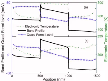
Finally, we applied this approach to the inhomogeneous case of a single barrier heterostructure. In the absence of bias 共equilibrium case兲 the quasi-Fermi level is constant through-out the whole device. Withthrough-out considering PEP, however, the distribution would not lead to a constant Fermi level. Figure

4 shows the electronic temperature and quasi-Fermi level under a low applied bias, with and without applying PEP. The simulation is at room temperature. Without PEP, elec-trons are much colder than the lattice temperature especially in the contact layers where Fermi level is within the conduc-tion band. In this case electrons would go from the barrier to the lower occupied states in the contacts and overpopulate them. This would lead to an artificial band bending which is shown in Fig.4. By including degeneracy in the calculation, distribution leads to a continuous Fermi level and the elec-tronic temperature is close to the lattice temperature. Cooling of electrons before the barrier and heating of them after the barrier can be explained as Peltier cooling and heating, and heating inside the barrier is a result of Joule heating. The transition between nonlinear thermionic emission cooling

and linear transport is discussed in a recent publication.9We need to add that the irregularities at both ends of the sample stem from the injection mechanism imposed at the bound-aries. They would become irrelevant for wider contact regions.

In summary, we proposed a theory which describes with good accuracy transport in degenerate and inhomogeneous semiconductors. It was shown that the algorithm requires much less time and memory storage compared to LF and similar methods. This allows the treatment of inhomoge-neous systems, which is almost an impossible task with the LF method; therefore it is ideal for the three-dimensional device simulators. We have also given a definition for the electronic temperature, which leads to the correct distribu-tion funcdistribu-tion in good agreement with these methods. Com-parisons with analytical results at zero bias and with other algorithms and also experimental data under applied bias were also presented. Furthermore, the effect of including PEP in a heterostructure on the band profile, electronic tem-perature, and the quasi-Fermi level was illustrated. The theory correctly predicts a continuous electronic temperature profile and quasi-Fermi level across the junctions.

One of the authors共M.Z.兲 is thankful to U. Ravaioli for helpful discussions. The authors also wish to acknowledge the support by ONR Thermionic Energy Conversion Center MURI.

1_{S. Bosi and C. Jacoboni, J. Phys. C 9, 315}_共1976兲.

2_{P. Lugli and D. K. Ferry, IEEE Trans. Electron Devices 32, 2431}_共1985兲. 3_{P. Borowik and J. L. Thobel, J. Appl. Phys. 84, 3706}_共1998兲.

4_{P. Borowik and L. Adamowicz, Physica B 365, 235}_共2005兲.

5_{P. Tadyszak, F. Danneville, A. Cappy, L. Reggiani, L. Varani, and L. Rota,}

Appl. Phys. Lett. 69, 1450共1996兲.

6_{M. V. Fischetti and S. E. Laux, Phys. Rev. B 38, 9721}_共1988兲. 7_{W. Jantsch and H. Bruker, Phys. Rev. B 15, 4014}_共1977兲.

8_{S. M. Sze, Semiconductor Devices, Physics and Technology}_{共Wiley, New}

York, 1985兲.

9_{M. Zebarjadi, A. Shakouri, and K. Esfarjani, Phys. Rev. B 74, 195331}

共2006兲. FIG. 3. 共Color online兲 Comparison between LF method and the present

method: distribution function for three different applied electric fields. Solid lines are obtained from the present algorithm and dots are obtained from LF method. For more clarity, the three graphs are shifted upwards by two units, and different valley minima are shown with an arrow.

FIG. 4. 共Color online兲 Band profile, quasi-Fermi level, and electronic tem-perature for InGaAs/ InGaAsP / InGaAs heterostructure at room temtem-perature under a low applied bias共a兲 without and 共b兲 with PEP. Note that in 共b兲 they are continuous across the junctions.