Simulation metamodeling with neural networks

SIMULATION METAM bDELING WITH NEURAL

NE*iW0RKS

A THESIS

SUBMITTED TO THE DEPARTMENT OF INDSTRIAL

ENGINEERING

AND THE INSTITTE OF ENGINEERING AND SCIENCES

OF BILKENT UNIVERSITY

IN PARTIAL FULFILMENT OF THE REQUIREMENTS

FOR THE DEGREE OF MASTER OF SCIENCE

Souheyl Touham i

June, 1997

SIMULATION METAMODELING WITH NEURAL

NETWORKS

A THESIS

SUBMITTED TO THE DEPARTMENT OF INDUSTRIAL ENGINEERING

AND THE INSTITUTE OF ENGINEERING AND SCIENCES OF BILKENT UNIVERSITY

IN PARTIAL FULFILLMENT OF THE REQUIREMENTS FOR THE DEGREE OF

MASTER OF SCIENCE

By

Soiiheyl Toiihcimi

June, 1997

C'/.·

I certify that I have read this thesis and that in my opinion it is fully adequate, in scope and in quality, as a thesis for the degree of Master of Science.

— . t

Assoc. Prof. Ihsan Sabuncuoğlu(Principal Advisor)

I certify that I have read this thesis and that in my opinion it is fully adequate, in scope and in quality, as a thesis for the degree of Master of Science.

Assoc. ProfT Osman Oğuz

I certify that I have read this thesis and that in my opinion it is fully adequate, in scope and in quality, as a thesis for the degree of Master of Science.

Assoc. Prof.^Omer Ivlorgiil

Approved for the Institute of Engineering and Sciences;

Prof. Mehmet ^^^ly

ABSTRACT

SIMULATION M ETAM ODELING W ITH NEURAL

NETW ORKS

Souheyl Toiihami

M.S. in Industrial Engineering

Supervisor: Assoc. Prof. Ihsan Scibuncuogiu

.June, 1997

Modern manufacturing environments increasingly call for more sophisticated

cind fast decision aiding systems for their management. Artificial neural

networks have been proposed as an alternative cipproach for formalizing various quantitative and qualitative aspects of manufacturing systems. This research attempts to lay down the motivation behind using neural networks

as a simulation metamodeling approach. This research can be classified

under the major headings of simulation metamodeling for the purpose of estimating system performance. Steiidy state perfornuince of non-terminating type systems and transient state performance of terminating tyj^e systems are examined under job shop environments by applying Back Propagation neural networks. We attempt to study the peribrrnance of neural metamodels with respect to estimating two performance measures (mean machine utilization and mean job tardiness), with respect to system complexity, with different types of system configurations (deterministic cuid stochastic), with respect to multiple metamodel accuracy assessment criteria and various metamodel design settings. The objective of this analysis is to investigate the potential application of neural metamodeling.

K ey words: Simulation, Metamodeling and Neural Networks.

ÖZET

YA P A Y SİNİR AĞLARI İLE BENZETİM M ETA

MODELLERİNİN OLUŞTURULMASI

Souheyl Touhami

Endüstri Mühendisliği Bölümü Yüksek Lisans

Tez Yöneticisi: Dr. Ihsan Sabuncuoğlu

Haziran, 1997

Günümüzde modern imalat sistemleri daha karışık ve hızlı karar veren yöntemlere ihtiyaç duymaktadır. Bu amaca yönelik olarak, yapay sinir ağları cdternatif yöntem olarak önerilmektedir. Bu çalışmada, yapay sinir ağlarının bu tür yöntemlerde kulicinılmalarmı sağlayacak temeller oluşturulmaktadır. Gerek uzun dönemli ve gerekse kısa vadeli sistem performansını ölçecek

modeller oluşturulmaktadır. Geri yaymalı (back propagation) yöntemine

dayalı olarak geliştirilen yapay sinir ağları sistemin ortalama kullanım oranı ve artı gecikme zamanı performans ölçütlerini tahmin etmekte kullanılacaktır. Önerilen yakalaşım ve geliştirilen modellerin başarısı çeşitli sistem koşullarında farklı değerlendirme kriterine göre ölçülecektir.

Anahtar sözcükler: Benzetim, Meta modellemesi, Yapay Sinir Ağları

ACKNOWLEDGEMENT

I would like to express my deep gratitude to Dr. Ihsan Sabuncuoğlu for his guidance, attention, understanding and patience throughout all this work. I am indebted to the readers Dr. Osman Oğuz and Dr. Oiner Morgiil for their effort, kindness, and time.

I cannot fully express my gratitude and thanks to my friends for their care, support and encouragement.

Souheyl Touhami.

Contents

1 Introduction 1

2 Research Background 4

2.1 S im ulation... 4

2.2 Simulation M etam odels... 7

2.3 Neural Networks 10

2.4 Neural networks as a simulation rnetamodeling approach . . . . 19

3 Estimating Long Term Machine Utilization 25

3.1 Case 1: Simple S y s t e m ... 26

3.1.1 Experimental settings... 26

3.1.2 Results and Discussions 33

3.2 Case 2: Complex S y s te m ... 36

3.2.1 Experimental settings... 37

3.2.2 Results and Discussions 40

3.3 Comparison of Simple vs. Complex systems 42

CONTENTS VHl

4 Estimating Long Term Job Tardiness 44

4.1 Case 1: Simple S y s t e m ... 45

4.1.1 Experimental settings... 45

4.1.2 Results and Discussions 51

4.2 Case 2; Complex S y s te m ... 55

4.2.1 Experimental .settings... 55

4.2.2 Results and Discussions 57

4.3 Compcirison of Simple & Complex s y s t e m s ... 59

5 Estimating Short Term Job Tardiness 62

5.1 Experimental settings... 63

5.2 Results and Discus.sions 66

6 C O N C L U D IN G R E M A R K S 74

A Figures 85

B Tables 98

List of Figures

2.1 Metamodeling Concept. 9

2.2 The generic network architecture used... 12

2.3 Single processing unit in neural network... 13

3.1 Mean Utilization: Simple System: Relationship between models. 28

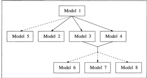
3.2 Mean Utilization and Mean Tardiness: Complex System:

Relationship between models... 38

4.1 Mean Tardiness: Simple System: Relationship between models. . 47

5.1 Mean Tcirdiness: Simple System: Short term performance

estimation: Relationship between Metamodels... 65

3.1.2 Mean Utilization: Metaniodel performiince through assessment

criteria. 86

3.1.3 Learning curve for selected best neural network... 87

3.2.2 Mean Utilization: Complex System: Metamodel performance

through assessment criteria... 88

3.3 Mean Utilization: Comparisons... 89

LIST OF FIGURES

4.1.2 Mean Tardiness: Simple System: Metamodel performance

through assessment criteria... 90

4.2.1 Mean Tardiness: Complex System: Metamodel performance

through assessment criteria... 92

4.3 Mean Tardiness: Compaihsons... 94

5.2 Mean Tardiness: Simple System: Short term performance

estimation: Metamodel performance through assessment criteria. 95

5.3 Mean Tardiness: Short term performance estimation: Compar­

ing effect of stochasticity and system complexity. 97

2.1 Metaniodeling Concept. 9

2.2 The generic network architecture used... 12

2.3 Single ¡:)rocessing unit in neural network... 13

3.1.1 Mean Utilization: Simple System: Relationship between models. 28

3.1.2 Mean Utilization: Metaniodel perforniiuice through assessment

criteria. 28

3.1.3 Learning curve for selected best neural network... 28

3.2.1 Mean Utilization and Mean Tardiness: Complex System:

Relationship between models... 38

3.2.2 Mean Utilization: Complex System: Metamodel performance

through assessment criteria... 28

3.3 Mean Utilization: Comparisons... 28

LIST OF FIGURES XI

4.1.2 Mean Tardiness: Simple System: Metamodel performcince

through assessment criteria... 47 4.2.1 Mean Tardiness: Complex System: Metcimodel performance

through assessment criteria... 47

4.3 Mean Tardiness: Comparisons... 47

5.1 Mean Tardiness: Simple System: Short term performance

estimation: Relationship between Metamodels... 65

5.2 Mean Tardiness: Simple Sj^stem: Short term performance

estimation: Metamodel performance through assessment criteria. 65

5.3 Mean Tardiness: Short term performance estimation: Compar­

List of Tables

3.1.1 Mean Utilization; Simple System: List of inocleL

99

3.1.2 Mean Utilization: Simple System; List of neural metamoclels.. . 99

3.1.3 Mean Utilization: Simple System: Results of metamodels. . . . 100

3.1.4 Error report of Pierreval’s network...102 3.1.5 Robustness test... 102

3.2.1 Mean Utilization: Complex System: List of models... 103

3.2.2 Mean Utilization: Complex System; Generated set characteristics. 103

3.2.3 Mean Utilizcition: Complex System: List of neural metamodels. 104

3.2.4 Mean Utilization: Complex System: Results of metamodels. . . 105

4.1.1 Mean Tardiness: Simple System: List of models. 109

4.1.2 Mean Tcirdiness; Simple System: Generated set characteristics. . 109

4.1.3 Mean Tardiness: Simple System: List of neural metamodels. . . 110

4.1.4 Mean Tardiness; Simple System: Results of metcimodels...112

4.2.1 Mean Tardiness: Complex System: List of models... 120

LIST OF TABLES Xlll

4.2.2 Mecin Tardines.s: Complex System: Generated set characteristics. 120 4.2.3 Mean Tardiness: Complex System: List of neural metamodels. . 121 4.2.4 Mean Tardiness: Complex System: Results of metamodels. . . . 122

5.1 Mean Tardiness: Short term estimation: List of models...126

5.2 Mean Tardiness: Short term estimation: Generated set

characteristics... 127

Chapter 1

Introduction

Simulcition has been widely accepted by the OR community ¿uid the business sector as a valuable tool in solving large problem instances that are unsolvable (or expensively solvable) with other quantitative approaches. However, due to the time requirements and lack of optimization capabilities, simulation may not be appropriate lor real time cipplications, which are more and more calling for faster techniques. The use of simulation metamodels may help solve such problems. Research in metamodeling is maturing. Since 1987, a resurgence of interest mostly appears as case studies. This is the case also for use of neural networks as a metamodeling approcich, which cire quite recent. The case studies reported in the literature are not elaborated enough to allow assessing their potential applications in real life.

The aim of this work is to investigate the boundaries of simulation metamodeling with Artificial Neural Networks for the purpose of estimating system performance measures in job shop environments. This study is based on neural networks that operate with the Bcick Propagation algorithm. This reseiirch htvs two major parts. In the first part, we evaluate the performance of the neural networks in estimating long term or steady stcite performance of non- termiiiciting type simulations. We attempt to determine the effect of system performance measures (mean job tardiness vs. mean machine utilization), system configuration (deterministic vs. stochastic), system complexity (simple

CHAPTER 1. INTRODUCTION

vs. complex), error assessment criteria and network design settings on the predictive capabilities of the designed neural metamodels. In the second part, we evaluate the neural networks in estimating short term or transient state system performance with terminating type simulation. In this latter part, the initial system status plays an important role. For this we investigate the effect of the initial system status, demand on system, error assessment criteria and network design settings on the predictive capabilities of the designed neural metamodels. A simulation investigation of a pcirticular system might be either terminating or non-terminating, depending on the objectives of the study. The terminating tyjDe simulation is one for which there is a “natural” event that specifies the length of the simulation run and the nonterminating type is the one for which there is no such event. In our experiments, we assume that the objective of the study is to the evaluate the long term cuid short term impact of the selected operiitional policies cind hence we assume that the ending event for the terminating simulation is imposed by the management and is specified in terms of time. For the non-terminating simulation, simulation run lengths are set as to reveal steady state system behavior.

It has not been of primary emphasis for us to find the best (most precise) neural network metamodel for each of the systems that are studied. Therefore, all the results achieved could be improved through further fine tuning of the experiments. However, we believe that these improvements will not alter the conclusions inferred from this work. The results achieved in the experiments show that neural networks are very promising tools for estimating steady state system performance. For estimating short term system performance, the experiments show that it is a more difficult task and we stiite some of the factors that influence the performance of neural networks. The experiments indicate that, although neural networks are promising, application to real life may not be straight forward as the existing literature may lead us to expect.

This manuscript consists of 6 chapters. The next chapter lays down the

background of our research. The next two chapters are under the major

heading of simulation metamodeling with neural networks of non-terminating

CHAPTER 1. INTRODUCTION

utilization. The fourth chapter is related to predicting mean job tardiness. The fifth chapter reports the work done on simulation metamodeling with neural networks of terminating type systems. In the last chcipter we give our conclusions and future research directions. All the related tables, figures and graphs related to this work are provided in the Appendices.

Chapter 2

Research Background

2.1

Simulation

Considering the inherent complexities in modern manufacturing, it is of prime importance for modern management to quickly evaluate the impact of their oj^erational policies on the overall short term and longer term performance of the system before actual implementation takes place, in order to keep up with the dynamic nature of modern business. Thus, the ancilysis tool used must be fast cind with an acceptable degree of precision [12]. When analytical methods can be employed, they can generate the best model of a system. However, due to the strict assumptions required on system states and the complex and lengthy mathematical derivations involved, many analytical models cannot be applied to large or complex systems. Computer simulation is frequently used in these circumstances as an alternative solution approach to solve such problems.

Simulation is a key decision making tool in an advanced manufacturing environment. It reduces the cost, time and risks compared to experimenting

decision alternatives with real systems in real time. Simulation allows

evaluating short term and long term effect of decision made cit all the levels

of the manufacturing system. Either used at the system design phase or

when operating the system, simulation is a flexible system analysis tool that

CHAPTER 2. RESEARCH BACKGROUND

allows modeling relatively large systems without requiring many restrictive assumptions. It is used where other approaches find it difficult in terms of modeling and computational recpiirements [31]. Thus, it is a complementary tool and not in competition with other approaches. Simulation is applicable at all the levels of the hierarchical decision making process, allowing to perform sensitivity analysis and to evaluate different policies at different degrees of aggregation under selected experimental conditions.

On the other hand, the use of simulation has its driiwbacks too. Despite all what has been and is being done now, cind despite the attention paid to experimental design techniques in order to enhance the value of simulation, practitioners still face some major problems in using it. Simulation is still time and computer memory consuming both when constructing the models or when using them. Moreover, simulation is by its nature a trial and error process. Hence, simulation is mainly used to answer kFfiai-f/ciuestions and so it is useful as an aid to the controller and not as a controller by itself since it is unable to provide best solution directly. As a result, it requires time, skill and experience for a projDer analysis and interpretation of simulation results.

From the current practice, simulation aiDplications can be classified into a) stcuid alone applications and b) hybrid applications [16]. In the first case, simulation models are used to evaluate different design alternatives and/or operational policies without disturbing the actual system. The aim of such appliccitions is in general related to get the overall picture about the system and hence they are more related to the long term impact of decisions. For the hybrid applications, simulation is combined with other tools such as expert systems [28]/artificial intelligence and analytical tools [16][34]. Such hybrid applications are often applied for real time decision milking and control of manufacturing systems. Real time scheduling has been approached by other methods. Harmonosky and Robohn [11] present a review of some of these applications, among which simulation and simulation combined with artificial intelligence are reported to play a major role in decision support systems for real time control and scheduling.

When it comes to real time control, the choice of the tool to be used is constrained -among others- by time requirements and precision. Harmonosky and Robohn [12] present an initial investigation of the application potential of simulation to real time control decisions in terms of CPU requirements. Their work shows that CPU requirements is very much dependent on the system being modeled and on the objectives of the application. Thus, time requirement are a major issue that may reduce the application potential of simulation for the control of the manufacturing environment. This fact is more highlighted if we consider the limitations of simulation in terms of direct optimization. Even when it comes to the use of simulation in off-line manner, and even though time constraints on the decision makers are less tight, time is still an important matter due the fact that the dynamic and competitive nature of modern business imposes on the manufacturing system managers more frequent evaluation of their performance as well as a necessity of maximum control over the manufacturing environments. In other words, modern manufacturers must be able, at any time, to assess their short and long term performance and to react quickly to the raj^id, frequent and considerable changes that take place in their environment.

CHAPTER 2. RESEARCH BACKGROUND

6

To conclude, we say that simulation offers some interesting possibilities of foreseeing the future at reasonable costs when other exact approaches fail. However, due to its inherent nature (being a trial and error process) and due to the outside constraints imposed by modern business, there is a need to make use of this potential but at a reduced computational requirements. In fact, there is a need for tools that would give some good estimate of the simulation output at reasonable accuracy that would serve at least to reduce the range of decision alternatives (if not to make the decisions directly) and to allow the use of limited number of simulations that would serve as a validation to the estimations made. The work done in this thesis, comes within the framework of making use of the high potential of simulation to capture various aspects of manufacturing systems and of trying to reduce time requirements through the use of neural networks as simulation metamodels. The next section introduces the concept of metamodeling.

2.2

Simulation Metamodels

Simulation has become a widely used and established tool, not only because of its ability to estimate the performance of proposed decisions, but also because of its suitability for sensitivity analysis. Certain analytical techniques, such as linear programming, offer such capabilities at low costs but unfortuiiately cannot handle all the complexity that exists in modern manufacturing. On the other hand, simulation is able to handle such complexities, but due to its nature, it does not allow itself to perform sensitivity analysis and optimization at low costs. The use of simulation metaniodels has been proposed to reduce the computer costs (memory and time) of simulation while making use of its potential of predicting performance of complex systems.

Blanning [3] was among the first to propose the use of metamodels to alleviate the problems related with simulation. The application of metamodels on manufacturing systems is increasing. Yu and Popplewell [35] surveyed 49 papers in this field between 1975 and 1993. Following an early interest in the late 1970, activity fell until 1987. Thereafter, they noted a rapid increase in published work. Yu and Popplewell [35] conclude that the increasing incidence of reported metamodeling in manufacturing-related publications leads to the conclusion that the technique is of value in manufacturing systems design and analysis. However, the review of Yu and Popplewell is based mainly on the regression type metamodels and does not consider the other approaches. Hence, taking the other approaches in consideration, their conclusion is further confirmed.

CHAPTER 2. RESEARCH BACKGROUND

7

The simulation model is an abstraction of the real system, in which we consider only a selected subset of inputs. The effect of the excluded inputs is represented in the model in the form of the randomness to which the system is subject to. A metamodel is a further abstraction of the simulation model. It is a model of a model. The selected set of inputs to the metamodel is itself a subset of the inputs considered in the simulation models. Figure 2.1 illustrates this concept. In the abstraction process (i.e. when moving from one level to another), some of the inputs can be either omitted or Ccin be aggregated. Hence,

CHAPTER 2. RESEARCH BACKGRO UNO

cl metamodel is another approximation of an approximation. It is two steps away from the real system. This means thcit we cannot expect the metamodel to perform better than the simulation models.

Whenever one is dealing with modeling, the issue of model validity raises. In the case of metamodels, two types of validity should be examined: the first validity is related to the simulation model and the second is related to the real system. According to Blanning [3], the inaccuracy of the metamodel is not very critical and in general will not lead to poor decisions. The inaccuracy will decrease the efficiency of the search for an appropriate decision. The reason for this is that the decision reached by the inaccurate metamodel can be checked by the simulation models and hence an inaccurate metamodel results in increasing the computational efforts caused by the required validation . This reasoning assumes that the validity of the simulation model is guaranteed. This assumption is quite practical, since if the simulation model is not valid then all the analysis will be misleading and there is no need to rely on it. Friedman and Pressman [9] raised the issue related to the validity of the results of the metcimodel given the validity of the simulation model on which it was built. Their experiments with regression metamodels have shown that two steps removed from reality, metamodels compared favorably with the true measures of system performance (computed with analytical methods) and with respect to simulation models. Sargent [33] reports some research issues related to regression metamodels which are also valid for other metcimodeling approaches such as neural networks. Among the issues raised, cire the metamodel validity assessment and experimental design. In our work, we are not concerned with the validity of the metamodel with respect to the real system (as this requires having some real system) but we are concerned only with the validity of the metamodel with respect to the simulation model, assuming that our simulation models are valid models of some hypothetical real systems.

Metamodels have several uses in simulation. It can be used to identify the system parameters that most affect system performance (i.e. factor screening). Since it uses fewer computer resources, the metcimodel can be run iteratively many times for repeated what-if evaluation for multi-objective systems or

CHAPTER 2. RESEARCH BACKGRO UND

Figure 2.1: Metamocleling Concept.

for design optimization. Another point would be the substitution of the

original simulation model by its metamodel when the original model is just one component of a complex decision support system, hence increasing the efhciency of this complex system. This is especially true when the simulation model is incorporated in real time decision support tool where time efficiency is a critical issue. Simulation metarnodels provide cin approach to summarize the simulation results and allow some extrapolation from the simulated range of system conditions and therefore potentially offering some cissistance in optimization. The advantages of metamodeling cire explored by Friedman and Pressman [9] based on the regression metamodels. Among these are the model simplification, enhanced exploration and interpretation of the model, generalization to other models of the same type, sensitivity cinalysis, answering inverse questions and better understanding of the studied system and the inter­ relationships of system variables.

Barton [2] reviews the genei'cil purpose mathematical approximations to

simulation input-output functions. As pointed out by Barton, one of the

major issues in the design of the mathematical approximation is the choice of a functional form for the output function. Candidate approaches include: Taguchi models. Generalized linear models, radial basis functions. Kernel methods, spatial correlation models, frequency domain approximations and robust regression methods. Barton concludes that while some approaches are

CHAPTER 2. RESEARCH BACKGRO UNO

10

unable to provide a global fit to smooth response functions of arbitrary shape, the others are computationally intensive and in some cases estimation problems are numerically ill-conditioned. Pierreval has proposed another metamodeling approach based on a rule based expert system [28]. The use of neural networks is another approcich for metimiodeling which has recently emerged. To our knowledge, a little work has been done to compare the different approaches available and this remains a research direction that has to be investigated. In the work done by Philopoom, Rees cuid Wiegmann [26], a comparison of regression based due date assignment rules are compared to the use of neural

networks for the same task. Their e.xperiments have revealed that neural

networks outperformed the regression based rules on two criteria. On the other side, the work reported by Fishwick [8] concludes that neural networks negatively compared with a linear regression model and a Surface Response Model applied on a basic ballistics model (to measure the horizontal distance covered by a projectile). Further investigation regarding the ranking of the

metcimodeling approaches is required. It is out of the scope of this work

to get into the details of these approaches, nor to compcire the proposed approach based on neural networks with the previous approciches. This work aims at investigating the cipproach based on neural networks as it has low computational requirements and does not require some predetermined response function and as it has been reported to provide some good fit in the reported literature.

2.3

Neural Networks

Introduction to Neural Networks

Artificial neural networks take their name from the networks of nerve cells

in the brain. The human brain is made of a huge mimber of simple

processing units that individually have weak com

2

massively interacting together. This network allows the brain to perform

CHAPTER 2. RESEARCH BACKGRO UNO

11

the serial computers. These fecitures allow the brain to accumulate knowledge and respond to stimuli (input) in short times and with relatively high accuracy. Thus, it would be useful to develop an understanding of the mechanisms that govern the functioning of the brain. Artificial neural networks attempt to mimic the parallel and distributed processing that takes place in the brain, although a great deal of the biological details of the brain are eliminated. This sirnplificcition is necessary as to allow the analytical tractcibility of what is happening in the networks.

Dayhoff [7], Masson and Wang [20], and Zahedi [36] provide good introduction materifds to the field of neural networks. Bcisically, an artificial neural network -commonly called neural network- consists of a number of small and simple processing units linked together via weighted and directed connections. Each processing unit receives input signals through weighted incoming connections. The sigiicils are processed by that unit and sent to all the units it has outgoing

connections to. Figure 2.2 illustrates a simple example of a three layer

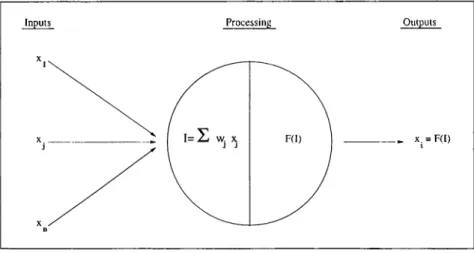
back-propagation neural network. Each node in Figure 2.2 corresponds to a processing unit comparable to a nerve cell in the brain. The first layer is the input layer. The second layer is called hidden layer. There can be more than one hidden layer. The third layer is the output layer. The number of units in each layer is a decision parameter. The connections between the processing units are directed arcs. Each of these arcs has an associated weight. Figure 2.3 represents a detailed unit. This figure illustrates the computation that takes place within each unit. Each unit receives inputs ;r,’s, along the arcs with weight Wj''s, calculates the weighted sum / of these inputs and applies a transfer function F { I ) (activation level). The output of this function, Xi, will be the output of the processing unit. This output is then passed along the arcs connected to this processing unit.

Neural networks are classified based on their learning methods [36] [20] into three categories: supervised learning, unsupervised learning and real time learning. Under the real time learning^ networks continue learning while the network is being used (such as adaptive resoncince theory). For unsupervised

CHAPTER 2. RESEARCH BACKGROUND

12

network is trained by learning a pattern through repecitecl exposure to it and is able to recall the learnt pattern when it solves a categorization or pattern matching problem. For supervised learning, a training data set (containing inputs and their corresponding target output) is used to help the network in arriving at the approjDriate weights. Back Propagation is the best-known supervised learning method with three or more layers. For this algorithm, input is presented to the network and is propagated forward until it reaches the output layer. At the output Iciyer, the output obtciined is compared to the target output corresponding to the given inputs. The error is than propagated backwards along the arcs as to adjust the weights of these circs. The adjustment takes place according to the Delta rule. The experiments carried out in this work cire based on the back propagation algorithm. We consider this algorithm as a black box and we apply it using the NeuralWorks Professional II software

CHAPTER 2. RESEARCH BACKGRO UND

13

Inputs Processing Outputs

x. = F(I)

Figure 2.3: Single processing unit in neural network.

Characteristics of Neural Network

Neural networks hcive been proposed to model systems where the input/output relationship is unknown or too complex; that is to model classes of problems where traditional approaches find it difficult. Therefore, neural networks are not to be used where the already existing approaches perform well since this may result in loss of precision which could be avoided. What distinguishes neural networks from other modeling approaches is their computational speed and learning capabilities as well as their generalization capabilities.

The major distinguishing feature of neural networks is learning the underlying mappings between the input and output variables. Traditionally, when modeling systems, the analyst has to provide some input/output relationship and has to test its validity. Neural networks mark a radically different approach to computing compared to traditional methods. For the case of the Back-propagation neural networks, learning is achieved through adjustment of the weights associated with the interconnections of the networks. In a traditional computer program, every step is specified in advance by the programmer. The network, in contrast, would by itself build the mapping describing the input/output relationship and no programming is required. This is achieved by the learning process. Hence, the neural networks can be used to model highly complex systems. In fact, practitioners welcomed Artificial

CHAPTER 2. RESEARCH BACKGROUND

14

intelligence (A I), including expert systems, since it allowed consideration of qualitative factors and provided a new approach to incorporate intelligence. Neural networks went a step further with respect to AI. Unlike traditional expert systems where knowledge and intelligence is made explicit in the form of rules, neural networks generate their own rules by learning from examples and extending their knowledge. Although the response function is not explicitly formulated as for analytical metarnodels, it is implicitly formulated for the neural network through the architecture applied. These features are likely to give wa}^ to including neui’cil networks in expert systems (ES) and thus enhancing the application of ES in manufacturing or in other decision support systems [36] [28]. Moreover, neural networks can be tested at any time during training. Hence, it is possible to measure a learning curve of the network. In addition, the network Ccui continue learning even after its actual implementation takes place and the training session has finished. As new input/output examples get civailable from the real system, they can be presented to the network to irniDrove its accuracy. Also, if some of the system characteristics (that are not given as input to the network) are changing with time (such as improvement in quality), the network can adjust its weights to these changes thanks to its learning Ccxpabilities.

Another important feature of neural networks is generalization. Although lecirning is based only on limited set of examples, when it comes to applying the neural network model, the network should be able to extend its knowledge to outside this set of examples. The neural network, if properly trained, can provide correct answers when presented with new inputs thcit are different from the inputs in the training set. In order to take full advantage of the above mentioned features of neurcil networks, they must be carefully designed and adjusted to serve the purpose of the study.

Applications of Neural networks in manufacturing environment

Neural networks have a wide range of appliccitions in the manufacturing environments. Zhang and Huang [37] provide a state of the art review of

CHAPTER 2. RESEARCH BACKGROUND 15

the applications of neural networks in general. These applications include:

- group technology[21][14][15], - engineering design,

- monitoring and diagnosis, - process modeling and control, - quality assurance,

- scheduling, and process planning.

Burke and Ignozio review the application of neural networks in OR [4]. Udo and Gupta [10] review the applications of neural networks in manufacturing management systems. The applications reported include (in addition to the one mentioned previously):

- resource allocation and constraint satisfaction, - maintenance and repair,

- datcibase management,

- simulation [30] [

2

- robotics control.

In the survey paper by Udo and Gupta, it appears that the interest in neural networks started mainly since 1987. This corresponds to the same time for which a resurgence of interest was noticed for the use of metamodeling in the manufacturing environments. They also report a list of advantages of neural networks over the conventional computing, such as:

CHAPTER 2. RESEARCH BACKGRO UND

16

- It is trained by example and have the ability to adjust dynamically to changes in the environments.

- It has the ability to generalize from specific examples.

- It has a slow degradation in problems outside the range of the experience. - It has the ability to discover complex rehitionships among inputs

variables, and

- It has speed of response.

Constructing Neural Networks for Simulation Metamodeling

Many design issues are involved in developing a neural network metamodel. Care must be given to these issues as they are essential in developing a reliable and robust neural network metamodel. This is especially important as the metamodels are models of simulations model [.3] [33] [35] [24]. Hence, the error of the network with respect to the real system will be amplified if the network is not ¡properly designed. Whether it is apj^ropriate to use a metamodel or not, is a matter that depends on the application and how much approximation is acceptable. However, it appears that increasingly more people are making use

of metamodels [9]. Figure

2 .1

to selecting the appropriiite variables for the application under consideration and to constructing a valid simulation model, the metamodel itself is a major issue. We have to decide on the internal parameters of the metamodel. Khaw, Lim and Liin [17] report an optimcil design of neural network models based on the Taguchi method in terms of setting the internal parameters of the model for the back propagation-type networks. They claim that their approach improves network reliability and convergence speed. Other authors have selected other approaches. For our experiments, we did not put much emphasis on this part as our aim was not building very precise networks but I'cither examining their behavior.

CHAPTER 2. RESEARCH BACKGROUND

17

significant impact on its performance. The following is a general design

procedure for metamodeling with neural networks. As can be seen, this

procedure does not differ in much from other metamodeling approaches.

• Step

1

measures and mechanisms governing the relationship between inputs and outputs.

• Step 2: Develop a valid simulation model to examine the performance of the system under some experimentcil conditions.

• Step 3: Select the set of variables that will be considered by the network

as inputs. These usually include the decision variables and system

parameters that are expected to be varying during the period of study. Decide on how the performance (or the validity) of the metarnodel will be evaluated.

• Step 4: Decide on how these inputs are to be presented to the network since the input data may need some preprocessing [17].

• Step 5: Decide on the internal design of the neural network. This includes deciding on the number of layers, the number of processing units per layer and the interconnections (full connection, partial connections), etc. [171129].

• Step

6

that takes place in the processing units and the training procedure. There are a number of paradigms available such as back-propagation (widely used in manufacturing applications). Each of these paradigms has several parameters that need to be fine tuned to ensure the appropriate learning and performance of the network.

• Step 7: Once the cvbove issues have been decided upon, training can start. Develop a trciining set using the simulation models and perform

the training. Several iterations may be required between steps 5,

6

CHAPTER. 2. RESEARCH BACKGROUND

18

• Step

8

examples not included in the training set.

Training can continue even after the network has been validated. As new examples from the real system become available, the network can be trained on them; thus further reducing the error with respect to the real system.

In evaluating the precision of the built metamodel, several candidate error measurement methods can be available. It is essential to select an appropriate one. As our experiments have shown, the constructed metamodels may have a different ranking based on the evaluation criterion applied. Therefore, we recommend that a great care should be given to this issue. The importance of this issue is discussed in detail later in the text.

The most widely used implementations of neural networks are software simulators. These simulate the operations of the network on serial computers as these are very much available at low prices. However, the time requirements for developing and implementing the neural networks could be further reduced if hardware with parallel processors are used. Thus, the full potential of neural networks can be further enhanced with developments in hardware.

Drawbacks of Neural Networks

Several shortcomings related to the current applications of neural networks as a metamodeling technique have been reported in the literature [19]. First, constructing a neural network is time consuming as this process requires generating a training set, empirically selecting an appropricite architecture and learning algorithms. Secondly, the accuracy of the network outputs depends on the regularity of the behavior of the system under study (by regularity we mean that the system is subject to the same set of exogenous and uncontrollable factors). This implies that the time horizon of the study must be carefully selected. Thirdly, the validity of the results depends also on the degree of aggregation selected for the input datci. Aggregation ol data is needed in order

CHAPTER 2. RESEARCH BACKGRO UND

19

to reduce the size of the neural network imd the effort required to generate the examples. This would have a negative impact on the precision of the neural network results. The disadvantages mentioned so far are common to most metamodeling techniques.

Another more specific problem related to metamodeling with neural networks is the difficulty to make interpretations and analysis of the input/output relationship. As mentioned previously, the neural network generates its own rules but does not provide them explicitly to the user. In order to get an insight into the input/output relationship, one needs to amrlyze the weights of the connections between the processing unit. This is not an easy task, and it is time consuming. Thus, providing a formal method to analyze the neural network may strengthen its value as a metamodeling approach. Furthermore, the selection procedure for the network architecture, learning algorithm and parameters is in most of the reported cases a trial (empiriccil) process. Some attemi^ts have been made to provide a formal approach to do this task. Khaw, Lim and Lim [17] propose a method based on a Tciguchi approach. Murray [22] used genetic algorithms to perform this tcisk. Further dehciencies in the literature are concerned with the lack of development of learning algorithms. Research in this direction may allow more exploration of the full potential of neural networks.

2.4

Neural networks as a simulation meta­

modeling approach

Our research is focused on simulation metarnodeling with neural networks for the purpose of estimating system performance measures. Zhang and Huang [37] have reported cin increasing interest of the use of neural networks in the

manufacturing environment since 1987. Starting the same period, Yu and

Poplewell [35] report an increasing interest in simulation metamodeling. This illustrates that these two different techniques have an increasing potential of contribution to improving the management of manufacturing systems. Despite

CHAPTER 2. RESEARCH BACKGRO UND 2 0

this interest, efforts to combine metamodeling and neural networks through the use of neural networks as a simulation metamodeling approach has not been much. In fact, for this type of applications of neural networks, the related literature is not abundant. Seven papers applying the back propagation neural networks as a simulation metamodel for the management of manufacturing systems are surveyed.

Chryssolouris et ah [

6

computational efforts required in the long trial process that is associated with using simulation alone for the design of a manufacturing system. The simulation model is used to generate the performances (4 performances

measures are recorded) of the system under different designs. The neural

networks is then used in an inverse manner. The input of the neural network is the desired levels of the performances of the system cind the output would be the design that would achieve those levels of performance. Although this cipplication was successful, some questions were raised regarding the complexity of the system and regarding the complexity of the application itself. In fact, because of the small size of the system considered, the number of design alternatives is not large. However this application, indiccites a potential use of neural networks as system design has an important impact on its performance and often the design phase is time consuming because of the large number of alternatives.

Simulation metamodeling with neural networks mostly is applied as a tool for determining operational policies since it is in this type of applications that time is more crucial. Chryssolouris has developed a task assignment procedure that is based on multi-criteria, called MADEMA (MAnufacturing DEcision MAking). This approach combines the system performance criteria according to some given weights. Chryssolouris et ah [5] used a neural network metamodel to determine the weights required to achieve some given levels of the multiple criteria. Although the application showed some good results and a good ability of neural networks to handle complex rehitions, one may question the effect of the small range of the inputs and the effect of system complexity. Hurrion [13] used a neural network to estimate confidence intervals

CHAPTER 2. RESEARCH BACKGROUND 21

for the performance of an inventory depot. This application revealed that neural networks were equally successful to estimate mean performcince as well as their corresponding confidence intervals. Moreover, this work highlighted the capabilities of neural networks to model problems with large range of inputs and complex input/output relation but still does not provide an insight on the effect of system complexity nor on the effect of stochasticity. Another case was examined by Pierreval [27] to investigate the ability of neural networks to estimate mean machine utilization of a deterministic small sized problem. The results were encouraging as in this problem input range was wide and also the neural networks showed its ability to learn and generalize properly. The questions that raises here may be regarding the effect the performance measure, stochasticity and system complexity. Pierreval [29] later proposed a neural network architecture to be used for ranking the performance of dispatching rules on a stochastic flow shop type system. Neural networks have performed well and highlight the modeling flexibility that modeling with neural networks can offer. Here one may question the effect of system configuration (flow shop vs. job shop). The work reiDorted by Philipoom et al. [26] gives some other type of application of neural networks as a simulation metamodel. Neural networks are applied to assign due dates for jobs bcised on system characteristics and system status when jobs enter system. The use of neural network for individual jobs contrasts with the use of neural networks to get aggregcite system measures

(such as mean flow time in the ¡previously rneirtioned publications). The

performance of neural metamodels compared favorably with regression based metamodels and showed another interesting type of application. Kilmer et al. [18] report a possible use of neural metamodel for a service activity, an emergency department. They tested the validity of metamodel, with respect to the real system, and it appears that the validity is high.

In the seven publications reported in the last 2 paragraphs, the constructed neural network metamodels achieved reasonably good results. The authors showed that neural networks are a very promising tool for predicting system measures. However, these case studies deal with systems of reduced complexities or of deterministic nature and do not allow us to generalize on

CHAPTER 2. RESEARCH BACKGROUND 2 2

the estimating capabilities of neural networks. The following set of questions summarizes some of the future research issues that still need to be investigated:

- How to assess neural metamodel performance?

- What is the effect of system size on the performcince of the neural network?

- To what extent can the neural network handle system stochasticity? - Do stochastic factors effect differently network performance?

- Is the metamodel performance affected by the fact that the system is in transient state or in steady state?

- Is the performance of the rnetamodel affected by the level of cictivity of the system?

- What is the effect of the performance measure being predicted?

- What is the effect of the network configuration (size, number of layers, learning ixite ...) on the performance of the network?

- Does system configuration (flow shop-job shop) have an effect on the performance the developed neural networks?

- How robust is the neural metamodel to noisy data, to delta outside the training range?

- How adaptive is it to gradual snicill changes in the system over time (such as gradual improvements in quality)?

- What are the conqDutational requirements in terms of computer time? - How to select the size of training and test data?

CHAPTER 2. RESEARCH BACKGRO UND

23

This small set of questions is representative of the current vacancies in the literature. In this work, we don’t attempt to answer all these questions. Rather we concentrate only on the first eight questions. We don’t intend to give extensive and final answers to these questions. We aim at constructing

experiments that would allow us to get an insight on these issues. As a

matter of fact, our work investigates two types of application of neural network metamodels: estimating long term system performance and short term system performance.

For the first application, we will investigate the effect of:

* Performance measure: Mean machine utilization and mean job tardiness. * System complexity: Simple vs. complex system.

* Stochasticity: deterministic, stochastic interarrival times only, stochastic processing times only or both stochcistic.

* Demand on system: low, medium and high. * Metamodel error assessment criteria.

In all the reports we described previously, neural metamodels cire examined in terms of estiniciting long term performance, and the civailable literature is not abundant yet. For estimating short term performance, we could not find any reports on the use of neural metcimodels for such applications. For this we also examine such an application in order to gain insight on the effect of this issue and so we can get an idea about the possible use of neural metamodels for real time decision support. With the second application, we will consider the mean job tardiness as a system performance measure and we allow the system to be deterministic or to be subject to stochastic processing times and interarrival times. That is, we investigate the effect of:

* Initial system status.

CHAPTER 2. RESEARCH BACKGROUND

24

* Metamoclel error assessment criteria.

For both aj^plications, we preview the effect of clue date tightness factor and of the effect of the size of training set. In order to preserve a basis of comparison, we use the same system structure, neural network architecture and same error assessment criteria. The neurcil network learning algorithm is considered as a black box and we don’t attempt to improve it. We also

do not C c ir r y out extensive fine tuning of the parameters because it is time

demanding and because our emphasis is more on developing an understanding of the behavior of neural metaniodels with respect to the factors previously mentioned. The next 2 chapters investigate long term mean machine utilization and mean job tardiness respectively. The fifth chapter examines the situation for the short term mean job tardiness. Finally, we give our conclusions and future research directions in the last chapters.

Chapter 3

Estimating Long Term Machine

Utilization

In this chapter, we investigate the capabilities of neural metamoclel in estimating mean machine utilization as a system performance measure. We consider two job shop systems, which we would refer to as case one cind case two. The first job shop system is a simple one with four machines and three distinct product types. The second system is a comple.x one. This system can be considered as an extension of the first system, to include more machines

and more product types. This extension is made in such a Wciy as to keep

a basis of comparison between the two cases. This is achieved by adding three more machines and three more job types to the first system. While the job types common to both systems keep the same parameters in terms of processing and routing requirements, the new product types have processing requirement on both the old and the new machines. Hence, the first system is a subset of the second one. This allows us to investigate the effect of increased system complexity by studying the second system and comparing it to the first one. Therefore, the term “system complexity” in this study would refer to increased system size (increased number of machines and increased number of job types) as well as increcised interactions between the different components of the system. For each of the two cases, we describe the experimental settings

through describing the system, the simulation models, the neural network metamodels cind the error assessment approaches. The next section lays down the results and discussions. The last section of the chapter compares the two Ccises.

3.1

Case 1: Simple System

In this first case, we consider the work reported by Pierreval [27] as the

starting point. His work tries to estimate mean machine utilization for a

deterministic system. In the first step, we .simply repeat this work. In our experiments, however, the back propagation learning algorithm is improved by adding a momentum term. The second step is to investigate the stochastic configurcitions of the same system (stochastic arrived times only, stochastic processing times only or both) and to test the robustness of the metamodels designed for the deterministic configuration to inputs that lie outside the training range.

3.1.1

Experimental settings

System description

CHAPTER 3. ESTIMATING LONG TERM MACHINE UTILIZATION

26

This study is based on the work done by Pierreval [27]. His experiment consists of running a simulation model for a deterministic job shop system. Based on this model, a neural network metamodel to estimate machine utilization is constructed. This job shop system, he used, is deterministic. It is composed of four machines and three free transporters. Three job types are entering the

system. Jobs arrive independently to the .system at constant rates: Ai, A

2

A

3

discipline (f). The waiting discipline, could be either Shortest Processing

In this first case, we consider four possible configurcitions of this job shop system; a deterministic configuration, a configuration with stochastic interarrival times only, a configuration with stochastic processing time only and fiiicilly a configuration with stochastic interarrival times and processing times. Our work is based on the same system. All the relevant data can be obtained from the sample codes provided in Appendix C. For the case of stochastic arrivcil times, those same values of the constant interarrival

times Ai, A

2

3

distributions. Similarly, the constant values of the processing times, used in the deterministic configuration, are used as means of the corresponding exponential distributions in the stochastic processing times configuration. The choice of the exponential distribution for both factors (cirrival and processing times) appears reasonable since a large number of the reported simulation experiments use this

distribution which seems to match real life as well [

1

Simulation Models

CHAPTER 3. ESTIMATING LONG TERM MACHINE UTILIZATION

27

The simulation models of the system described above are developed and used

to run the job shop system for various configurations. The production is

performed in two shifts. For the deterministic configuration, the model is run during one week of work (5 days), plus one day of transient phase. For the

stochcistic case, a transient period of

2

run for 15 days, to form 5 batches of three days each (Batch means approach is used through out this study). We are interested in finding the average

machine utilizations ¡.ii, H2, ¡.iz and

/¿4

bottleneck machines as well cis under-utilized machines. Therefore, given cin

input combination of Ai, A

2

3

model to record the output combination //

2

/¿3

/¿4

outputs are the true values of these variables that the neural metamodel has to estimate. The combinations of these inputs and outputs would compose one example in the data set that is presented to the neural networks either in a training set or as a test set. The simulation models are developed in SIM AN language [25]. Sample model and experimental frames are provided

CHAPTER 3. ESTIMATING LONG TERM MACHINE UTILIZATION

28

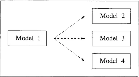
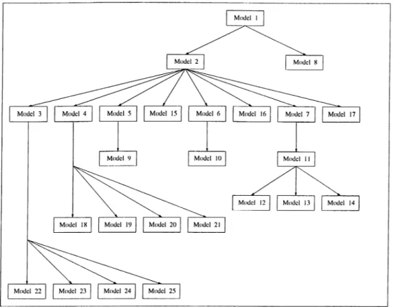
in ApjDendix C. Four simulation models are used; each corresponding to one of the configurations mentioned above. Table .3.1.1 in Appendix B shows the list of the models built. Figure 3.1.1 illustrates the relationship between those models. For each model the corresponding training iind test sets are generated. In terms of machine utilization, the characteristics of the data sets generated from these models are quite identical for all the models examined in the first case, and are as follows:

- minimum utilization: 14..5% - mean utilization: 45.2%

- standard deviation of utilization: 17.7%

- maximum utilization:

1 0 0

Model 2

Model 1

_{Model 3}

Model 4

Figure 3.1: Mean Utilization: Simple System: Relationship between models.

This means that independently of any factor being stochastic or determin­ istic, the resulting sets are similar. This may lead us to think that similar results can be obtained from all the models.

For model

1

and is similar to test Set #

1

generate Set

^ 6

from [100,120]. Test sets ^ 5 and

# 6

metamodel with respect to inputs thcit lie outside the range of the training data and hence allow evaluating generalization capabilities of neural metcimodels. Two sets are used in order to see how the performance of the neural metamodel evolves as we move far from the range of the inputs of the training set.

As each data set (training or test sets) require a set of examples, we need to create the set of inputs to be given to the simulation model in order to generate the true values of the variables of interest (mean machine utilizations), and to be presented to the neural network in order to generate estimates of the variables of interest. A SIMAN code wcis used to randomly generate the values of the inputs in the desired range from a uniform distribution. Another

ap

2

techniques. However, the first api^roach was used because it corresponds to real life more where examples would follow a random scheme. Appendix C shows the model and experimental frames for this input data generator model.

Neural Network Metamodels

CHAPTER 3. ESTIMATING LONG TERM MACHINE UTILIZATION

29

Several Back-propcigation neural networks are designed with various architec­ tures (number of iDrocessing units and layers) and various combinations of network parameters (learning rate, momentum term). No bias is introduced, nor dynamic adjustment of the learning parameters are used. The sigmoid function is used as the transfer function in the processing units. Inputs are

scaled in the interval [0,1]. Table

3

1 .2

of the networks constructed for each model. In this Table, the name assigned to each neural network are as follows; Expl_A_B. This coding should be read as the name of the neural network number B developed as a metamodel for model A of this first .set of experiments. An example would be; Expl_2_3. This describes the network number 3 designed for model 2 of this first set of experiments. Refer to the generic circhitecture given in Figure 2.1.