On the numerical solution of Kronecker-based infinite level-dependent QBD processes

(1)

Contents lists available atScienceDirect

Performance Evaluation

journal homepage:www.elsevier.com/locate/peva

On the numerical solution of Kronecker-based infinite

level-dependent QBD processes

H. Baumann

a

,

T. Dayar

b,∗

,

M.C. Orhan

b

,

W. Sandmann

c

a_{Department of Applied Stochastics and Operations Research, Clausthal University of Technology, D-38678 Clausthal–Zellerfeld,} Germany

b_{Department of Computer Engineering, Bilkent University, TR-06800 Bilkent, Ankara, Turkey} c_{Campus E1 3, Room 325, Saarland University, D-66123 Saarbrücken, Germany}

a r t i c l e i n f o

Article history:

Available online 11 June 2013 Keywords:

Markov chain

Level-dependent QBD process Kronecker product

Matrix analytic method Steady-state expectation Call center

a b s t r a c t

Infinite level-dependent quasi-birth-and-death (LDQBD) processes can be used to model Markovian systems with countably infinite multidimensional state spaces. Recently it has been shown that sums of Kronecker products can be used to represent the nonzero blocks of the transition rate matrix underlying an LDQBD process for models from stochastic chemical kinetics. This paper extends the form of the transition rates used recently so that a larger class of models including those of call centers can be analyzed for their steady-state. The challenge in the matrix analytic solution then is to compute conditional expected sojourn time matrices of the LDQBD model under low memory and time requirements after truncating its countably infinite state space judiciously. Results of numerical experiments are presented using a Kronecker-based matrix-analytic solution on models with two or more countably infinite dimensions and rules of thumb regarding better implementations are derived. In doing this, a more recent approach that reduces memory requirements further by enabling the computation of steady-state expectations without having to obtain the steady-state distribution is also considered.

1. Introduction

Continuous-time infinite level-dependent quasi-birth-and-death (LDQBD) processes [1–3] are continuous-time Markov chain (CTMC) processes that have block tridiagonal transition rate matrices of the form

Q

=







Q0,0 Q0,1 Q1,0 Q1,1 Q1,2

... ... ...

Ql,l−1 Ql,l Ql,l+1

... ... ...







when their states are appropriately ordered. This study is about their numerical steady-state analyses, and hereafter, we shall be omitting the terms continuous-time and infinite in designating the LDQBD models we consider since they are all continuous-time and infinite.

∗_{Corresponding author. Tel.: +90 312 290 1981; fax: +90 312 266 4047.}

E-mail addresses:hendrik.baumann@tu-clausthal.de(H. Baumann),tugrul@cs.bilkent.edu.tr(T. Dayar),morhan@cs.bilkent.edu.tr(M.C. Orhan),

sandmann@cs.uni-saarland.de(W. Sandmann).

(2)

In the following, all vectors are column vectors as in linear algebra, except state vectors, consistent with the conventional definition of state probability vectors as row vectors. e represents a column vector of 1’s. eirepresents the ith column of the identity matrix. diag

(

a

)

denotes a diagonal matrix with the entries of vector a along its diagonal. The lengths of the vectors are determined by the context in which they are used,Tdenotes transposition,

×

when used with sets denotes Cartesian product,

⊗

denotes Kronecker product [4],

1

denotes the indicator function, Z and R stand respectively for the sets of integers and real numbers, whereas Z+and R≥0denote their nonnegative subsets.

Now, letSdenote the irreducible state space of the LDQBD process under consideration, the state of the LDQBD process at time t be given by X

(

t

) = (

X1

(

t

), . . . ,

Xn

(

t

)) ∈

S, and

{

X

(

t

) ∈

S

,

t

≥

0

}

be the associated n-dimensional CTMC process. Furthermore, let the probability of the LDQBD process being in state x

=

(

x1

, . . . ,

xn

) ∈

Sat time t be expressed as

Pr

{

X

(

t

) =

x

} =

Pr

{

X1

(

t

) =

x1

, . . . ,

Xn

(

t

) =

xn

}

. Levels define a partition ofS; that is,S

=



∞

l=0S(

l)_and_S(l)

_∩

_S(m)

_{= ∅}

_{for l}

_̸=

_{m and l}

_,

_m

_∈

Z+, whereS(l)is the subset

of states corresponding to level l. Therefore, the nonzero blocks at level l satisfy

Ql,l−1

∈

R|S (l)_|×|_S(l−1)_| ≥0

,

Ql,l

∈

R|S (l)_|×|_S(l)_|

,

Ql,l+1

∈

R|S (l)_|×|_S(l+1)_| ≥0

with the exception that there are only two boundary blocks at level 0.

We consider ergodic LDQBD processes and investigate the numerical computation [5,6] of their steady-state probability measures. The steady-state probability distribution row vector of an ergodic LDQBD process is defined as

π =

limt→∞Pr

{

X

(

t

)}

, and it satisfies

π

Q

=

0

,



x∈S

π(

x

) =

1

.

In particular, the steady-state vector of an ergodic LDQBD process can be accordingly partitioned and expressed as

π = (π

(0)

_{, π}

(1)

_{, . . .),}

and its subvector at level

(

l

+

1

)

can be obtained from the matrix analytic equation

π

(l+1)

₌

_π

(l)_R l

as shown in [1], once the conditional expected sojourn time matrix at level l

Rl

=

Ql,l+1

(−

Ql+1,l+1

−

Rl+1Ql+2,l+1

)

−1

is determined for l

∈

_Z+. Note that

π

(l)

∈

R1×|S

(l)_| ≥0 ,

π

( l+1)

_∈

R1×|S (l+1)_| ≥0 , and Rl

∈

R|S (l)_|×|_S(l+1)_| ≥0 . LDQBD processes are a

generalization of QBD processes originally proposed in [7,8] and improved over the years [2,9] with two quadratically con-vergent algorithms for their steady-state analyses. These algorithms are logarithmic reduction [10] and cyclic reduction [11]. In the level dependent context, the situation is more complicated since the conditional expected sojourn time matrix is not constant and changes from level to level.

In many cases, the ergodicity of an LDQBD process can be established by relatively easy to check conditions on the 1-dimensional CTMC defined over its levels [12]. For computational purposes however, it is preferable to consider Lyapunov function methods as discussed in [13,14], so that lower and higher level numbers (called Low and High, respectively) can be computed as in [15–17] between which a specified percentage of the steady-state probability mass lies when the LDQBD is ergodic. It is the latter approach we follow here. In this way, steady-state measures can be computed exactly up to machine precision by choosing

(

High–Low

)

sufficiently large as discussed in [17].

Systems of stochastic chemical kinetics [18–21] and queueing networks [2,5,22–24] are two classes of problems that can be modeled as LDQBD processes using the described n-dimensional state representation with some countably infinite variables. For the former class of problems, countably infinite variables represent numbers of molecules of each chemical species existing in the system. The remaining variables, if any, are finite. Up until recently, stochastic simulation [25,26] seemed to be the only viable approach that would yield relatively accurate results for this class of problems. However, it has been shown in [17] that systems of stochastic chemical kinetics can be modeled as LDQBD processes with the level number determined by the maximum value among the countably infinite variables. Inspired by hierarchical Markovian models (HMMs) introduced in [22], the result in [17] has been taken one step further in [16] by providing a Kronecker-based representation for the nonzero blocks Ql,l−1

,

Ql,l

,

Ql,l+1at each level to cope with the multidimensionality of the product state

space of variables and its reachability. As suggested in [27] and as observed to be the best overall choice in [17], again RHighis set to 0 to initiate the computational procedure associated with the matrices of conditional expected sojourn times. Therein, a comparative study between stochastic simulation and the matrix analytic approach has also been undertaken. Naturally, the matrix analytic approach yields an accuracy measure obtained by computing the residual norm of the solution which is not possible with simulation.

It is the latter class of problems on which we concentrate in this paper by considering various queueing network models of call centers with multiple types of customers. In this context, the countably infinite variables represent occupancies of queues with unbounded waiting space and finite variables represent occupancies of server pools. The interplay between finite variables and countably infinite variables in these models is more intricate than that of models of stochastic chemical kinetics systems. This requires us to extend the form of the transition rates used in [16]. To that end, we resort to generalized

(3)

functional transitions of stochastic automata networks (SANs) [28–30], and let the form of the dependency of the transition rate on the values of the variables be more general. As we shall see, the use of such transition rates does not pose a computational efficiency problem, since a direct method in which each nonzero block is processed once is employed in the matrix analytic solution. In other words, each function is evaluated once for each state in the truncated state space



High

l=LowS(l)during analysis. An implication of this extension is that not only do we need to compute partitions of state spaces of countably infinite variables as in [16], but now we also need to compute subpartitions of these partitions and partitions of state spaces of finite variables to obtain a Kronecker-based representation for the nonzero blocks of Q .

We also consider the more recent approach in [31] that reduces memory requirements further by enabling the computation of steady-state expectations without having to obtain the steady-state distribution. The approach is inspired by a Horner-like computational scheme in which only the conditional expected sojourn time matrix at level l needs to be allocated in step l; otherwise, there are no time savings. In other words, not all Rlmatrices need to be stored simultaneously. With this memory efficient approach, a tandem queueing network of two single server queues with infinite waiting spaces and customers departing from the first queue leaving the system with a probability depending on the length of the second queue is analyzed. The steady-state measures computed are those that are based on average costs or rewards, moments, and cumulants. However, there is one drawback; it is the loss of the accuracy measure because the steady-state distribution is no longer available. Ongoing work is concerned with obtaining accuracy measures for this approach as well, but they are not yet available.

Taking into account the experience gained from the Matlab implementation used in [16], we provide an implementation in C based on the Nsolve package of the Abstract Petri Net Notation (APNN) Toolbox [32]. Our objective in doing so is to have more control over memory usage and timings. Since the number of states within each level increases with increasing level number in the models we consider, we conduct numerical experiments with timing results to see how and when memory should be allocated and deallocated, and whether the conditional sojourn time matrices should be stored as full or sparse matrices. With the existing continuous improvement in computer technology, we believe we have reason to invest in numerical analysis approaches for multidimensional Markovian models as those discussed here to obtain more accurate results at a finer level of detail.

In the next section, we extend the specification for the class of models considered to build a Kronecker representation of the nonzero blocks in Q and introduce a running example. Due to space limitations, we refrain from discussing the models of stochastic chemical kinetics systems used before and refer to [33]. We also introduce two other models of call centers at the end of Section2. In Section3, we discuss implementation issues including the choice of Lyapunov functions and provide results regarding memory usage for different implementations after giving the algorithm for the computation of the steady-state distribution of LDQBD processes. In Section4, we report on the results of numerical experiments with the matrix analytic approach on the models introduced earlier to identify better implementations. In Section5, we conclude. 2. Kronecker representation

We consider Markovian systems with interacting subsystems. The state spaceSis irreducible, countably infinite, and

n-dimensional with nIcountably infinite state variables and nFfinite state variables, where nI

≥

2

,

nF

≥

0, and n

=

nI

+

nF. Hereafter, we shall be omitting the word ‘state’ and referring to state variables as variables. The state space of variable xh is denoted byShandSh

⊆

Z+for h

=

1

, . . . ,

n. Without loss of generality, we assume that the first nIindices correspond to countably infinite variables. Hence,Shis countably infinite for h

=

1

, . . . ,

nIand finite for h

=

nI

+

1

, . . . ,

n. Clearly, not all states in the product state space

×

n

h=1Share necessarily reachable. However, each state inSis reachable from every other state inSdue to our assumption of irreducibility. In many cases,Sis a proper subset of the product state space (i.e.,

S

⊂ ×

n_h₌₁Sh). Indeed, it is as such in the models of call centers introduced in the next section.

The n-dimensional Markovian models we consider are defined by a set of K transition classes over S and x

=

(

x1

, . . . ,

xn

) ∈

Z+1×ndenotes a state inS. We relax some of the assumptions made in [16] so as to be able to analyze a larger

class of models. Observe in particular that we do not require product form transition rates here (cf. Definition 1 in [16]). Definition 1. The kth transition class is a pair (

α

k

, v

(k)), where

α

k

∈

R≥0and

v

(k)

∈

Z1×nare respectively its transition rate and state change vector for k

=

1

, . . . ,

K . The first element of the pair,

α

k

(

x

)

, is a function of state x

∈

Sand specifies the transition rate from state x to state

(

x

+

v

(k)

_{) ∈}

_S_{. The second element of the pair,}

_v

(k)_{, specifies the successor state of the} transition, where

v

_h(k)denotes the value change in variable xh

∈

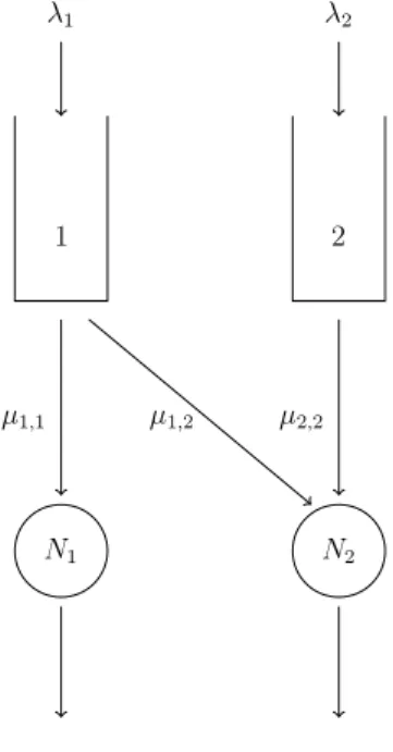
Shdue to the kth transition class.

Example 1 (N-Model). Consider the parallel service system inFig. 1known as the N-model under the threshold routing control policy proposed in [34]. In this model, there are two types of customers, two types of infinite queues, and two types of server pools. Customers of type 1 can be in queue 1, server pool 1, or server pool 2, but type 2 customers can only be in queue 2 or server pool 2. Hence, x

=

(

x1

,

x2

,

x3

,

x4

,

x5

)

is a possible state representation, where x1

,

x3, and x4denote the

number of type 1 customers in queue 1, pool 1, and pool 2, respectively, whereas, x2and x5denote the number of type 2

customers in queue 2 and pool 2, respectively. Then, n

=

5

,

nI

=

2, and nF

=

3. Type i customers arrive to the system according to a Poisson process with rate

λ

iand server pool i has Niservers with exponentially distributed service times for

(4)

Fig. 1. N-model.

Table 1

Transition classes of the N-model.

k αk(x) v(k) 1 λ11x3=N11x4+x5=N2 e T 1 2 λ11x3=N11x4+x5<N2 e T 4 3 λ11x3<N1 e T 3 4 λ21x4+x5=N2 e T 2 5 λ21x4+x5<N2 e T 5 6 µ1,1x31x1=0 −eT3 7 µ1,1x31x1>0 −eT1 8 µ1,2x41x1=01x2=0 −e T 4 9 µ2,2x51x1=01x2=0 −eT5 10 µ1,2x41x1>01x2=0 −e T 1 11 µ2,2x51x1>01x2=0 (−e1+e4−e5)T 12 µ1,2x41x1≤M1x2>0 (−e2−e4+e5)T 13 µ2,2x51x1≤M1x2>0 −e T 2 14 µ1,2x41x1>M1x2>0 −eT1 15 µ2,2x51x1>M1x2>0 (−e1+e4−e5) T

if it has idle servers (i.e., x3

<

N1) and receives service at a rate of

µ

1,1. If there are no idle servers in pool 1 (i.e., x3

=

N1), an

arriving type 1 customer joins pool 2 if it has idle servers (i.e., x4

+

x5

<

µ

1,2. If there are

no idle servers in either pool (i.e., x3

=

N1, x4

+

x5

=

N2), an arriving type 1 customer enters queue 1. On the other hand, an

arriving type 2 customer joins pool 2 if it has idle servers (i.e., x4

+

x5

<

µ

2,2; otherwise

(i.e., x4

+

x5

=

N2) it enters queue 2. Upon departure of a customer from server pool 2, the first customer in queue 1 joins

it if the number of type 1 customers in queue 1 exceeds a given threshold M (i.e., x1

>

M); otherwise (i.e., x1

≤

M) the first

customer in queue 2 joins it. Hence, type 1 customers take nonpreemptive priority over type 2 customers in server pool 2 when the number of type 1 customers in queue 1 exceeds M.

The transition classes of this model are given inTable 1. Note that the number of transition classes is K

=

15

,

N1and N2

are positive integers, M

∈

_Z+, and

λ

1

, λ

2

, µ

1,1,

µ

1,2

, µ

2,2

∈

R>0.

The following definition associates transition matrices with each transition class inDefinition 1. Being motivated by generalized functional transitions in SANs [28–30], we let the form of the dependency of the transition rate on the values of the variables be more general. In order to achieve this, the local state dependent transition rates are moved out of the transition matrices and replaced with 1’s in their respective places (cf. Definition 2 in [16]). As we shall see, the use of such transition rates, which are functions of (global) state x

∈

Srather than product of functions of local states xh

∈

Sh for h

=

1

, . . . ,

n, does not pose a computational efficiency problem in this context, since a direct method in which each

(5)

nonzero block is processed once is employed in the matrix analytic solution. In other words, each function is evaluated once for each global state in the truncated state space



High

l=LowS(l)during analysis. Note that, here we do not differentiate between countably infinite variables and finite variables in defining the transition matrices (cf. Definition 2 in [16]).

Definition 2. The transition matrix of variable x_h

∈

_S_hfor the kth transition class, denoted by Z(k,h)

∈

_R|Sh|×|Sh| ≥0 , for

h

=

1

, . . . ,

n and k

=

1

, . . . ,

K is given entrywise as Z(k,h)

(

xh

,

yh

) =



1 if yh

=

xh

+

v

h(k)

0 otherwise for xh

,

yh

∈

Sh

.

Here we refrain from providing transition matrices of models in Kronecker form due to the space limitations and because they all follow in a straightforward manner fromDefinition 2and the respective transition classes as was shown in [16]. Our goal is to obtain a Kronecker representation for the nonzero blocks of Q from the transition rates and the transition matrices ofDefinitions 1and2, respectively. To this end, we use the same level definition in [16] since the maximum valued countably infinite variable xh

∈

Shfor h

=

1

, . . . ,

nIin any state x

∈

Schanges by at most one through any transition due to the particular form of the state change vectors

v

(k)_{in the transition classes of models we consider.}

Definition 3. The subset of states corresponding to level l

∈

_Z+is given by S(l)

= {

x

∈

S

|

l

=

max

(

x1

, . . . ,

xnI

)},

so thatS

=



∞ l=0S(l).

Note that the set operation underlying the Kronecker product is the Cartesian product, and therefore the subset of states at each level needs to be expressed as a union of Cartesian products of state space partitions of the countably infinite variables. Hence, level definitions, such as l

=



nI

h=1xh, which have arithmetic dependencies among countably infinite variables seem to be less suitable in trying to come up with a Kronecker representation.

For each level l, the values a variable can take depend on the values of other variables. Therefore, as in [16] first we define the partitions of state spaces of countably infinite variables where there is no such dependency in a way similar to HMMs in [22]. Then we introduce a partition ofS(l)inDefinition 3based on the partitions of state spaces of countably infinite variables. Definition 4. Let S_h(l,u)

=



_{

_x h

|

0

≤

xh

≤

l

−

1

}

if h

<

u

{

l

}

if h

=

u

{

xh

|

0

≤

xh

≤

l

}

if h

>

u for h

,

u

=

1

, . . . ,

nI

,

andSh(l,u)

=

Shfor h

=

nI

+

1

, . . . ,

n, and u

=

1

, . . . ,

nI. Then the uth partition ofS(l), denoted byS(l,u), for u

=

1

, . . . ,

nI satisfies

S(l,u)

= {

x

∈

_S(l)

|

(

x₁

, . . . ,

x_n

) ∈ ×

n_h₌₁Sh(l,u)

}

,

so thatS(l)

=



nI

u=1S(

l,u)_{. Without loss of generality, the partitions}_S(l,u)_{are assumed to be ordered within}_S(l)_{according to}

increasing partition index, u.

Example 1 (N-Model (cntd.)). The partitions ofS(_hl)for h

=

1

, . . . ,

n and l

≥

0 are computed fromDefinition 4as

S₁(0,1)

=

S₂(0,1)

= {

0

}

,

S₃(0,1)

= {

0

, . . . ,

N1

}

,

S4(0,1)

=

S (0,1) 5

= {

0

, . . . ,

N2

}

,

S₁(l,1)

= {

l

}

,

S₂(l,1)

= {

0

, . . . ,

l

}

,

S₃(l,1)

= {

0

, . . . ,

N1

}

,

S₄(l,1)

=

S₅(l,1)

= {

0

, . . . ,

N2

}

,

S₁(l,2)

= {

0

, . . . ,

l

−

1

}

,

S₂(l,2)

= {

l

}

,

S₃(l,2)

= {

0

, . . . ,

N1

}

,

S₄(l,2)

=

S₅(l,2)

= {

0

, . . . ,

N2

}

for l

>

0

.

Note that partitionS(l,u)_{consists only of reachable states, and is a subset of the Cartesian product of state space partitions} of all variables since certain values of finite variables may yield unreachable states (cf. Definition 5 in [16]). Therefore, we define partitions ofS(l,u)_and_S(l,u)

h inDefinition 4to eliminate any unreachable states due to finite variables. Definition 5. The ith partition ofS(l,u), denoted byS(l,u,i), for i

=

1

, . . . ,

I(l,u)is given by

S(l,u,i)

= {

x

∈

S(l,u)

|

(

x1

, . . . ,

xn

) ∈ ×

nh=1S (l,u,ih) h

}

,

so thatS(l,u)

₌



I(l,u) i=1 S(l,u,i), whereS (l,u,ih)

h is the ihth partition ofSh(l,u)for h

=

1

, . . . ,

n

,

u

=

1

, . . . ,

nI, and ih

=

1

, . . . ,

Ih(l,u). Without loss of generality, the partitionsS(l,u,i)_{are assumed to be ordered within}_S(l,u)_{lexicographically according to the} corresponding partition indices,

(

i1

, . . . ,

in

)

.

(6)

Note that, partitionS(l,u,i)consists only of reachable states, and is a subset of the Cartesian product of the state space subpartitions of all variables since certain values of finite variables may yield unreachable states. As we shall see, the values of I(l,u)_{and I}(l,u)

h for h

=

1

, . . . ,

n depend on the model, and although I(l,u)

=



n

h=1I (l,u)

h was true for all the models considered in [16] (due to the fact that I(l,u)_{and I}(l,u)

h for h

=

1

, . . . ,

n were all 1’s), it need not be true in general.

Example 1 (N-Model (cntd.)). The total number of type 1 and type 2 customers cannot exceed the number of servers in pool 2, so x4

+

x5

≤

N2. Besides, a queue can be nonempty only if all servers capable of serving that queue are busy. Then, x3

=

N1

if x1

>

0, and x4

+

x5

=

N2if x1

>

0 or x2

>

0. Due to these dependencies, partitions ofS(h0,1)for h

=

1

, . . . ,

n andS(0,1) can be written fromDefinition 5as

I₁(0,1)

=

I₂(0,1)

=

I₃(0,1)

=

1

,

I₄(0,1)

=

I₅(0,1)

=

N2

+

1

,

S1(0,1,1)

=

S( 0,1,1) 2

= {

0

}

,

S( 0,1,1) 3

= {

0

, . . . ,

N1

}

,

S4(0,1,i)

= {

i

−

1

}

,

S( 0,1,i) 5

= {

N2

+

1

−

i

}

for i

=

1

, . . . ,

N2

+

1

,

so that I(0,1)

₌

₍

_N 2

+

1

)(

N2

+

2

)/

2 and S(0,1,i)

= {

0

} × {

0

} × {

0

, . . . ,

N1

} × {

x4

} × {

x5

}

,

where i

=



x4 j=1

(

N2

+

2

−

j

) +

x5

+

1 for x5

=

0

, . . . ,

N2

−

x4and x4

=

0

, . . . ,

N2.

Partitions ofS(_hl,1)for h

=

1

, . . . ,

n andS(l,1)and l

>

0 can be written fromDefinition 5as

I₁(l,1)

=

I₂(l,1)

=

1

,

I₃(l,1)

=

2

,

I₄(l,1)

=

I₅(l,1)

=

N2

+

1

,

S₁(l,1,1)

= {

l

}

,

S(₂l,1,1)

= {

0

, . . . ,

l

}

,

S₃(l,1,1)

= {

0

, . . . ,

N1

−

1

}

,

S3(l,1,2)

= {

N1

}

,

S₄(l,1,i)

= {

i

−

1

}

,

S₅(l,1,i)

= {

N2

+

1

−

i

}

for i

=

1

, . . . ,

N2

+

1

,

so that I(l,1)

₌

_N 2

+

1 and S(l,1,i)

= {

l

} × {

0

, . . . ,

l

} × {

N1

} × {

x4

} × {

x5

}

,

where i

=

x4

+

1 and x5

=

N2

−

x4for x4

=

0

, . . . ,

N2.

Partitions ofS(_h1,2)for h

=

1

, . . . ,

n andS(1,2)_{can be written from}_{Definition 5}_as

I₁(1,2)

=

I₂(1,2)

=

1

,

I₃(1,2)

=

1

,

I₄(1,2)

=

I₅(1,2)

=

N2

+

1

,

S₁(1,2,1)

= {

0

}

,

S₂(1,2,1)

= {

1

}

,

S₃(1,2,1)

= {

0

, . . . ,

N1

}

,

S₄(1,2,i)

= {

i

−

1

}

,

S₅(1,2,i)

= {

N2

+

1

−

i

}

for i

=

1

, . . . ,

N2

+

1

,

so that I(1,2)

=

N2

+

1 and

S(1,2,i)

= {

0

} × {

1

} × {

0

, . . . ,

N1

} × {

x4

} × {

x5

}

,

where i

=

x4

+

1 and x5

=

N2

−

x4for x4

=

0

, . . . ,

N2. Furthermore, partitions ofSh(l,2)andS(l,2)for h

=

1

, . . . ,

n and l

>

1 can be written fromDefinition 5as

I₁(l,2)

=

2

,

I₂(l,2)

=

1

,

I₃(l,2)

=

2

,

I₄(l,2)

=

I₅(l,2)

=

N2

+

1

,

S₁(l,2,1)

= {

0

}

,

S₁(l,2,2)

= {

1

, . . . ,

l

−

1

}

,

S(₂l,2,1)

= {

l

}

,

S₃(l,2,1)

= {

0

, . . . ,

N1

−

1

}

,

S3(l,2,2)

= {

N1

}

,

S₄(l,2,i)

= {

i

−

1

}

,

S₅(l,2,i)

= {

N2

+

1

−

i

}

for i

=

1

, . . . ,

N2

+

1

,

so that I(l,2)

=

3

(

N2

+

1

)

and S(l,2,i1)

_{= {}

₀

_{} × {}

_l

_{} × {}

₀

, . . . ,

_N 1

−

1

} × {

x4

} × {

x5

}

,

S(l,2,i2)

_{= {}

₀

_{} × {}

_l

_{} × {}

_N 1

} × {

x4

} × {

x5

}

,

S(l,2,i3)

_{= {}

₁

, . . . ,

_l

₋

₁

_{} × {}

_l

_{} × {}

_N 1

} × {

x4

} × {

x5

}

,

where i1

=

x4

+

1

,

i2

=

(

N2

+

1

) +

x4

+

1

,

i3

=

2

(

N2

+

1

) +

x4

+

1

,

x5

=

N2

−

x4for x4

=

0

, . . . ,

N2.

Now, we are in a position to introduce the Kronecker representation of nonzero blocks in Q (cf. Definition 6 in [16]) following the partitions of subsets of states at each level given byDefinition 5.

Definition 6. The nonzero blocks Q0,0

,

Q0,1

,

Q1,0, and Ql,mfor l

>

0

,

m

=

l

−

1

,

l

,

l

+

1 are respectively

(

1

×

1

), (

1

×

nI

), (

nI

×

1

)

, and

(

nI

×

nI

)

block matrices as in

(7)

Q0,0

=



Q₀(1_,₀,1)

 ,

Q0,1

=



Q₀(1_,₁,1)

· · ·

Q(1,nI) 0,1

 ,

Q1,0

=







Q₁(_,1₀,1)

...

Q(nI,1) 1,0





 ,

Ql,m

=







Q_l(_,_m1,1)

· · ·

Q(1,nI) l,m

...

Q(nI,1) l,m

· · ·

Q (nI,nI) l,m





 ,

where Q_l(_,u_m,w)is an

(

I(l,u)

×

I(m,w)

)

block matrix given by

Q_l(_,u_m,w)

=







Q_l((_,_mu,1),(w,1))

· · ·

Q_l((_,_mu,1),(w,I(m,w)))

...

Q_l((_,_mu,I(l,u)),(w,1))

· · ·

Q_l((_,_mu,I(l,u)),(w,I(m,w)))







.

Furthermore, the blocks of Q_l(_,u_m,w)can be written in terms of transition rates and transition matrices as in

Q_l((_,_mu,i),(w,j))

=



˜

Q_l((_,_mu,i),(w,j))

−

D_l((_,_mu,i),(w,j)) if u

=

w

and l

=

m

˜

Q_l((_,_mu,i),(w,j)) otherwise for i

=

1

, . . . ,

I(l,u)

_,

_j

₌

₁

_{, . . . ,}

_I(m,w)

_,

_u

_{, w =}

₁

_{, . . . ,}

_n I, and l

,

m

≥

0, where D((_l_,_mu,i),(w,j))

=

diag





l+1



m′=l−1 nI



w′₌₁ I(m,w)



j′=1

˜

Q_l((_,_m′u,i),(w′,j′))e





,

˜

Q_l((_,_mu,i),(w,j))

=

K



k=1

α

k

(

x

)



_n



h=1 Z(k,h)

(

S(l,u,ih) h

,

S (m,w,jh) h

)



,

α

k

(

x

)

is the transition rate computed at state x

∈ ×

nh=1S

(l,u,ih)

h , and Z(k,h)

(

S

(l,u,ih)

h

,

S

(m,w,jh)

h

)

denotes the submatrix of Z(k,h) incident on row indices inS(l,u,ih)

h and column indices inS

(m,w,jh)

h . The first summation in diag should have a starting index of 0 rather than

−

1 for the equation of the blocks Q₀((_,₀1,1),(1,1))

, . . . ,

Q₀((_,₀1,I(0,1)),(1,I(0,1))), and the second summation in diag should have an ending index of 1 rather than nIfor the equation of the blocks Q1((,11,1),(1,1))

, . . . ,

Q

((nI,I(1,nI)),(nI,I(1,nI)))

1,1 when

m′

₌

_l

₋

_1.

Here we refrain from providing the Kronecker representation of nonzero blocks in Q due to space limitations, but refer to [4,16] for two such example representations. Nevertheless, we indicate for our running example how the nonzero blocks in Q will look like if they were represented as flat matrices.

Example 1 (N-Model (cntd.)). The first few nonzero blocks of Q for the N-model with N1

=

1 and N2

=

2 as flat sparse

matrices are given by

(

0

,

0

,

0

,

0

,

0

)

(

0

,

0

,

0

,

0

,

1

)

(

0

,

0

,

0

,

0

,

2

)

(

0

,

0

,

0

,

1

,

0

)

(

0

,

0

,

0

,

1

,

1

)

(

0

,

0

,

0

,

2

,

0

)

(

0

,

0

,

1

,

0

,

0

)

(

0

,

0

,

1

,

0

,

1

)

(

0

,

0

,

1

,

0

,

2

)

(

0

,

0

,

1

,

1

,

0

)

(

0

,

0

,

1

,

1

,

1

)

(

0

,

0

,

1

,

2

,

0

)

Q0,0

=

(0,0,0,0,0) (0,0,0,0,1) (0,0,0,0,2) (0,0,0,1,0) (0,0,0,1,1) (0,0,0,2,0) (0,0,1,0,0) (0,0,1,0,1) (0,0,1,0,2) (0,0,1,1,0) (0,0,1,1,1) (0,0,1,2,0)







∗

λ

₂

λ

₁

µ

2,2

∗

λ

2

λ

1 2

µ

2,2

∗

λ

1

µ

1,2

∗

λ

2

λ

1

µ

1,2

µ

2,2

∗

λ

1 2

µ

1,2

∗

λ

1

µ

1,1

∗

λ

2

λ

1

µ

1,1

µ

2,2

∗

λ

2

λ

1

µ

1,1 2

µ

2,2

∗

µ

1,1

µ

1,2

∗

λ

2

λ

1

µ

1,1

µ

1,2

µ

2,2

∗

µ

1,1 2

µ

1,2

∗







,

(8)

(

1

,

0

,

1

,

0

,

2

)

(

1

,

0

,

1

,

1

,

1

)

(

1

,

0

,

1

,

2

,

0

)

(

1

,

1

,

1

,

0

,

2

)

(

1

,

1

,

1

,

1

,

1

)

(

1

,

1

,

1

,

2

,

0

)

(

0

,

1

,

0

,

0

,

2

)

(

0

,

1

,

0

,

1

,

1

)

(

0

,

1

,

0

,

2

,

0

)

(

0

,

1

,

1

,

0

,

2

)

(

0

,

1

,

1

,

1

,

1

)

(

0

,

1

,

1

,

2

,

0

)

Q0,1

=

(0,0,0,0,0) (0,0,0,0,1) (0,0,0,0,2) (0,0,0,1,0) (0,0,0,1,1) (0,0,0,2,0) (0,0,1,0,0) (0,0,1,0,1) (0,0,1,0,2) (0,0,1,1,0) (0,0,1,1,1) (0,0,1,2,0)







λ

2

λ

2

λ

2

λ

1

λ

2

λ

1

λ

2

λ

1

λ

2







,

(

0

,

0

,

0

,

0

,

0

)

(

0

,

0

,

0

,

0

,

1

)

(

0

,

0

,

0

,

0

,

2

)

(

0

,

0

,

0

,

1

,

0

)

(

0

,

0

,

0

,

1

,

1

)

(

0

,

0

,

0

,

2

,

0

)

(

0

,

0

,

1

,

0

,

0

)

(

0

,

0

,

1

,

0

,

1

)

(

0

,

0

,

1

,

0

,

2

)

(

0

,

0

,

1

,

1

,

0

)

(

0

,

0

,

1

,

1

,

1

)

(

0

,

0

,

1

,

2

,

0

)

Q1,0

=

(1,0,1,0,2) (1,0,1,1,1) (1,0,1,2,0) (1,1,1,0,2) (1,1,1,1,1) (1,1,1,2,0) (0,1,0,0,2) (0,1,0,1,1) (0,1,0,2,0) (0,1,1,0,2) (0,1,1,1,1) (0,1,1,2,0)







µ

1,1 2

µ

2,2

µ

1,1

+

µ

1,2

µ

2,2

µ

1,1

+

2

µ

1,2 2

µ

2,2

µ

1,2

µ

2,2 2

µ

1,2 2

µ

2,2

µ

1,2

µ

2,2 2

µ

1,2







,

(

1

,

0

,

1

,

0

,

2

)

(

1

,

0

,

1

,

1

,

1

)

(

1

,

0

,

1

,

2

,

0

)

(

1

,

1

,

1

,

0

,

2

)

(

1

,

1

,

1

,

1

,

1

)

(

1

,

1

,

1

,

2

,

0

)

(

0

,

1

,

0

,

0

,

2

)

(

0

,

1

,

0

,

1

,

1

)

(

0

,

1

,

0

,

2

,

0

)

(

0

,

1

,

1

,

0

,

2

)

(

0

,

1

,

1

,

1

,

1

)

(

0

,

1

,

1

,

2

,

0

)

Q1,1

=

(1,0,1,0,2) (1,0,1,1,1) (1,0,1,2,0) (1,1,1,0,2) (1,1,1,1,1) (1,1,1,2,0) (0,1,0,0,2) (0,1,0,1,1) (0,1,0,2,0) (0,1,1,0,2) (0,1,1,1,1) (0,1,1,2,0)







∗

λ

₂

∗

λ

₂

∗

λ

₂ 2

µ

2,211≤M

∗

µ

1,1 2

µ

2,211>M

µ

1,211≤M

µ

2,211≤M

∗

µ

1,1

+

µ

1,211>M

µ

2,211>M 2

µ

1,211≤M

∗

µ

1,1

+

2

µ

1,211>M

∗

λ

₁

∗

λ

₁

∗

λ

₁

λ

1

µ

1,1

∗

λ

1

µ

1,1

∗

λ

1

µ

1,1

∗







.

The nonzero blocks are generally very sparse and have nonzero entries that may depend on the level number. The off-diagonal entries of Q are nonnegative, whereas its off-diagonal entries are negative. Clearly, the ordering of states within a level is only fixed up to a permutation. Observe that transitions are possible only between adjacent levels and the number of states within each level increases with increasing level number. The latter is due to the increase in the number of different possibilities for the nIcountably infinite variables according to the level definition being used.

Other than the N-model inExample 1, we also consider two other models of call centers, namely the W-model under the fixed queue ratio routing control policy proposed in [35] and the V-model with T

=

2

,

3

,

4 types of customers under the

(9)

static priority control policy proposed in [36]. Due to space limitations, here we provide only their brief summaries. Details of these models can be found in [33].

Example 2 (W-model). In the W-model, there are three types of customers, three types of infinite queues, and two types of server pools. Customers of type 1 can be in queue 1 or server pool 1, customers of type 3 can be in queue 3 or server pool 2, and customers of type 2 can be in queue 2 or either server pool. Since the server pools do not differentiate between the two types of customers they serve, x

=

(

x1

,

x2

,

x3

,

x4

,

x5

)

is a possible state representation, where x1

,

x2, and x3denote

the number of customers in queues 1, 2, and 3, respectively, whereas x4and x5denote the number of busy servers in pools

1 and 2, respectively. Then n

=

5

,

nI

=

3

,

nF

=

2 and the respective state spaces are given byS1

=

S2

=

S3

=

Z+, S4

= {

0

, . . . ,

N1

}

,

S5

= {

0

, . . . ,

N2

}

, where Niis the number of servers in pool i

=

1

,

2. For this model, K

=

19.

Example 3 (V-Model). In the V-model, there are as many types of infinite queues as there are types of customers, T , and one pool of N servers serving the queues. Since the servers in the pool do not differentiate among the types of customers they serve, x

=

(

x1

, . . . ,

xT

,

xT+1

)

is a possible state representation, where xhdenotes the number of customers of type i in queue

i for i

=

1

, . . . ,

T and xT+1denotes the number of busy servers. Then n

=

T

+

1

,

nI

=

T , nF

=

1, and the respective state spaces are given byS1

= · · · =

ST

=

Z+

,

ST+1

= {

0

, . . . ,

N

}

. For this model, K

=

1

+

3T .

3. Implementation issues

In C, we implemented an LDQBD solver [37] built on the Nsolve package [38] of the APNN toolbox [32], which includes data structures and functions for sparse and Kronecker structured matrices. In this solver, we set RHighto 0 as suggested in [27] and as observed to be the best overall choice in [17].

In the next two subsections, we first discuss how Low and High are computed with the help of Lyapunov functions from stability theory. Then we explain in detail how memory usage is monitored and reported during the experiments.

3.1. Handling infiniteness

By judiciously choosing a Lyapunov function g

(

x

) :

S

→

_R≥0and therefore, g

∈

R1≥×|0S|as its corresponding row vector

ordered conformally with the state indices in Q , we are able to compute the drift of the LDQBD process, d

(

x

) :

S

→

_R,

or its corresponding row vector d

∈

_R1×|S|_{as d}T

₌

_QgT_{again ordered conformally, to prove that there exists a finite set}

C

⊂

Swith positive scalars

γ ,

c

∈

_R≥0for which c

=

supx∈S d

(

x

) < ∞, −γ ≥

supx∈S\C d

(

x

)

, and the set of states

g

(

x

)

attains a finite value is always finite if and only if the LDQBD process is ergodic. When the LDQBD process is ergodic,



x∈C

π(

x

) ≥

1

−

ϵ

, where

ϵ =

c

/(

c

+

γ ) ∈ (

0

,

1

)

. Since c is the supremum of the drift overS, we compute the drift at

the states in the neighborhood of all extrema and choose its maximum value. In doing this, the resulting nonlinear equation systems are solved using the HOM4PS2-2.0 package [39], an implementation of the polyhedral homotopy continuation method as in [15–17]. Hence, we set Low

=

min

{

l

∈

_Z+

|

S(l)

∩

C

̸= ∅}

and High

=

max

{

l

∈

Z+

|

S(l)

∩

C

̸= ∅}

, so that the

finite set



High

l=LowS(l)contains at least

(

1

−

ϵ)

of the steady-state probability. In [16], g

(

x

) = 

n_h₌₁x2

h is chosen as the Lyapunov function for models of stochastic chemical kinetics systems. Unfortunately, the drift associated with this Lyapunov function in call center models we consider has a countably infinite variable whose coefficient is positive for the states where a customer from the corresponding queue cannot join the respective server pool. Although the coefficients of other countably infinite variables may be negative, there are values of x

∈

Sfor which the countably infinite variable with positive coefficient dominates the drift and causes it to grow unboundedly.

Example 1 (N-Model (cntd.)). x2has this property when M

<

x1

< ∞

.

Hence, Lyapunov functions for call centers should be carefully chosen by considering transition classes of their models since dependencies among their variables are more intricate than those in models of stochastic chemical kinetics systems. Here, we use Lyapunov functions of the form

g

(

x

) =

S



s=1





h∈Hs xh

+

rs



2 (1)

so that the kth transition class affects xhfor h

∈

Hsif



h∈Hs

v

(k) h

̸=

0, where S

∈

Z+

,

rs

∈

R

,

Hs

⊆ {

1

, . . . ,

n

}

, and

{

1

, . . . ,

nI

} ⊆



S

s=1Hs. The corresponding drift is given by

d

(

x

) =

nI



h=1

(10)

where d(h)

₍

_x

_{) =}

₂



S s=1



K k=1

1

h∈Hs





h′∈Hs

v

(k) h′

 α

k

(

x

)

and D

(

x

) =

S



s=1 K



k=1





h∈Hs

v

(k) h

 

_n



h=nI+1

1

h∈Hs2xh

+

2rs

+



h∈Hs

v

(k) h



α

k

(

x

).

Note that,



h∈Hs

v

(k)

h is the total change in the value of the variables that are in Hsfor the kth transition class.

In theAppendix, we first prove that the set of states g

(

x

)

attains a finite value is always finite (seeLemma 1). The form of d

(

x

)

suggests that c

=

sup_x∈S d

(

x

) < ∞

andCis finite if supx∈S D

(

x

) < ∞,

supx∈S d(h)

(

x

) < ∞

, and there exists

a finite Uh

∈

Z+such that supx∈S,xh>Uh d

(h)

₍

_x

_{) <}

_{0 for h}

₌

₁

_{, . . . ,}

_n

I(seeLemmas 2and3in theAppendix). In models of call centers we consider, the first two conditions hold since sup_x∈S

α

k

(

x

) < ∞

for k

=

1

, . . . ,

K (seeTable 1and those in [33]). Therefore, Lyapunov functions should be chosen to satisfy the third condition. To that end, we let S be the number of server pools and H_sbe the union of indices of variables denoting the number of customers in queues from which departing customers can join server pool s and indices of variables used in defining the number of busy servers in pool s for s

=

1

, . . . ,

S. Note that the value of rshas no effect on the finiteness of the set of states g

(

x

)

attains a finite value, the boundedness of the drift, and the finiteness of the setC.

Example 1 (N-Model (cntd.)). For this model, S

=

2

,

H1

= {

1

,

3

}

, and H2

= {

1

,

2

,

4

,

5

}

. Furthermore, U1

=

M and U2

=

0.

These choices yield the condition

λ

1

+

λ

2

<

N2 min



µ

1,2

, µ

2,2



,

which requires that the maximum arrival rate to server pool 2 be smaller than the minimum service rate of that pool when all servers are busy.

Along with S and Hs, the value of rsneeds to be determined for a smaller High value. Hence, we let rsbe the negated approximation to the average number of busy servers in pool s for s

=

1

, . . . ,

S, in some sense similar to what was done

in [17] to find a smaller value of High. In the following, H

(

Low

,

High

)

represents the number of states within levels Low through High.

Example 1 (N-Model (cntd.)). We let

λ

1

=

40

, λ

2

=

32

, µ

1,1

=

7,

µ

1,2

=

8

, µ

2,2

=

9

,

M

=

4, N1

=

4, and N2

=

11 be the

parameters. Then the drift is given by

d

(

x1

,

x2

,

x3

,

x4

,

x5

) = (

2

(

x1

+

x3

−

4

) +

1

) 

40

(1

x3=4

1

x4+x5=11

+

1

x3<4

)

+

(

2

(

x1

+

x2

+

x4

+

x5

−

5

.

06

) +

1

) 

40

1

x3=4

+

32



+

(−

2

(

x1

+

x3

−

4

) +

1

) 

7x3

+

(

8x4

+

9x5

)(1

x1>0

1

x2=0

+

1

x1>4

1

x2>0

)

+

(−

2

(

x1

+

x2

+

x4

+

x5

−

5

.

06

) +

1

) 

7x3

1

x1>0

+

(

8x4

+

9x5

)

for the Lyapunov function

g

(

x

) = (

x1

+

x3

−

r1

)

2

+

(

x1

+

x2

+

x4

+

x5

−

r2

)

2

,

where r1

=

N1and r2

=

(λ

1

−

N1

µ

1,1

)/µ

1,2

+

λ

2

/µ

2,2are used to obtain a smaller value of High. Note that r1is the number

of servers in pool 1. Hence,

(

x1

+

x3

−

r1

)

is the number of customers in queue 1 if x3

=

r1and x4

+

x5

=

N2. It is the negated

number of idle servers in pool 1 if x3

<

r1or x4

+

x5

<

N2(i.e., x1

=

0). On the other hand, r2is the average number of busy

servers in pool 2 when there are no idle servers in pool 1 (i.e., x3

=

N1). In this case,

(

x1

+

x2

+

x4

+

x5

−

r2

)

is the total

number of customers in queues 1 and 2 plus the average number of idle servers in pool 2 if x4

+

x5

=

N2. It is the difference

between the number of busy servers and the average number of busy servers in pool 2 if x4

+

x5

<

N2(i.e., x1

=

0

,

x2

=

0).

In this way, we have a Lyapunov function that depends on the real parameters of the model. We obtain the global maximum drift as c

=

218

.

22. For

ϵ =

0

.

1, we compute

γ =

1963

.

98

, (

Low

,

High

) = (

0

,

62

)

, and H

(

0

,

62

) =

50

,

982.

Unless otherwise specified, in all models we set

ϵ =

0

.

1. The particular Lyapunov functions used with the W- and V-models, can be found in [33]. Note that, none of the drifts used for the models of call centers we consider are nonlinear functions of the countably infinite variables. Hence, there is no need to resort to the HOM4PS2-2.0 package for these models. We remark that Low turns out to be 0 in all models for the chosen parameters. If this were not the case, it would still be possible to work with RHighset to 0 as shown in [17]. In passing, we remark that the Rlmatrices and the

π

(l)solution subvectors become approximations once RHighis set to 0, and how good approximations they are depends on the value of

ϵ

[4,17].

3.2. Reporting memory usage

We consider the solution of the linear system of equations

˜

(11)

for the rectangular matrixR

˜

lof unknowns, where

Al

=

Ql+1,l+1

+ ˜

Rl+1Ql+2,l+1

is the square coefficient matrix and

Bl

= −

Ql,l+1

is the rectangular matrix of multiple right-hand sides such thatR

˜

l

∈

R|S

(l)_|×|_S(l+1)_| ≥0

,

Al

∈

R|S( l+1)_|×|_S(l+1)_| , and Bl

∈

R|S( l)_|×|_S(l+1)_| . Clearly,R

˜

l+1must be readily available at step l for this to be possible. The fact that Rland

π

(l)become approximations once

RHighis set to 0 is indicated by using tilde over them. Then the algorithm is as follows.

Algorithm 1. Computation of steady-state vector of an LDQBD process

Choose an appropriate Lyapunov function g

(

x

)

proving ergodicity: Choose g

(

x

)

such that the set of states for which g

(

x

) < ∞

is finite Obtain the drift d

(

x

)

and show that it is bounded

c

←

sup_x∈S d

(

x

)

(using HOM4PS2-2.0 if necessary)

γ ←

c

(

1

/ϵ −

1

)

for given

ϵ

Show thatC

= {

x

∈

S

|

d

(

x

) > −γ }

is finite Compute

(

Low

,

High

)

˜

RHigh

←

0

for l

=

High

−

1

, . . . ,

Low do Al

←

Ql+1,l+1

+ ˜

Rl+1Ql+2,l+1

Bl

← −

Ql,l+1

SolveR

˜

lAl

=

BlforR

˜

l endfor

ALow−1

←

QLow,Low

+ ˜

RLowQLow+1,Low Solve

π

˜

(Low)_A

Low−1

=

0 for

π

˜

(Low)subject to

∥ ˜

π

(Low)

∥

1

=

1

for l

=

Low

, . . . ,

High

−

1 do

˜

π

(l+1)

_{← ˜}

_π

(l)_R

˜

l

Normalize

π

˜

subject to

∥

( ˜π

(Low)

, . . . , ˜π

(l+1)

)∥

₁

=

1 endfor

Having observed in our previous Matlab implementation [17] that theR

˜

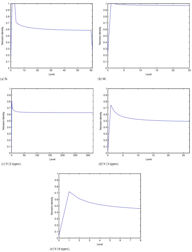
lmatrices are not necessarily very sparse (see

Fig. 2), we considered their full and sparse storages. If we exclude the change in the value of the nonzero density at the boundary level when going from 1 to 0 and observe the nonzero density’s value for l

≤

High

−

1, we see that it is at least 45% and attained by the V-model with 4 type of customers (seeFig. 2(e)).

In order to computeR

˜

l, we need to obtain the nonzero blocks Ql+1,l+1and Ql+2,l+1of Q , form Alby multiplyingR

˜

l+1with

Ql+2,l+1, and then add Ql+1,l+1to the product. At the end, Alshould be LU factorized and the linear system solved for each right-hand side vector in Bl. The matrix–matrix multiplicationR

˜

l+1Ql+2,l+1can proceed in two different ways. First, Ql+2,l+1

may be generated from the Kronecker representation as a sparse matrix and the pre-multiplication withR

˜

l+1performed.

Second, the efficient vector-Kronecker product algorithm [4,28] can be used to multiply rows ofR

˜

l+1with Ql+2,l+1while the

latter operand is being held in Kronecker form.

When theR

˜

lmatrices are chosen to be stored as full matrices, a temporary matrix in full storage needs to be kept to form

Aland then compute its LU factorization in place. SinceR

˜

High

=

0, the sparsity pattern of AHigh−1is equal to that of QHigh,High. Therefore, it makes sense to obtainR

˜

High−1using sparse LU factorization even though it will be stored as a full matrix. Now,

although all theR

˜

lmatrices should be kept until the end of the computation to obtain the steady-state solution and the sizes of the matrices are known at the outset (i.e.,R

˜

lis (

|

S(l)

| × |

S(l+1)

|

) and Alis (

|

S(l+1)

| × |

S(l+1)

|

)), it is still possible to use two different memory allocation–deallocation schemes for theR

˜

lmatrices and the temporary matrix. First, memory to store all

˜

Rlmatrices from l

=

High

−

1 down to Low and the largest temporary matrix, AHigh−1, can be allocated at the outset and

deallocated at the end of the computation. In this scheme, successive Almatrices will overwrite the same temporary matrix. Second, it is possible to deallocate the memory of Alat the end of step l and allocate the memory forR

˜

l−1and Al−1at the

beginning of step

(

l

−

1

)

. When the temporary matrix is allocated once at the beginning of the program, peak total memory usage is higher especially when nIis larger. SeeTable 2in which peak total memory usage values are computed analytically in Megabytes (MB) using the sizes of the matrices across all models for the full storage ofR

˜

l matrices,R

˜

l matrices plus temporary matrix AHigh−1at the outset, andR

˜

lmatrices plus Alat each level. In the next section, these analytically obtained values will be used to verify the memory usage measurements in the numerical experiments. On the other hand, when the

(12)

(a) N. (b) W.

(c) V (2 types). (d) V (3 types).

(e) V (4 types).

Fig. 2. Nonzero densities ofR˜lmatrices at levels l=0. . . ,High−1 for the call center models.

˜

Rlmatrices are chosen to be stored as sparse matrices, the temporary matrix to form Alis also stored as a sparse matrix and memory is allocated at each level. This implies that extra memory needs to be allocated for the sparse LU factorization of Al since there is expected to be fill-in.

We monitor the memory allocation of the LDQBD solver with the

pidstat

command of the

sysstat

package under Linux. This command returns the memory allocated by the program at run time in one second intervals. When theR

˜

lmatrices