© TÜBİTAK
doi:10.3906/elk-2001-123 h t t p : / / j o u r n a l s . t u b i t a k . g o v . t r / e l e k t r i k /
Research Article
Controlling a launch vehicle at exoatmospheric flight conditions via adaptive
control allocation
Yıldıray YILDIZ∗
Mechanical Engineering Department, Faculty of Engineering, Bilkent University, Ankara, Turkey
Received: 25.01.2020 • Accepted/Published Online: 11.04.2020 • Final Version: 29.07.2020
Abstract: The focus of this paper is the control of a reusable launch vehicle at exoatmospheric flight conditions, in the presence of actuator effectiveness uncertainty. Since during exoatmospheric flight, dynamic pressure is nonexistent, aerodynamic control surfaces cannot be used. Under these conditions, reaction control jet actuators can provide the necessary thrust to control the vehicle. Reaction control jets have only 2 states, namely, on and off, and continuous control inputs can be implemented with the help of pulse width modulation, which is also employed in this paper. A continuous controller is designed in the outer loop and a control allocator is used to distribute the total control input among redundant actuators, whose effectiveness are assumed to be unknown. The unknown actuator effectiveness is addressed with the help of an adaptive control allocator. A representative model of a reusable launch vehicle equipped with reaction control jets is used to demonstrate the effectiveness of the overall control scheme.
Key words: Adaptive control allocation, reaction control jets, reusable launch vehicles
1. Introduction
At exoatmospheric conditions, the conventional aerodynamic control surfaces cannot be used since forces and moments cannot be generated in the absence of dynamic pressure. Reaction control jets (RCJ) and reaction
wheels are generally the main actuators under exoatmospheric conditions [1]. In this paper, the focus is on the
attitude control of a launch vehicle equipped with only RCJs. RCJs provide thrust in only 1 direction and have 2 states, namely on and off, which put them in the category of pulsed actuators.
A control system can treat RCJs as continuous actuators, with the help of pulse modulation, or they can be used with a bang-bang control approach, where the jets are fired on and off based on a phase-plane analysis
[2]. Implementation of both of these approaches can be found in the open literature. Phase-plane based on-off
control using RCJs is employed for the Apollo command module [3], Mars Science Laboratory [4], Space Shuttle
[5] and Near Earth Asteroid Scout CubeSat [6], to name a few. To address the multiaxis coupling problem,
which is challenging to handle using the phase-plane analysis, an alternative mixed-integer linear programming
formulation is proposed in [7], where RJCs are blended together with aerodynamic control surfaces. Examples
of pulse modulation based approaches utilizing RCJs can be found in [8–11].
Control allocation (CA) is a method used to distribute the desired total control effort produced by a controller to redundant actuators. There exist several different approaches to achieve this task. One way to allocate redundant actuators is to use the pseudo-inverse of the input matrix to produce individual actuator
signals [12–14]. Another method is defining a cost function as a difference between the desired and achieved
∗Correspondence: [email protected]
control signals and using optimization techniques to minize this function [15–17]. In general, a secondary function, such as radar signature or drag minimization is also achieved in these optimization based methods,
by adding additional terms to the cost function. A survey on various types of CA can be found in [18].
In this study, a control allocation based control framework is proposed for launch vehicles equipped with RCJs controlled using pulse width modulation (PWM). What distinguishes this work from existing studies is that the RCJ control effectiveness is assumed to be unknown. The control effectiveness may decrease due to wear and tear, as well as the thruster gas pressure loss after long periods of use. To address this problem, a
control structure inspired by a recently developed adaptive control allocator [19,21] is used.
To summarize, the contributions of this study are 2 folds: First, a control framework for RCJ equipped
launch vehicles is proposed, where the RCJ dynamics are uncertain. Secondly, different from [19, 21] the
effectiveness of the adaptive control allocation algorithm is demonstrated in a setting where the actuators are controlled via PWM. In the simulation studies, it is shown that even when the actuators experience a dramatic loss of effectiveness, the proposed control framework is capable of providing a reasonable closed loop performance.
The organization of the paper is as follows. In Section2, the necessary background to follow the technical
developments in the paper is provided. In Section 3, the dynamics of the vehicle to be controlled is given. The
overall control framework is presented in Section 4, where the controller, the control allocator and pulse width
modulation is discussed. Simulation results are given in Section 5, where a comparison with a conventional
optimal control allocator is provided. Finally, a summary and discussion of the paper is given in Section 6.
2. Preliminaries
In this section, the projection operator is introduced, following the description given in [20], which is used later
in the technical development of this study.
Considering vectors θ∈ ℜn and y∈ ℜn, and a convex and smooth function, f (·), the projection operator
is given, using the gradient operator, ∇, as
Proj(θ, y)≡
{
y−∇f(θ)(∇f(θ))||∇f(θ)||2 Tyf (θ) if f (θ) > 0 and y
T∇f(θ) > 0
y otherwise. (1)
The operator can also be defined for matrices, instead of vectors, as Proj(Θ, Y ) = (Proj(Θ1, Y1), ..., Proj(Θm, Ym)) .
Here, Θi and Yi, i=1,...,m, refer to the ith columns of the matrices Θ and Y , and the projection applied on
these columns are defined in (1).
Projection operator can also be implemented elementwise: For a ∈ ℜ and b ∈ ℜ, which may be
considered, for example, as components of the vectors Θi and Yi, the projection operator is defined as
Proj(a, b)≡
{
b− bf(a) if f (a) > 0 and b(df (a)/da) > 0
b otherwise. (2)
Defining ϵ ∈ ℜ+ as the projection tolerance, and a
min and amax as the lower and upper bounds of a , the
convex function f (·) in (2) can be defined as
f (a) = (a− amin− ϵ)(a − amax+ ϵ) (amax− amin− ϵ)ϵ
The following 2 properties [20] of the projection algorithm makes it a useful tool to obtain a stable closed loop system in adaptive control applications.
Property 1 Given that a(0) ∈ A = {a ∈ ℜ|f(a) ≤ 1}, where a(0) is the initial condition of a(t) and f (a) :ℜ → ℜ is a convex function, if ˙a(t) =Proj(a, b), then a ∈ A for all t ≥ 0. It is noted that this property is used to guarantee the boundedness of the adaptation parameters independently from the stability of the overall system dynamics.
Property 2 Given a∗ ∈ [amin+ ϵ, amax− ϵ], where a ∈ ℜ and b ∈ ℜ are the components of the columns
Θi and Yi, i=1,...,m, of the matrices Θ∈ ℜn×m and Y ∈ ℜn×m, if the projection algorithm (2) with (3) is
implemented, then the inequality
tr((ΘT − Θ∗T)(Proj(Θ, Y )− Y ))≤ 0 (4)
holds, where the trace operation is referred to as tr(·).
3. Plant dynamics
In this study, a representative mathematical model for a reusable launch vehicle investigated in [7] is used to
demonstrate the effectiveness of the proposed control framework. A brief description of the model is given in this section.
Consider the equation of motion
M = J ˙ω, (5)
where M ∈ ℜ3 is the net moment acting on the vehicle, J ∈ ℜ3×3 is the inertia matrix, and ω ∈ ℜ3 is
the angular velocity vector, consisting of roll, p , pitch, q , and yaw, r , rates. Assuming small angles, it is
obtained that ˙ϕ = p , ˙θ = q , and ˙ψ = r , where ϕ , θ , and ψ are the Euler angles. Defining the state vector as
x = [p, ϕ, q, θ, r, ψ]T, (5) can be represented in state-space form as ˙ x = Ax + BMM y = Cx, (6) where A = 0 1 0
0
0 0 0 0 0 1 0 0 0 0 0 0 0 0 0 0 1 0 , B = Ixx−1 0 0 0 0 0 0 Iyy−1 0 0 0 0 0 0 Izz−1 0 0 0 , C = 00 10 00 01 00 00 0 0 0 0 0 1 . (7)In (7), Ixx∈ ℜ+, Iyy ∈ ℜ+ and Izz ∈ ℜ+ are the vehicle moment of inertias calculated along the main axes.
The net moment, M , is created with the help of RCJs. Assuming that there exists n RCJs, and given a
mapping matrix T ∈ ℜ3×n, the net moment can be calculated as
where u ∈ ℜn represents the RCJs’ output vector, each element of which can be treated as a real number between 0 and 1, with the help of PWM. Since it is assumed that the thrusters’ effectivenesses are unknown, a
diagonal matrix with positive elements, Λ∈ ℜn×n, is introduced to (8) as
M = T Λu. (9)
It is noted that Λ is unknown and represents uncertain actuator effectiveness.
4. Control system design
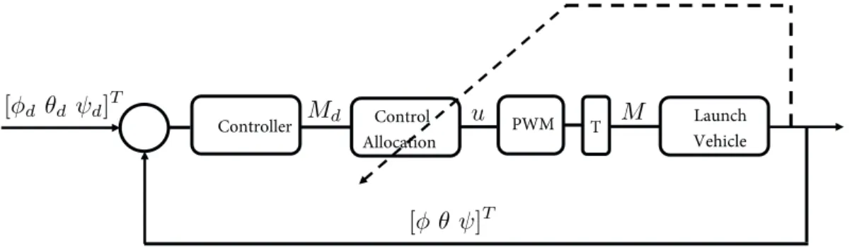
Overall closed loop system structure, including the launch vehicle, controller and the control allocator, together
with the pulse-width-modulation (PWM) and the torque matrix, T , is shown in Figure1. Below, the working
principles of these individual components are explained.
Control Allocation
Controller PWM Launch
Vehicle T
Figure 1. Overall closed loop system structure.
4.1. Controller
The outer loop controller assumes a plant dynamics without any uncertainties, given in (6). The uncertainties
are handled by the adaptive control allocator, which is explained in the following sections. For the outer loop
controller, the controller proposed in [7] is used, which produces decoupled second order dynamics for the roll,
pitch and yaw channels, with a damping ratio of 0.7 and a natural frequency of 3 rad/s. Defining the desired
orientation of the launch vehicle with ϕd, θd and ψd, to obtain the decoupled dynamics, the control signal is
calculated as Md=−J 4.20 90 4.20 09 00 00 0 0 0 0 4.2 9 x + J 90 09 00 0 0 9 ϕθdd ψd . (10)
It is noted that Md in (10) consists of the desired values of the moments M in (6). These desired values are
realized by the control allocator, which is explained in the following section.
4.2. Control allocator
The goal of the control allocator is to receive the control signal, Md, and realize this signal using n different
RCJs, in the presence of thruster effectiveness uncertainty, represented by Λ in (9). Inspired from [21], to
achieve this goal, the problem is defined in the model reference adaptive control domain.
Assuming a stable, 3-by-3 matrix, Am, consider the dynamics
˙
and a reference model
˙
zm= Amzm. (12)
Representing the parameter matrix to be determined as Θ∈ ℜ3×n, RCJ output vector, u, is created as
u = ΘTMd. (13)
Substituting (13) into (11), it is obtained that
˙
z = Amz + (T ΛΘT− I)Md. (14)
To continue the technical development, it is assumed that an ideal parameter matrix Θ∗ exists such that
T ΛΘ∗T = I, (15)
where I is the identity matrix with appropriate dimensions. Defining ez = z− zm and ˜Θ = Θ− Θ∗, where
˜
Θ can be considered as the deviation from the ideal parameter matrix, and subtracting (12) from (14), it is
obtained that
˙ez= Amez+ T Λ ˜ΘMd. (16)
The adaptation law is obtained by conducting a Lypunov stability analysis, using a Lypunov function candidate
V = eTzP ez+ tr( ˜ΘTΘΛ),˜ (17)
where P is the solution of the Lyapunov equation AT
mP + P Am=−Q. Here, Q can be taken as any positive definite symmetric matrix, which also makes the solution P symmetric and positive definite. Taking the
derivative of (17) using (16), and the Lyapunov equation, it is obtained that
˙
V =−eTzQez+ 2eTzP T Λ ˜ΘT Md+ 2tr( ˜ΘTΘΛ).˙˜ (18)
Exploiting the property xTy = tr(yxT) , where x∈ ℜn and y∈ ℜn, (18) can be rewritten as
˙ V =−eTzQez+ 2tr (˜ ΘT(MdeTzP T +Θ)Λ˙˜ ) . (19)
Noting that ˙Θ =Θ , if the adaptation law˙˜
˙
Θ = Proj(Θ,−MdeTzP T ) (20)
is used, (19) can be rewritten as
˙ V =−eTzQez+ 2tr (˜ ΘT(MdeTzP T + Proj(Θ,−MdeTzP T ))Λ ) . (21)
Using Property 2, given in Section 2, it can be shown that ˙V ≤ 0. Then, with the help of Barbalat’s lemma
[22], it is obtained that limt→∞ez(t) = 0 , assuming that Md is bounded. Boundedness of Md can be obtained
4.3. Pulse width modulation
The control allocator determines the individual RCJ outputs (13) to realize the control signal (10), employing
the adaptation rule (20). Since RCJs have only 2 discrete states, on and off, the continuous output vector, u ,
requested by the control allocator is achieved with the help of pulse-width-modulation (PWM) (see Figure 1).
To provide meaningful input signals to the PWM, the elements of u should be bounded in the interval [0, 1].
However, to facilitate the design of the adaptive law (20), a symmetric saturation limit, [-1,1] is defined for u .
It is noted that this introduces additional uncertainty to the overall control system, which is expected to be handled by the adaptive control allocation.
Once the limits of u are set, the attainable moments can be obtained using the relationship (8). The
limits of the attainable moment set are then set as the saturation limits for the controller output Md. Using
these saturation limits and (13), the boundaries of the parameter matrix Θ elements can be calculated, which
can be enforced using the projection algorithm.
The PWM used in the tests has a cycle time of 80 ms. The simulation step time is set to be 8 ms.
5. Simulation results
During the simulations, a continuous reference vector [ϕd, θd, ψd] is provided to the closed loop system. The
controller produces the desired moment vector Md. The control allocator then produces the necessary actuator
input signal vector, u, which is realized by PWM. The moment vector created by RCJs on the vehicle is then
calculated via (9), using the mapping matrix T , given as [7]
T = −3670 −15110 −69828574 −50988702 −3670 15150 −6981 8702−8573 5098 −3670 −3670 14675 −11597 −6981 −8702 −14675 11597 6981 8702 −14675 14675 . (22)
It is noted that each entry of the matrix T represents the moment produced by the corresponding RCJ. To introduce actuator uncertainty to the moment calculation, the actuator effectivenesses are reduced to 30 % of their full capacity, at t = 20 s, employing the actuator effectiveness matrix Λ .
The adaptive control allocation solution is compared with a conventional optimal control allocation method in the following sections. Before the comparison results are given, the parameter initialization process for both control allocators are explained below.
5.1. Initialization of the control allocation parameters
The adaptive control allocator’s parameter matrix is updated online using the adaptive law given in (20).
The initial conditions for this parameter matrix can be selected as zero, if one does not prefer to use any prior knowledge about the plant. In the simulation studies conducted in this paper, the initial conditions for
this matrix is calculated using (15), where the uncertainty matrix Λ is taken to be an identity matrix, since
fault/uncertainty identification is not done in this work. Defining ¯Θ ≡ Θ(0), this initial condition selection
creates a control allocation output that is equivalent to
u = ¯ΘTMd+ ΘTMd, (23)
where the first term is a fixed actuator signal and the second term acts as an adaptive augmentation whose adaptive parameter matrix elements are initialized to zero.
The initial parameter values obtained by setting Λ = I , where I is an identity matrix, and solving (15), are also the ideal values for the optimal control allocation, which is explained in the next section. Therefore the same initial values are used for the optimal control allocator.
5.2. Comparison with an optimal control allocation method
In optimal control allocation, the objective function
f (u) =||T u − Md||22+||u|| 2
2 (24)
is minimized while ensuring 0≤ u ≤ 1.
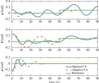
Figure 2 shows the tracking curves for the optimal and adaptive control allocators. Although a severe
anomaly, such as a 70 % actuator effectiveness loss, is introduced, adaptive control allocator still provides a reasonable performance. Optimal control allocator, on the other hand shows long standing oscillations, especially in the roll, ϕ , channel.
0 10 20 30 40 50 60 70 80 90 -0.2 0 0.2 0.4 [ra d] 0 10 20 30 40 50 60 70 80 90 -0.2 0 0.2 0.4 [ra d] 0 10 20 30 40 50 60 70 80 90 time [s] -0.4 -0.2 0 0.2 [ra d] Optimal CA Adaptive CA Reference
Figure 2. Attitude tracking performances of the optimal and adaptive control allocators.
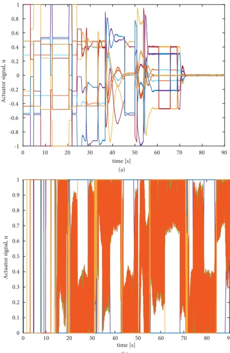
The advantage of using adaptive control allocator becomes more apparent when the actuator signals
are compared. As seen in Figure 3, the actuator signals produced by the optimal control allocator have high
frequency oscillations, while the ones produced by the adaptive control allocator show reasonable switching times.
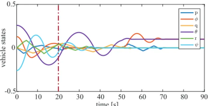
Finally, the evolution of all vehicle states, p, ϕ, q, θ, r and ψ , are presented in Figure4. Even though a
large uncertainty is introduced at t = 20 s, which is marked on the figure, all the states remain bounded within reasonable bounds and converge to constant values within a reasonable time interval.
6. Summary and discussion
In this paper, a control allocation solution is proposed for the control of launch vehicles in exoatmospheric conditions. There exist 2 main challenges for this task. The first challenge is controlling the system in the presence of actuator uncertainty. The second challenge is the specific characteristics of the reaction control jet (RCJ) actuators, which provide only on and off modes of operation, either providing a constant amount
0 10 20 30 40 50 60 70 80 90 time [s] -1 -0.8 -0.6 -0.4 -0.2 0 0.2 0.4 0.6 0.8 1 Act uato r signal ,u (a) 0 10 20 30 40 50 60 70 80 90 time [s] 0 0.1 0.2 0.3 0.4 0.5 0.6 0.7 0.8 0.9 1 Act uato r signal ,u (b)
Figure 3. Actuator signals produced by the adaptive control allocator (a), and by the optimal control allocator (b). of trust or not providing any input. The first challenge is addressed by the adaptation capability of the investigated control allocation algorithm. A common approach to remedy the second challenge is using pulse-width modulation (PWM), which enables the designer to treat the control signals as continuous duty-cycle commands. To achieve this, the control allocation output must be constrained properly. In the presented control allocation method, this is achieved using the projection algorithm. It is demonstrated that the exploited adaptive control allocation method performs better than a conventional optimal control allocator in the presence of actuator uncertainty.
Although the simulation results show the advantage of using an adaptive approach compared to a nonadaptive method, there is a large room for improvement for the presented adaptive control allocation
0 10 20 30 40 50 60 70 80 90 time [s] ve hi cl e s ta te s -0.5 0 0.5
Figure 4. Evolution of vehicle states when the adaptive control allocation is employed.
method. For example, instead of using a symmetric projection boundary, an asymmetric boundary can be used to eliminate the additional uncertainty introduced to due negative control allocation outputs. Another improvement would be designing the control allocator for the RCJs’ 2-state output (on/off ), instead of using an approximate method such as PWM. This paper presents a first attempt at attacking the problem of controlling a vehicle with RCJs using adaptive control allocation, and the discussed improvements will be considered in future work.
Acknowledgment
This work is supported by the Young Scientists Award Programme of the Turkish Academy of Sciences.
References
[1] Song G, Agrawal BN. Vibration suppression of exible spacecraft during attitude control. Acta Astronautica 2001; 49 (2): 73-83. doi: 10.1016/S0094-5765(00)00163-6
[2] Bryson AE. Control of Spacecraft and Aircraft. Princeton, New Jersey: Princeton University Press, 1993.
[3] MIT Charles Stark Draper Laboratory. Guidance System Operations Plan for Manned CM Earth Orbital and Lunar 6 Missions Using Program Colossus 3. Section 2: Data links. Washington, DC, USA: NASA, Technical Report R-577, 1970.
[4] Calhoun PC, Queen EM. Entry vehicle control system design for the mars science laboratory. Journal of Spacecraft and Rockets 2006; 43 (2): 324-329. doi: 10.2514/1.19650
[5] Hattis P, Kubiak E, Penchuk A. A frequency domain stability analysis of a phase plane control system. Journal of Guidance, Control, and Dynamics 1985; 8 (1): 50-55. doi: 10.2514/3.19934
[6] Stiltner BC, Diedrich B, Becker C, Bertaska I, Heaton AF et al. Cold gas reaction control system for the near earth asteroid scout cubesat. In: AIAA SPACE and Astronautics Forum and Exposition; Orlando, FL, USA; 2017. pp. 1-17.
[7] Doman DB, Gamble BJ, Ngo AD. Quantized control allocation of reaction control jets and aerodynamic control surfaces. Journal of Guidance, Control, and Dynamics 2009; 32 (1): 13-24. doi: 10.2514/1.37312
[8] Paradiso JA. Adaptable method of managing jets and aerosurfaces for aerospace vehicle control. Journal of Guidance, Control, and Dynamics 1991; 14 (1): 44-50. doi: 10.2514/3.20603
[9] Wie B, Murphy D, Paluszek M, Thomas S. Robust attitude control systems design for solar sails (part 2): microppt-based backup acs. In: AIAA Guidance, Navigation, and Control Conference and Exhibit; Rhode Island, USA; 2004. pp. 1-16.
[10] Jeon SW, Jung S. Novel limit cycle analysis of the thruster control system with time delay using a pwm-based pd controller. In: IEEE International Symposium on Industrial Electronics; Seoul, South Korea; 2009. pp. 1245-1250.
[11] Li J, Gao C, Jing W, Wei P. Dynamic analysis and control of novel moving mass flight vehicle. Acta Astronautica 2017; 131: 36-44. doi: 10.1016/j.actaastro.2016.11.023
[12] Durham WC. Constrained control allocation. Journal of Guidance, Control, and Dynamics 1993; 16 (4): 717-725. doi: 10.2514/3.21072
[13] Alwi H, Edwards C. Fault tolerant control using sliding modes with on-line control allocation. Automatica 2008; 44 (7): 1859-1866. doi: 10.1016/j.automatica.2007.10.034
[14] Tohidi SS, Sedigh AK, Buzorgnia D. Fault tolerant control design using adaptive control allocation based on the pseudo inverse along the null space. International Journal of Robust and Nonlinear Control 2016; 26 (16): 3541-3557. doi: 10.1002/rnc.3518
[15] Petersen JA, Bodson M. Constrained quadratic programming techniques for control allocation. IEEE Transactions on Control Systems Technology 2005; 14 (1): 91-98. doi: 10.1109/TCST.2005.860516
[16] HäRkegåRd O, Glad ST. Resolving actuator redundancy: optimal control vs. control allocation. Automatica 2005; 41 (1): 137-144. doi: 10.1016/j.automatica.2004.09.007
[17] Casavola A, Garone E. Fault-tolerant adaptive control allocation schemes for overactuated systems. International Journal of Robust and Nonlinear Control 2010; 20 (17): 1958-1980. doi: 10.1002/rnc.1561
[18] Johansen TA, Fossen TI. Control allocation a survey. Automatica 2013; 49 (5): 1087-1103. doi: 10.1016/j.automatica.2013.01.035
[19] Tohidi SS, Yildiz Y, Kolmanovsky I. Fault tolerant control for over-actuated systems: An adaptive correction approach. In: American Control Conference; Boston, MA, USA; 2016. pp. 2530-2535.
[20] Lavretsky E, Gibson TE. Projection operator in adaptive systems. arXiv preprint 2011; 1112.4232.
[21] Tohidi SS, Yildiz Y, Kolmanovsky I. Model reference adaptive control allocation for constrained systems with guaranteed closed loop stability. arXiv preprint 2019; 1909.10036.