An application of seasonal cointegration and error correction models on monthly data

е ж

M D

».

f

_ s

T!'

X

f: -ß

5 ■<*

5*і і й і.іШ ё f e É f c э ! i S » ô f f i l e s

asá íl!§ te^'îö'Ss sf bt iiçéfâ a é Штш S afeess &f

S î l k è i t

Ш PBJfй

f t tfes Іш рігм ^^й:

« - - ’ЧІ Ü « - w -« i.' ^ Ч» ■ , >íl»' w · *.

?■ Я Д C "f* c o

_{I v.'^ .•■*^.. * ' i ■^'^'}

V

_{' *’}

f^T i> ·'.·; ■

>

.Ц

4j.'

‘•■- '■ A 'i#· ^5

S 7 0 é S

AN APPLICATION OF SEASONAL COINTEGRATION AND

ERROR CORRECTION MODELS ON MONTHLY DATA

A Thesis

Submitted to the Department of Economics

and the Institute of Economics and Social Sciences o f

Bilkent University

In Partial Fulfillment o f the Requirements

for the Degree o f

MASTER IN ECONOMICS

by

Gtiliz ERCO§KUN

July 1995

и &

Б Я О С о . Б . I г Б

I certify that I have read this thesis and in my opinion it is fully adequate, in scope and in

quality, as a thesis for the degree of Master in Economics.

Asist. Prof. Dr. Kıvılcım Metin

I certify that I have read this thesis and in my opinion it is fully adequate, in scope and in

quality, as a thesis for the degree of Master in Economics.

1

(.

//

Prof. Dr. As^ad 2[aman

I certify that I have read this thesis and in my opinion it is fully adequate, in scope and in

quality, as a thesis for the degree of Master in Economics.

Approved by the Institute of Social and Economic Sciences

Director:

ABSTRACT

AN APPLICATION OF SEASONAL COINTEGRATION AND ERROR CORRECTION M ODELS ON M ONTHLY DATA

Gûliz Ercoşkun M in Economics

Supervisor: Asist. Prof. Dr. Kivdcun Metin June 1995

In this study, I try to analyze and show the monthly changes and their effects on each other o f Istanbul Stock Exchange (ISE), TL / $ Exchange Rate (E), M l, M2, price level (P), Interest rate on securities (R) and Advances o f the central bank to the treasury (A) by developed techniques in time series econometrics, namely unit roots, seasonal cointegration and error correction. The long run relationship between stock prices and exchange rate, price level. M l, M2 investigated by using these techniques o f time series. Conclusions are made for future use o f models for monthly time series. To our knowledge, this is among the pioneering studies conducted in an emerging m arket that uses an updated econometric methodology to allow for an analysis o f monthly data for long run steady state properties together with short run dynamics.

Key W o rd s: Unit Root, Seasonal Cointegration, E rror Correction, Istanbul Stock Exchange.

ÖZET

M EVSİM SEL KOİNTEGRASYON V E H A TA DÜZELTM E M ODELLERİNİN AYLIK VERİLER ÜZERİNE UYGULANM ASI

Güliz Ercoşkun Yüksek Lisans Tezi

Tez Yöneticisi; Yrd. Doç. Dr. Kıvılcun Metin Temmuz 1995

Bu tez Türkiye’de 1986-1994 dönemindeki İstanbul M enkul Kıymetler Borsası, döviz kuru (TL\$), M İ, M2, enfilasyon, avans ve hazine bonosu faiz oranlan arasmdaki ilişkileri aylık veriler göz önüne almarak incelemektedir. Ekonom etrik olarak, zaman serileri kullanılarak aybk veriler için mevsimsel kointegrasyon ve hata düzeltme modelleri türetilmiştir. Bu çalışma, bu konuda aylık veriler baz almarak hazırlanmış öncü çalışmalardan birisidir.

A n a h ta r K elim eler: Birim kök. Mevsimsel Kointegrasyon, Hata Düzeltme, İstanbul Menkul Kıymetler Borsası

ACKNOWLEDGMENTS

I am grateful to Asist. Prof. Dr. Kivilcim Metin for her supervision and guidance throughout the development o f this thesis.

CONTENTS

1. In tro d u ctio n

Page

1.1 Introduction 1.2 The Settings 1.3 The Data Set

1

3

6

2. Seasonality

2.1 Definition

2.2 Importance o f Right Augmentation 2.3 Testing Procedure

2.4 Influence o f Deterministic Components to the Test

3. Seasonal Cointegration for Monthly Series

3.1 Definition

3.2 Testing Procedure

4. Error Correction Representation for Monthly Series

4.1 Definition 4.2 Testing Procedure

5. Results

6. Conclusion

References

8 10 13 22 24 26 37 39

46

55 APPENDIX A 1. Data

APPENDICES

Table 1( Data for A, monthly, 86M1-94M5 ) Table 2( Data for ISE, monthly, 86M 1-94M12 ) Table 3( Data for E, monthly, 86M1-94M12 ) Table 4( Data for M l, montldy, 86M1-94M12 )

Table 5( Data for M2, monthly, 86M 1-94M12 ) Table 6( Data for P, monthly, 86M 1-94M12 ) Table 7( Data for R, monthly, 86M1-94M5 )

2. Results o f Seasonal Frequency Calculations, ‘t ’ and ‘F ’ statistics Table 8( Seasonal Frequency Calculation Results for I S E ) Table 9( Seasonal Frequency Calculation Results for R ) Table 10( Seasonal Frequency Calculation Results for M2 ) Table 11( Seasonal Frequency Calculation Results for M l ) Table 12( Seasonal Frequency Calculation Results for A) Table 13( Seasonal Frequency Calculation Results for P ) Table 14( Seasonal Frequency Calculation Results for E ) 3. Results o f Cointegration and Error Correction Tests

Table 15( Results o f Cointegration Tests between ISE and E) Table 16( Results o f Cointegration Tests between ISE and M l) Table 17( Results o f Cointegration Tests between ISE and M 2) Table 18( Results o f Cointegration Tests between ISE and P) Table 19( Results o f Error Correction M odels between ISE and E) Table 20( Results o f Error Correction Models between ISE and M l) Table 21( Results o f Error Correction M odels between ISE and M 2) Table 22( Results o f Error Correction M odels between ISE and P)

APPENDIX B 1. Graphs

G raphl ( A for years between 86M1-94M5) Graph2 ( A y It for years between 87M1-94M5) Graph3 ( A y5t for years between 87M1-94M5) Graph4 ( A y6t for years between 87M1-94M5) Graphs ( ISE for years between 86M1-94M12) Graph6 ( ISE y It for years between 87M1-94M12) Graph7 ( ISE ySt for years between 87M1-94M12) Graph8 ( ISE y6t for years between 87M 1-94M12) Graph9 ( E for years between 86M1-94M12) G raphic ( E y It for years between 87M1-94M12) G raphl 1 ( E ySt for years between 87M 1-94M12) G raphl2 ( E y6t for years between 87M 1-94M12) G raphl3 ( M l for years between 86M1-94M12) G raphl4 ( M l y It for years between 87M 1-94M12) GraphlS ( M l ySt for years between 87M1-94M12) G raphic ( M l y6t for years between 87M1-94M12

GraphlV (M 2 for years between 86M1-94M12) G raphlS (M 2 y It for years between 87M1-94M12) G raphl9 (M 2 y5t for years between 87M1-94M12) Graph20 (M 2 y6t for years between 87M1-94M12) Graph21 ( P for years between 86M1-94M12) Graph22 ( P y It for years between 87M1-94M12) Graph23 ( P y5t for years between 87M1-94M12) Graph24 ( P y6t for years between 87M1-94M12) Graph25 ( R for years between 86M1-94M12) Graph26 ( R y I t for years between 87M1-94M12) Graph27 ( R y5t for years between 87M1-94M12) Graph28 ( R y6t for years between 87M1-94M12)

CHAPTER 1

1.1 INTRODUCTION

An important set o f information which is ignored in the efficient m arket literature - with only a few exceptions - is the information revealed by m acroeconomic variables. Fama (1991) concludes his well known review article on efficient markets by encouraging research that “relates the behavior o f expected returns to the real economy”. Macroeconomic variables constitute a relatively m ore important set o f information in thin markets in comparison to mature ones. In thin markets, the volume o f trade is relatively low, and pubhcity available information on company performances is generally limited and untimely. Also, most o f the thin markets are operational in developing countries where capital accumulation and economic activity is initiated by the state. Therefore, the thinly traded stock markets o f controlled economies are expected to absorb fiscal and monetary changes as important sets o f information.

The conventional methodology employed in this field o f research, briefly reviewed above, is based on the use o f time series regression. The development o f seasonal cointegration theory in econometrics permits a long-run analysis o f the nonstationary time series to study the relationship between stock returns and macroeconomic variables, using an error correction m odel o f stock prices and testing for the seasonal cointegrating relation between stock prices and the variables o f interests.

In this study, I try to test the relationships between Istanbul Stock Exchange (ISE) and price level (P), M l, M2, Interest Rates (R), Advances o f central bank to treasury (A), Turkish Lira-dollar exchange rate (E) by using the time series analysis namely, seasonal cointegration and error correction. To our knowledge, this is among the pioneering studies conducted in an emerging m arket that uses an updated econometric methodology to allow for an analysis o f long run steady state properties together with short run dynamics for monthly data.

Accordingly, the thesis is organized as follows. After presenting a brief description o f unit root, seasonal cointegration, I deal with seasonal cointegration and error correction theory for monthly data for Istanbul Stock Exchange and other variables. First o f all, the variables which are used are driven, then the Hylleberg-Engle-Granger-Yoo (HEGY) model for quarterly data improved and made useful for monthly data. Then these tests are used to test the cointegration relationships among the variables. The existence o f long run equihbrium relations w ere tested by updated version o f Engle and Granger (1987) tw o- step approach, Frances (1991) seasonality approach and HEGY (1990) seasonal cointegration and error correction approach, but here I w ant to point out again that these models are updated for monthly case. Evidence is provided for long run movements o f macro-economic variables and stock prices as well as their short run behavior. Finally, conclusions are made and a very useful method for testing o f seasonal cointegration and error-correction models for time series are derived for monthly case.

1.2 THE SETTINGS

Turkey for m ore than a decade has functioned as a good case study for the set o f developing and post-communist coxmtries in the process o f structural change and hberalization. Stmctural change from a government - regulated economic regime to a market-oriented one commenced with the economic package introduced in January 1980. Main topics o f the poHcies were the convertibihty o f the Turkish lira, flexible exchange rate pohcy and export promotions. As a component o f the program, there was a major devaluation o f Turkish lira in January 1980. The 1980 program also included some interest rate pohcy, which lead interest rates exceed inflation rate. As a result o f these pohcies in

1981-1983 period, the inflation rate did not exceed 36%.

In the period 1984-1987, the average inflation rate was aroimd 40%. hi April 1986, the Central Bank set up an Interbank m arket for one and two week maturities and introduced overnight transaction in May 1986. In 1986, the Central Bank introduced for the first time the pohcy approach o f targeting a m onetary aggregate. M oney in wider sense (M 2) was selected to be kept on a growth path during the year. In 1986, M2 grew 38.6%, which was close to the target level. In 1986, M l had a growth o f 62.5% and reserve money had a growth o f 32.8% and the consumer price inflation achieved 34.6%. For 1987 the monetary authorities targeted growth o f M2 at 30 percent which was considered consistent with an expansion o f 5 percent and an inflation rate o f 25 percent. The central Bank planned 28 percent growth o f the reserve money which was the main instmment to control M2. But reserve money growth was nearly 50 percent in 1987 and

consumer price inflation was 38.9 percent. In 1987, M l growth was 58.3% and M2 growth was 37.6%.

hi view o f accelerating inflation and instahihty in financial markets, monetary pohcy was severely tightened in 1988. Deposit interest rates were raised to encourage financial savings and to reduce the share o f currency and sight deposits in M2. But, besides this tightening pohcy, targets were exceeded by substantial amount in 1988. M l, M2 and reserve money growth were 39.7%, 77.5% and 67.5%, respectively. Consumer price inflation reached 75.4% in 1988.

For 1989, the Central Bank has abstained fi:om announcing m onetary targets. In 1989, reserve growth accelerated due to increase in net foreign assets and due to the government’s decision to grant large salary increases and to raise agricultural support prices. Reserve money growth reached 75% and M l and M 2 growth w ere 97.1% and 82%, respectively. In 1989, consumer price inflation was at the level o f 69.9%. h i the context o f the program o f economic hberalization, the Turkish authorities have been ainting at placing greater rehance on monetary pohcy for economic stabilization purposes. However, as the Central Bank is not completely autonomous and economic pohcy decisions are taken at the governmental level, it has been difficult to follow a clear anti- ioflationary monetary pohcy.

Starting jfrom 1990, interest rate-exchange rate balance and foreign capital inflow

have directly depended on each other. In 1990 return fi'om interest was 2.5% above the

return from foreign currency and this caused 3000 million dollars o f foreign capital mflow. In 1991, the return from interest over return from foreign cmxency fell to -3.3% and this caused 3020 million dollars o f capital to leave the country. From this time after, return from interest have been always above the return from foreign currency and in 1992 and 1993 there have been seen net foreign capital inflow. In 1993, total Capital Movements item has reached 9279 milhon dollars and this value is 5.6% o f GNP in 1993.

Inflation has reached an average o f 68.2% in the period 1988-1992. Monetary pohcy aimed at maintaining orderly conditions in financial markets. The Central Bank, however, was again obhged to finance the PSBR, and hence fiscal imbalance induced rapid growth in monetary aggregates. In the period 1988-1992, M l, M2 and reserve money growth reached an average o f 62%, 67% and 58%, respectively.

Strong output growth in 1992 and 1993, led by domestic demand, brought about a widening current account deficit and rising foreign indebtedness. Inflationary pressures intensified, partly in response to further increase in pubhc sector deficits to very high levels. In 1993, real GNP growth averaged 6.75%, the trade deficit rose to 12% o f GNP and pubhc sector borrowing requirement (PSBR) rose to 16% o f GNP. Annual consumer price inflation averaged 66% in 1993, compared with 70% in 1992. At the end o f 1993, international credit worthiness was downrated and the Turkish lira drastically depreciated. M l, M2 and reserve money growth w ere 53%, 43% and 60%, respectively in 1993.

Starting in 1994, Turkish economy have undergone the m ost important crisis o f the last 15 years. The crises has started in the first months o f 1994 in finance m arket and it has spread to real part o f the economy in a httle time. The main causes o f the crises has been shown as the growing pubhc sector deficits and the incorrect steps tow ards Hberahzation.

For this period, consumer price inflation was 126%, and wholesale price inflation was 150% in 1994. Pubhc sector borrowing requirement fell to 8% o f GNP. In 1994, M l, M2 and reserve money growth reached 85%, 132% and 85%, respectively. In April 1995, the annual consumer price inflation achieved 94%. And in April 1995, the three months M l, M2 and reserve money growth ratios achieved 15.6%, 19.2% and 20%, respectively.

1.3 THE DATA SET

Our data set consists o f monthly observations for the period 1986:1-1994:12; all the observations are as the end o f period. Considering the macroeconomics o f the Turkish economy, w e have set the relations between stock returns and a set o f macroeconomic variables and I choose my variables according to this.

Stock returns are represented by the monthly index value o f the Istanbul Stock Exchange (ISE). Considering the relationship between inflation and the budget deficit (Metin, 1993,1994) this variable is included in the data set. Budget deficit is represented by the advances o f the central bank to the treasury (A) because the budget deficit is not announced on a monthly basis and these advances are widely used m the financial media as

indicators o f the annual budget deficit. Other variables are also chosen on the basis o f the availabihty and the higher firequency o f use o f information by the ultimate investors. Interest rates (R) are depicted by the monthly compounded value o f the three month treasury bill rate which is sensitive measure o f the “going rate o f interest” in the financial media. The Turkish Ura-U.S. dollar exchange rate (E) is also included in the data set due to the frequent open m arket operations o f the Central Bank using dollar reserves. Inflation (P) is measured by the consumer price index. Finally, money supply is represented by two monetary aggregates; M l which is ciuxency in circulation plus demand deposits and, M2 which is M l plus time deposits. All data are collected from several issues o f the Three Monthly Bulletin o f the Turkish Treasury. None o f the series are seasonally adjusted.

CHAPTER 2

2.1 DEFINITION

The rapidly developing time-series analysis o f models with unit roots has had a major impact on econometric practice and on omr understanding o f the response o f econometric systems to shocks.

Many economic time series contain important seasonal components and there are a variety o f possible models for seasonably which may differ across series. A seasonal series can be described as one with a spectrum having distinct peaks at the seasonal frequencies:

Ws = 27ijk / n where k = 0, 1 ,..., n-1, Ws are seasonal frequencies and n is the number o fp e rio d s in a y e a r.

Three classes o f time-series models are commonly used to m odel seasonably. These can be called;

(a) Purely deterministic seasonal process, (b) Stationary seasonal process,

A purely deterministic seasonal process Xt is a process generated by seasonal diunmy variable such as;

X i= P t, pt = mo + m iSi + m 2S2 + ... + mic-iSk-i k = number o f periods per year, mi = constants, Si = seasonals.

this process can be perfectly forecasted and wUl never change its shape.

A stationary seasonal process 'F(B ) can be generated by a potentially infinite autoregression.

'F(B)xt = 8i, 8t ~ i.i.d, independently identically distributed

with all o f the roots o f ^ ( B ) = 0 lying outside the unit circle but where some complex pairs with seasonal periodicities. M ore precisely, the spectrum o f such a process is given by;

f(w) = a^/1 'F (e’'^

f

where is some constant.

A series Xt is an integrated seasonal process if it has a seasonal imit root in its autoregressive representation. M ore generally, it is integrated o f order d at frequency 0 if the spectrum o f Xt, takes the form:

f(w) = c(w - 0)

-2d

for w near 0. This is conveniently denoted by:

Xi ~ le (d).

So, a series with a clear seasonal may be seasonally integrated, have a deterministic seasonal, a stationary seasonal, or some combination. A general class o f linear time-series models which exhibit potentially complex forms o f seasonality can be written as:

d(B) a(B) (xrl^t) = £t

where all the roots o f a(z) = 0 lie outside the unit circle, all the roots o f d(z) = 0 lie on the unit circle, and pt is some constant. Stationary seasonality and other stationary components o f Xt are absorbed into a(B), while deterministic seasonality is in pt when there are no seasonal unit roots in d(B).

2.2 IM PORTANCE OF RIGHT AUGM ENTATION

Suppose that each component o f Xt is 1(1) so that the change in each component is a zero mean pmely nondeterministic stationary stochastic process. Any known deterministic components can be subtracted before the analysis is begun. It follows that there will always exist a multivariate W old representation such that:

( l - B ) x t = C (B )8 t,

If we take to mean o f both sides, we will have the same spectral matrix. Further, C(B) will be uniquely defined by the conditions that the fimction det[C(z)], z = e*'^, have all zeroes on or outside the unit circle, and that C(0) = In, the N X N identity matrix. In this representation the St has zero mean white noise vectors with:

E[stSt'] = 0, 1 n , = G, t = n,

so that only contemporaneous correlations can occur.

Due to habit and convenience St is often assumed to be i.i.d. or n.i.d. It is quite easy to show that a process such as (1-B*^)yt = St or (1+B)yt = 8t has property that a process may alter the seasonal pattern completely. The definition o f integration does not require 8t to be anything else than stationary, in fact 8t can be bounded, heteroskedastic, autocorrelated conditional heteroskedastic, autocorrelated, nonsymmetric, etc. Due to the complex nature o f the economic system, i.e., o f the data-generating process 8 t , a simple univariate representation such as (1-B'^)yi = 8t may be expected to display such behavior. Such a univariate representation is therefore also best seen as an approximation that should be iaterpreted with care. Here an iategrated seasonal model is apphed to data with a varying seasonal pattern and the choice between a deterministic seasonal model and

integrated m odel depends on the degree o f variation the seasonal pattern.

The auxihary regression may be augmented by lagged values o f the dependent variable (1-B^^)yt = St without an efiect on the distribution imder the null as is the case with the Dickey - Fuller procedure. However, the pow er and size o f the test may depend critically on the ‘right augmentation being used. From Monte Carlo experiments w e know that the pow er o f Dickey-FuUer test suffers if too many auxihary parameters are appUed to render the errors white noise, while the size may be far greater than the chosen level o f significance if we use too few parameters. In addition one may add deterministic term s Uke an intercept, seasonal dmnmies, and a trend, but this will change the distribution.

Notice that our discussion has been confined to the case o f i.i.d. error terms. When the error term s are intertemporally dependent, however, the

limiting

distributions depend on nuisance parameters, i.e., the variance o f 8ct at the zero fi:equency in our case. Again the power and the size o f the test may be ejqpected to depend critically on the right augmentation being used.

2.3 TESTIN G PROCEDURE

The goal o f the testing procedure proposed in this theses is to determine whether or not there is any seasonal imit roots, if exists, their cointegrations and error corrections with the other variables. The test must take seriously the possibihty that seasonahty o f every forms may be present, and at the same time, the tests for conventional unit roots will be examined in seasonal settings.

In the hterature there exist a few attempts to develop such tests. Dickey, Hasza, and Fuller (1984), following the lead suggested by Dickey and Fuller for the zero- frequency unit root case, propose a test o f the hypothesis a = 1 against the alternative a <1 in the model Xt = ax u + 8 t . The asymptotic distribution o f the least - squares estimator is found and the small-sample distribution obtained for several values by Monte Carlo methods. In addition the test is extended to the case o f higher-order stationary dynamics. A major drawback o f this test is that it doesn’t allow for unit roots at some but not all o f the seasonal frequencies and that the alternative has a very particular form, namely that all the roots have the same modulus. In this thesis, I propose a test and a general framework for a test strategy that examines at unit roots at all the seasonal frequencies as well as the zero frequency for monthly data. The test follows the HEGY and Eagle & Granger framework and in fact has a well-known distribution possibly perform ed on transformed variables in some special cases.

As presented above, the goal o f this testing procedure proposed in this thesis to determine whether or not there are any seasonal unit roots in time series. The test must consider the possibihty that seasonahty o f other forms may be present. At the same time, the test for conventional unit roots will be examined in seasonal settings.

To test the hypothesis that the roots o f (p(B) he on the unit circle against the alternative that they he outside the unit circle, it is convenient to rewrite the autoregressive polynomial according to the following proposition which is originaUy due to Lagrange and is used in approximation theory.

Proposition:

Any (possibly infinite or rational) polynomial (p(B), which is finite-valued at the distinct, nonzero, possibly complex points 0i, ..., 0p can be expressed in term s o f elementary polynomials and a remainder as foUows;

( p { B ) = ' Z X k A (B )/6 k (B ) + A(B)(p**(B),

₍

₁

₎

A=1

where the are a set o f constants, (p**(B) is a (possibly infinite or rational) polynomial, and: 5 k ( B ) = l - ( l / 0 k ) B , A (B ) = n 5k(B).

(2)

(

3

)

*=1

Proof:

Let Xk be defined to be;

q ) ( 0 k ) / n W ,

(

4

)

which always exists since all the roots o f the 5‘s are distinct and the polynomial is bounded at each value by assumption. The polynomial:

cp(B) - 2 V A(B) /

8

i(B) = ip(B) - j ; <p(90 ^

6

j(B) / 5 /6 0

k = l A=l j ^ k

(5)

will have zeroes at each point B = 0k . Thus, it can be written as the product o f a polynomial, say 9 **(B), and A(B). QED

An alternative and very usefiil form o f this expression is obtained by adding and subtracting A(B)Z Xk to (1) to get;

(p(B) = i ; Xk A(B) (l-5k(B)) / 5k(B) + A(B) 9 ’ (B),

*=1

(6)

where (p*(B) = (p**(B) + E X.k· In this expression, q>(0) = (p*(0) which is normalized to imity.

It is clear that the polynomial (p(B) will have a root at 0k if and only if Xk = 0. Thus, testing for unit roots can be carried out equivalently by testing for parameters X,k = 0 is an appropriate expansion.

hi om case, we try to test the existence o f the seasonal unit roots for the monthly time series. So, om equation:

yt = yi-12 + St,

(1-B'")yt = 8t. ₍₇₎

To find out roots o f the (7), first try to factorize the 1-B'^:

1-B*^=0, B * ^ = l B '^= l^'*^exp( i27ik/n)

(

8

)

k = 0, ...,11 n = 1 2

As a result, 12 roots o f equation (8) are as follows:

l-B*' = (1-Bi) (I-B2) (I-B3) (I-B4

) (I-B5

) (l-Bfi) (I-B7

) (l-Bg) (I-B9

) (1-Bio) (

1-Bu)

(I-B12)

where:

B2=

l.exp(il27c/12) = cos

(

ti

) + isin(ix)

= -1,

B3 = l.e x p (il87i / 12) = cos(37t/2) + isin(37i/2) = - i, B4= l.exp(i67r/12) = cos(7t/2) + isin(Ti/2) = i,

B5 =l.exp(il07i/12) =

cos

(5

ti

/6) + isin(57t/6) = -(V3)/2+ i(l/2),

Be= l.exp(il4Ti/12) =

cos

(7

tt

:/6) + isin(7Tc/6) = -(V3)/2- i(l/2),

B7

= l.exp(i22Tt/12) = cos(l I

ti/6) + isin(l Itc/6) = (V3)/2- i(l/2 ), B8=l.exp(i27i/12) = cos(7t/6) + isin(7t/6) = (■'/3)/2 + i(l/2 ),

B9 = l.exp(i8Tr/12) =

cos

(2

ti

/3) + isin(2Tt/3) = -1/2 + i(V3)/2,

Bio =

l.exp(il6ix/12) = cos

(4

ti

/3) + ism(4Tc/3) =

-1/2 - i(V3)/2, Bii = l.exp(i20Ti/12) = cos(5Tt/3) + isin(57i/3) = 1/2 - i(V3)/2, B i2= l.exp(i47t / 12) = cos

(

tc

/3) + isin(7t/3) =

1/2 + i(V3)/2.

B4

Bs

B

7

(9)

Having applied above proposition testing for the seasonal unit roots in monthly data, expand a polynomial (p(B) about the roots that are found above. Then from (6);

(P(B)

= X i ( l +

B )(l + B" )(1 + B ' + B ' )(B) + ^ 2 ( 1 - B )(l + B^ )(1 + B" + B ' X-B) + ^3( 1 + iB )(l - B^ )(1 + B “ + B^ X iB) + ^4(1 - iB X l - B^ X I + B'' + B® X -iB) + (1 + B" X I - B" X I + B" + B^Xl - V3B + B" X I + ( (Vs - i )B/2) ) (- ( V s + i ) B / 2) + X6( l + B" X I - B ' X I + B ' + B"X1 - VsB + B" X I + ( (Vs + i) B /2) ) (- (Vs - i )B/2) + ;^7(1 + B- X I - B" X I + B- + B 'x i + Vs b + b" x i - ( (Vs - i )b/2) ) ( (Vs + i )B/2)

+ Xs(l+

B^ XI - B^ X I + B^ + B^Xl + VSB + B^ X I - ( (Vs + i )B/2) ) ( ( V s - i ) B / 2) + X9( 1 + B^ X I - B" X I - B"" + B^'Xl - B + B^ X I - ( (iVs - l)B /2) ) ( - (iVs + l)B /2) +

Xyo(l

+ B^ X I - B^ X I - B^ + B^Xl - B + B" X I + ( (iVs + l)B /2) ) ( (iVs - l)B /2) + >.11 (1 + B" X I - B" X I - B" + B'^Xl + B + B" X I + ( (iVs - l)B /2) ) ( (iVs + l)B /2) + >.12(1 + B" X I - B^ X I - B^ + B'*X1 + B + B^ X I - ( (iVs + l)B /2) ) ( - ( i V S - l ) B / 2) + (P*(BX1-B‘^ (10)

Clearly, >.3 and X.4,

X

5 and

Xe, Xy

and

Xs, X

9 and X,io, Xu and X12, must be complex

{ A ,1 ---T il, X-2---Tt2 } ,

{X,3 = (- Tl4 + 1713 )/2, X.4 = (- Tl4 - 17X3 )/2 },

(Xs = (- 7l6 + 17X5 )/2 , ^6 = (- 7X6 - 17X5 )/2 >, {^7 = (- TXg + 17X7 )/2 , ^8 = (- Tl8 - ITX? ) /2 } , {A,9 = (- TIio + 17X9 )/2 ,XlO = (- 7110 - 17X9 ) /2 ) .

{ i^ll = (-7112+ ITXll )/2 , Xl2 = ( - 7X12-17X11 )/2>.

(

11

)

then ( 10) will be obtained as.

9(B) = - 7ti(l+B)(l+B")(l+B"+B') - Tt2(-(1-B)(l+B^)(l+B"+B*))

- (7l3 + Tl4B)( -(1 - B'')(l + B" + B®))

- (

7

x

5

+ 7i6B)( -(1 - B^)(l - VSB + B^)(l + B H B''))

- (7X7 + Tt8B)( -(1 - B")(l + V3B + B")(l + B" + B"))

- (Tt9 + 7XioB)( -(1 - B')(l - B '+ B ')(l - B + B'))

- (7X

ii

-7X

i

2B)( -(1 - B")(l - B"+ B'‘)(l + B + B"))

+ 9*(B)(1-B‘^)

(

12

)

The testing strategy is now apparent. The data are assumed to be generated by a general autoregression;

9 (B )y t= 8t, (13)

(p*(B)y8,t = 7liyi,t-i + 7t2y2,t-l + 7t3y3,t-l + 7C4y3,t-2 + Tt5y4,t-1 + 7C6y4,t-2 + 7t7y5,t-l + 7l8y6,t-2

+ Tl9y6,t-1 + loy 6.1-2 + 7tliy7,t-l + 7Ci2y7,t-2 + 1^1 + 81 (14)

where:

yi,= ( l+ B ) ( l+ B

2

)(l+B" + B V ,

y2,t= -(1 - B )(l + B ")(l + B ' + B V ,

y

3

.t=-(l-B")(l+B^ + B«)yt,

y4,t= -(1 - B ")(l - >/3B + B ")(l + bH B > t , y5.t= -(1 - B ")(l + V3B + B -)(l + B" + B V , y6,t= -(1 - B^)(l - B^+ B^)(l - B + B ")yt, y 7,t= -(1 - B^)(l - B^ + B^)(l + B + B ^)yt, y8,t= (l-B '^) yt = Ai2yt. (15)

Testing for unit roots in monthly time series is equivalent to testing for the significance o f the parameters in the auxiliary regression where (p*(B) is some polynomial fimction o f B for which the usual assumption applies.

To test the hypothesis that ^ (0 k ) = 0, where 0^ is either o f the roots o f equation ( 10). one needs simply to test that Xk is zero. For the root 1, this simply a test for tii=0, and for -1 it s 712=0. For the complex roots X3 will have absolute value o f zero only if both 7t3 and 714 equal to zero, which suggest a joint test. There will be no seasonal unit roots if Ti2 and either 713 or 7:4 are different from the zero, which therefore requires the rejection o f

both a test for π 2 and a joint test for

ns

and To find that a series has no unit roots at all and is therefore stationary, w e must establish that each o f the k’s is different from zero (save possibility either

nj

or ). A joint test will not dehver the required evidence. I have to note that, the same arguments for

nj

and are also apphcable for

ns

and

ne , ηη

or

n

^ ,

ng

and π ι ο , and πιι and π ΐ 2 . So the joint test that is useful for π 3 and

n4

are usefid for

ns

and

n

&,

ng

or

n s

,

ng

and π ιο, and π π and π ΐ 2 .

The natural alternative for these tests is stationarity. For example, the alternative to φ(1) = 0 should be φ(1) > 0 which means π ι < 0. Similarly, the stationarity alternative to (p(-l) = 0 is φ(-1) > 0 which correspondence to π 2 < 0. The alternative for complex root at i is to

I

φ(i)

I

=

0

is

U(i) I

>

0.

Since the null space o f πι and π 2 is two dimensional, it is simplest to compute an F-type o f statistic for the joint null,

ns = n

4

=

0,

against the alternative that they are not both equal to zero. An alternative strategy is to compute a two-sided test o f

n

4 = 0, and if this is accepted, continue with a one-sided test

o f π 3= 0 against the alternative π 3 < 0. I f w e restrict our attention to alternatives where it is assumed that π 4 = 0, a one sided test for π 3 would be appropriate with rejection for π 3 < 0. Potentially, this could lack power if the first-step assumption is not warranted. Here, also I have to note that, the same arguments for π 3 and π 4 are also applicable for π 5 and

ne

,

ng

or

n s , ng

and πιο, and π π and π ΐ 2 .

I f some o f the π ’s are zero, there are other unit roots in the regression. However, as we know, y¡ s are asymptotically imcorrelated. The distribution o f the test statistic will

not be aflfected by the inclusion o f a variable with a zero coefficient which is orthogonal to the included variables. For example, when testing tii = 0, suppose 712 = 0 but y 2t is still included in the regression. Then yu and y2t will be asymptotically uncorrelated with lags o f y i2i which is stationary. The test for 7ii = 0 will have the same limiting distribution regardless o f whether y2t is included in the regression. Similar arguments follow for the other cases, also.

2.4 INFLUENCES OF DETERM INISTIC COM PONENTS TO TH E TEST

Applying ordinary least squares to equation (14) gives estimates o f the %\. In case, there are seasonal xmit roots, corresponding ti

\

are zero. Due to the fact that pairs o f complex unit roots are conjugates, it should be noted that these roots are only present when pairs o f Tt’s are equal to zero simultaneously, for example the roots i and -i are only present when 713 and 714 are equal to zero. There will be no seasonal unit roots if 712 through 7112 are significantly different from zero. I f Tt2 = 0, then the presence o f root -1 can not be rejected. When 711 = 0, Tt2 through tci2 are unequal to zero, and when, additionally, seasonahty can be modeled with seasonal dummies.

In the m ore complex setting where the alternative includes the possibihty o f deterministic components, it is necessary to allow |tt

^

0. The testable m odel becomes:

which can again be estimated by OLS and the statistics on the Tt’s used for interface.

Wlien deterministic components (like constant, seasonal dummies, and trend) are present in the regression the distributions change. Again, the changes can be anticipated from this general approach. The intercept and trend portions o f the deterministic mean influence only the distribution o f

%\

because they have all their spectral mass at zero frequency. Once the intercept is included, the remaining eleven seasonal dummies do not affect the limiting distribution o f Ui . The seasonal dummies, however, do affect the distribution o f

%

2

,

7C3·.., Ttl2.

CHAPTER 3

3. SEASONAL COINTEGRATION AND ERROR CORRECTION

REPRESENTATION FO R M ONTHLY SERIES

3.1 DEFINITION

Tlie theory and application o f cointegration have been o f major interest in economics for a number o f years. Recently the theory was extended to cover aspects o f economic time series other than the long-run or the zero frequency characteristics. Especially, HyUeberg-Engle-Granger-Yoo (HEGY) (1990) consider the seasonal frequency in quarterly time series.

Based on the definition o f integration at a specific frequency, HEGY (1990) extend the theory o f cointegrated systems to cover cointegration at frequencies other than the long-run frequency. Let us consider an N x 1 vector o f zero m ean variables yt which are all 1(1) at the frequencies 0 = 0 , 7t, 3ti/2, ti/2, 5Tt/6, 7ti/6, ll7t/6,7i/6, 2ti/3, 4Tt/3, 5tc/3,

7i/3. Again, the W old representation can then be written as:

( l- B ‘% , = C(B)st

where St is an N x 1 vector o f n.i.d. (0, O ) variables and C(B) are N x N matrix o f lag polynomials.

Granger (1981) proposed the concept o f cointegration which recognized that even though several series all had unit roots, some linear combination o f them could not have unit root at all.

A pair o f series each o f which are integrated at frequency w are said to be cointegrated at that frequency if a linear combination o f the series is not integrated at w. If the linear combination is labeled a , then we use the notation:

Xt ~ Civ

with cointegrating vector

a.

This will occur if, for example, each o f the series contains the same factor which is Iv^(l). In particular, if:

Xi = avt + Xt andyt= V t + yt»

where Vt is Iw(l) and Xj and yt are not, then Zt = Xt - ayi is not Iw(l), although it could be still integrated at other frequencies, if a group o f series are cointegrated.

Cointegration at the zero frequency then depends on the existence o f an N x r matrix t t i , N > ri > 0 such that a i C (l) = 0, while the cointegration at the frequency 1/2 requires the existence o f an N x ra matrix a 2 such that a 2 C (-l) = 0. The columns in a i and 02 are called the cointegrating vectors at the frequencies 0 and 1/2, respectively, while ri

and i 2 are called the cointegrating ranks. Cointegration at the frequencies 3ti/2,

nl2,5nl6,

1%I6,

1 l7t/6,7i/6,

2n/3,

4ti/3 corresponding to other roots as shown in equation (9).

s = { (W3/2 + i/2), (-V3/2 - i/2), (V3/2 - i/2), (V3/2 + i/2), (W3/2 - 1/2), (-W3/2 - 1/2), (-W3/2 + 1/2), (W3/2 + 1/2)}

are most elegantly handled by extending the notion o f a cointegrating vector to that o f a cointegrating polynomial vector in a (B ) = an, + ttm+iB such that a (s)C (s) = 0, where an, and an,+i are N x r„, vectors, N > rn, > 0 , and where m = 3 ,..., 11

3.2 TESTIN G PROCEDURE

Least square regression will give a superconsistent estimate o f the cointegration parameters as in the Engle and Granger two step method. Furthermore, these estimates can be used directly in specifying and estimating the error correction model, and tests for cointegration at these frequencies can be carried out by testing the residuals from such cointegrating regressions for any remaining unit roots at the particular frequencies.

Let, yt be an N X 1 vector o f monthly time series, each o f which potentially has unit roots at zero and all seasonal frequencies, so that each component o f (1-B*^)yt is stationary process but may have a zero on the unit circle. Again, the W old representation will thus be;

where St is a vector white noise process with zero mean and covariance matrix i l , a positive definite matrix.

There are a variety o f possible types o f cointegration for such a set o f series. To initially examine these, apply the decomposition o f (1) to each element o f C(B). This gives:

C (B ) = y ; A iA ( B ) /S k ( B ) + C " (B )A (B ), (

16

)

it=l

where 5k(B) =

1 - (1

/ 0k)B and A(B) is the product o f all the

5k(B)

as shown at equation (3). For monthly data, the twelve roots,

0k’s, are given in equation (9) that solving for the

A’s becomes:

C(B) = qi (1 + B)(l + B^ )(1 + B" + B®) + (52 (1 - B)(l + B^ )(1 + B'^ + B*)

+ q3(l + iB)(l - B^ )(1 + B^ + B®) + q4(l - iB)(l - B^ )(1 + B'^ + B®)

+ qs(1 + )(1 - B ' )(1 + B" + B ') ( l - VSB + B" )(1 + ( (Vs - i )B /2 )) + q e(l + B" )(1 - B^ )(1 + B" + B '')(l - VSB + B" )(1 + ( (Vs + i )B /2 )) + qv(1 + B^ )(1 - B" )(1 + B^ + B ")(l + VSB + B"" )(1 - ( (Vs - i )B /2 )) + qg(l + B ' )(1 - B^ )(1 + B" + B^'Xl + VSB + B" )(1 - ( (Vs +

i )B/2) )

+ ς9(1 +

)(1 -

)(1 - Β- + Β")(1 - Β + Β^ )(1 - ( (Ws - 1)Β/2) )

+ ςιο(1 + Β^ )(1 - Β- )(1 - Β“ + Β ^ χ ΐ - Β + Β^ )(1 + ( (iVs + 1)Β/2) ) + ςιι (1 + Β^ )(1 - Β^ )(1 - Β- + Β ^ χ ΐ + Β + Β^ χ ΐ + ( (W3 - 1 )Β /2 )) + ςΐ2(1 + Β^ χ ΐ - Β^ χ ΐ - Β^ + Β^ΧΙ + Β + Β^ χ ΐ - ( (Ws + 1)Β/2) )

+ C**(BX1-B’^).

(17)

and if we do the same substitution as w e did before, with the same reason:

{ςι = - π ι , ς2 = - % 2

},

{ς3 = (- π4 + ius )/2 , ς4 = (- π4 - ίπ3 )/2 }, {ς5 = (- πβ + ms )/2, ςβ = (- πβ - ms )/2 ) ,

{ςη

= (- πβ +

mi

)/2 , ςβ = (- πβ -

hti

)/2}, {ς9 = (- πιο + ίπ9 )/2 , ςιο = (- πιο - ίπο )/2>, { ςη = (- π ΐ2 + ίπιι )/2 , ςΐ2 = ( - π ΐ2 - ίπ ι ι )/2>. We obtain: φ(Β) =

- πι(1 + Β)(1 +Β^)(1 + Β'^ + Β^) - π2(-(1 - Β)(1 + Β^)(1 + Β^ + Β*))

- (π3+π4Β)( -(1 - Β^χΐ + Β“ + Β®))

- (πs+π6B)(-(l - Β")(1 -

λ

/3Β + Β^)(1 + Β" + Β'))

- (πτ+πβΒχχΐ - Β^)(1 + V3B + Β^)(1 + Β^ + Β^))

- (π9

+πιοΒ)(-(1 - Β')(1 - Β"+ Β')(1 - Β + Β^))

- (πιι+π,2

Β)(-(1 - Β'')(1 - Β^+ Β'*)(1 + Β + Β^))

(18)

If we do the same substitution as we did before, equations (18) are obtauied

where:

Tti = C ( l ) / 1 2 ,

%2

= C (-l) /1 2 ,

7i3 = Re{C(i)}/6, Ti4 =Im{C(i)}/6,

K5 =

Re(C(W 3/2 + i/2)}/6, Ttg = Im{C(W 3/2 + i/2)}/6,

m =

Re{C(V3/2 - i/2)}/6,

Tis =

Im{C(V3/2 - i/2)}/6, 7^9 ~ Re{C(W3/2 - l/2)>/6, Ttio = Im{C(W3/2 - l/2)>/6.

Till = Re(C(-W 3/2 + l/2)}/6, Ttn = Im{C(-W3/2 + l/2)>/6. (19)

and where:

y „ = ( l+ B X l+ B " ) ( l+ B ‘ + B V .,

y,,,= X l - B X H - B " X l + B ‘ + B')y„

y „ = X l - B ^ X l + B ' + B*)y.,

y u =

XI - B'Xl - '(3B + B"X1 + B" + B > , ,

yu=

XI - B*xi + V3B + B^Xl + B^ + B‘)y ,,

Y7,t= -(1 - B")(l - B"+ B")(l + B + B")yt,

y8,t=(l-B'")yt = Ai2

yt.

Multiplying the W old representation by a vector ^ gives:

( l- B ’- ) ^ y , = ^C (B )Et

(

20

)

Suppose for some ^ 4i C ( 0 = 0 = ^ i^ i, then, there is a factor o f (1-B) in all terms, which will cancel out giving;

(1+B'‘+B*)(1+B")(1+B) ^I'yt =

q2 (1 + B" )(1 + B" + B* )

+ q3(l + iB)(l + B)(l + B H B*) + <;4(1 - iB) (1 + B)(l + B'^ + B*)

+ q5(l + B ' ) (1 + B)(l + B- + B'‘)(l - V3B + B" )(1 + ( (V3 - i )B /2))

+ q6(H- B^ ) (1 + B)(l + B H B")(1 - V3B + B^ )(1 + ( (V3 + i )B/2) )

+ (57(1 + B") (1 + B)(l + B^ + B'^Xl + V3B + B^ )(1 - ( (V3 - i)B /2 ))

+

qs(l

+ B^) (1 + B)(l + B" + B'^Xl + V3B + B" )(1 - ( (V3 + i )B /2))

+ q9(l + B") (1 + B)(l - B" + B'^Xl - B + B" )(1 - ( (iV3 - l)B /2 ))

+ <;,o(l + B") (1 + B)(l - B'' + B'^Xl - B + B^ )(1 + ( (W3 + l)B /2 ))

+ q„ (1 + B") (1 + B)(l - B^ + B^'Xl + B + B"' )(1 + ( (W3 - l)B /2 ))

+ qi2(l + B")(1 + B)(l - B^ + B“)(l + B + B^)(1 - ( (W3 + l)B /2 ))

+ C"(B) (1+B"+B*)(H-B^)(1+B)> 8t.

(21)

so that ^iVt will have unit roots at the seasonal frequencies but not at zero frequency. Thus, y is cointegrated at zero frequency with cointegrating vector if ^ iC ( l) = 0. Denote these as:

yt ~ CIo with the cointegrating vector ^i.

Notice that the vector yi,t = (1+B‘’+B*)(l+B^)(l+B)yt is 1(1) since (1-B)yi,t = C (B )s t, while yi,t is stationary whenever ^i C (l) = 0 so that yi,t is cointegrated in the sense that is described by Engle and Granger (1987).

Similarly, letting y 2,i= - (1 - B )(l + B^)(l + B'* + B *)yt, ( 1+B) y2,t = - C(B) St so that y2,t has a unit root at -1. I f ^2C (-1) = 0, then ^2 Ç2 = 0 and ^2 y2,t will not have a unit root at - 1. W e say then that yt is cointegrated at frequency w = 1/2, which is denoted as:

yt ~ CIi/2 with the cointegrating vector ^2.

If Xt has n components, then there may be m ore than one cointegrating vector It is clearly possible for several equilibrium relations to govern the joint behavior o f the variables.

And, denote y 3,t= - (1 - B^)(l + B“* + B *)yt, which satisfies ( 1+B^) y3,t = - C(B) St and therefore includes unit roots at frequency 1/4. I f ^3 C(i) = 0, which implies that

We can apply all these procedures to other roots which are located at other frequencies. There is no guarantee that yt will have any type o f cointegration or that these cointegrating vectors will be the same. It is however possible that these cointegrating vectors ^1 = ^2 = ^3 = ^4 = ^5 = ^6 = ^7 = ^8 = ^9 = ^10 = ^11 = ^ 12, and therefore one cointegrating vector could reduce the integration o f the y series at all frequencies. Similarly, if ^2 = ^3 =^4 = ^5 = = ^7 = ^8 = ^9 = ^10 = ^11 = ^12 one cointegrating vector will eliminate the seasonal unit roots. This might be expected if seasonahty in the two series is due to the same source.

A characterization o f the cointegrating possibihties has now been given in terms o f the moving-average representation. M ore useful are the autoregressive representations and in particular, the error-correction representation. Therefore, if C(B) is a rational matrix in B, it can be written as follows:

yt ~ CIi

/4

with the cointegrating vector ^

3

.

C(B) = U(B)'M (B)V<B) (

22

)

where M (B) is a diagonal matrix whose determinants has roots only on the xmit circle, and the roots o f the deterininants o f U(B)'^ and V (B)‘* he outside the imit circle. This diagonal could contain various combinations o f the unit roots. However, assuming that the

cointegrating rank at each frequency is r, the matrix can be written as without loss o f generaUty as:

M(B) = I

n - r 0

0 A u/r (23)

where Ik is a k X k unit matrix. The following derivation o f the error-correction representation is easily adapted for other forms o f M(B).

Substituting (23) into W old Representation and multiplying by U(B) gives:

A,2U(B)y, = M (B )V (B )‘E, (24)

The first N -r equations have a A n on the left side only while the final r equations have A n on both sides which therefore cancel out. Thus (24) can be written as:

M(B)U(B)yt = V(B)-‘8t, (25)

with:

M(B) =

An/N-r

0

Finally, the autoregressive representation is obtained by multiplying by V(B) to

obtain;

A(B)yt = St,

(26)

where:

A(B) = V(B)M(B}U(B).

(27)

Notice tliat the seasonal and zero-frequency roots, det[ A(0)] = 0 since A(B) has rank r at those frequencies. Now, partition U(B) and V(B) as:

U(B) =

UAB)'

a (B y

,

V(B) = [V,(B), y(B)]

(28)

where a (B ) and y(B) are N X r matrices and Ui(B) and V i(B ) are N X (N - r) matrices.

Expanding the autoregressive matrix using (6) gives:

A(B) = (1 + B )(l + B^ )(1 + B^ + B* )(B) + Xz (1 - B )(l + B^ )(1 + B ' + B* )(-B) + >.3(1 + iB )(l - B^ )(1 + B" + B® )(iB) + >.4(1 - iB )(l - B" )(1 + B ' + B^ )(-iB) + (1 + B" )(1 - B"" )(1 + B H B^)(1 - VsB + B^ )(1 + ( (Vs - i )B /2 ))

+ Xfi

(1 +

)(1 -

)(1 + B" + B'^Xl - VSB + B^ )(1 +

( ( ^І З

+ i )B /2))

(-(V 3 -i)B /2 )

+ X

7 (1 + B^ )(1 - B^ )(1 + B^ + B^'Xl + VsB + B^ XI - ( (Vs - i )B/2) )

( (Vs + i )B/2)

+ Xg(l + B^ XI - B^ XI + B^ + B'‘X1 + VsB + B^ XI - ( (Vs + i)B /2) )

( (Vs - i )B/2)

+ ?

19(1 + B" XI - B" XI - B" + B'^Xl - B + B^ XI - ( (iVs - l)B/2) )

( - (iVs + l)B/2)

+ ?iio(l + B" XI - B" XI - B" + B"X1 - B + B^ XI + ( (iVs + l)B /2 ))

( (iVs - l)B/2)

+

X n

(1 + B^ XI - B^ XI -

+ B^’Xl + B + B^ XI + ( (iVs - l)B/2) )

( (iVs + l)B/2)

+ ?.,2(1 + B" XI - B" XI - B" + B"X1 + B + B- XI - ( (iVs + l)B/

2) )

( - (iVs - l)B/2)

+ q>*(BXl-B‘^).

(29)

By applying the same procedure, we obtain;

A(B) = - 7tiyi,n + 7C2y2,t-l " (7C3-Hl3)y3.t-1 " (7t5-HT6B)y

4

,

1-1

- (7t7-Ht8B)y5.t-l

- (7l9+7rioB)y6.t-i - (7lii+7Ci2B)y7,t-l + A*(B)(1-B'“)

(SO)

πι = -γ(1)α'(1)/12 = -για'ι,

%2

= -γ(-1)α'(-1)/12 = -γ2

α

2

,

Κ

3

=

R e{y(i)a'(i))/6, π 4 = Im {y(i)a'(i)}/6, where y (l) = yi and a ( l ) /1 2 = a i, where y (-l) =

Y

2 and a ( - l) /1 2 =

a

2

,

where R e{y(i))= ys and R e{a(i)/6 ) = a s , where Im{y(i)}= y4 and Im {a(i)/6 ) = a 4,

ns

= Re{y(-V3/2 + i/2) a'(W 3/2 + i/2)}/6

where Re{y

{-'4311

+ i/2)}= ys and Re{a(-V3/2 + i/2)/6} = as,

%6 =

Im{y(W3/2 + i/2) a'(W 3/2 + i/2)}/6

where Im{y (W3/2 + i/2 ))= ye and Im {a(-V3/2 + i/2)/6) = ae, πγ = Re{y(V3/2 - i/2) a(V 3/2 - i/2))/6

where Re{y (V3/2 - i/2)}= y? and Re{a(V3/2 - i/2)/6) = a?, πβ = Im{y(V3/2 - i/2) a'(V3/2 - 1/2)}/6

where Im{y (V3/2 - i/2)}= ye and Im{a(V3/2 - i/2)/6) = ag, π 9 = Re{y(W3/2 - 1/2) a'(W3/2 - l/2)>/6

where Re{y (W3/2 -1 /2 )} = yg and Re{a(W 3/2 - l/2)/6} = πιο = Im{y(W3/2 - 1/2) a'(iV3/2 - 1/2)}/6

where Im{y (W3/2 -1 /2 )} = yio and Im {a(W 3/2 - l/2)/6} = aw , π ιι = Re{y(-W3/2 + 1/2) a'(-W3/2 + l/2)}/6

where Re{y (-W3/2 + 1/2)}= yn and Re{a(-iV3/2 + l/2)/6} = a n , π ΐ2 = Im{y(-W3/2 + 1/2) a ’(-iV3/2 + l/2)}/6

CHAPTER 4

4. ERROR CORRECTION

4.1 DEFINITION

Error correction mechanism have been used widely in economics. The idea is simply that a proportion o f the disequihbrium j&om one period is corrected in the next period. For example, the change in price in one period may depend upon the degree o f excess demand in the previous period. Such schemes can be derived as optimal behavior with some types o f adjustment costs or incomplete information.

For a two variables system a typical error correction model would relate the change in one variable to past equihbrimn errors, as well as to past changes in both variables. F or a multivariate system we can define a general error correction representation in terms o f B, the backshift operator.

In this section, an error-correction representation is derived which exphcitly takes the cointegration restrictions at the zero and at the seasonal frequencies into account. As the time series being considered, it has poles at different locations on the unit circle, and various cointegrating situations are possible. This naturally makes the general treatment mathematically complex. Although, w e treat the general case and present the special cases considered to be o f most interest.

An individual economic variable, viewed as a time series, can wonder extensively and yet some pairs o f series may be expected to move so that they do not drift too far apart. Typically economic theory will propose forces which tend to keep such series together. Examples might be short and long term interest rates, capital appropriations and expenditures, household income and expenditures, and prices o f the same commodity in different markets or close substitutes in the same market. A similar idea arises from considering equihbrium is a stationary point characterized by forces which tend to push the economy back toward equihbrium whenever it moves away. I f Xt is a vector o f economic variables, then they may be said to be in equihbrium when the specific linear constraint:

a x t = 0

occurs. In most time periods, Xt will not be in equihbrium and the univariate quantity:

Zt = a Xt

may be called the equihbrium error. I f the equihbrium concept is to have any relevance for the specification o f econometric models, the economy should appear to prefer a small value o f Zt rather than a large value.

4.2 TESTIN G PROCEDURE

The general error-correction model can be written as:

A*(B)Ai

2

yt = Yiai'yi,t

-1

+ y

2

a

2

'y

2

.t-l + (Y

4

a

3

+ Y

3

Ct

4

)y

3

.t-l - (Y

3

tt

3

' - Y

4

a

4

')y

3

,t

-2

+ (Yeas' + Ysa

6

')y

4

,n - (Ysas' - Y

6

a

6

)y

4

.

1-2

+

(Ysa7'+ Y7a8')ys.t-i

-

(YTtt?

-

Y8a8)ys,t-2

+ (Yioa

9

+ Y

9

aio')y

6

,t-i - (Y

9

«

9

' - Yioaio)y

6

,t

-2

+ (Ynttli' + Ynai

2

')y

7

,t

-1

- (Yuan' - Yl

2

a i

2

)y

7

,t

-2

+ £t

(32)

where A*(0) = C(0) = In in the standard case. This expression is an error-correction

representation where both a , the coiategrating vector, and y, the coefficients o f the error- correction term, may be different lags. This can be written in a m ore transparent form by allowing m ore than two lags in the error-correction term. Add:

11

2 ] Ai2(Yiai+i' + Yi+itti' + Yi+iai+i'B)yn

/=3

to both sides and rearrange term s to get:

A*(B) Ai2yt = Yiai'yi.t-1 + Y2a2'y2,t-i + (Y4B + Y3) ( a3 + a4'B )y3,t-2 + (YeB+ YsXas' + a6'B)y4.t-2 + (ygB+ Y7) ( a7 + a8'B)y5,t-2

where yi, 72, 73, 74, 75, 7e, 7?, 7s, 79, 7io, 7u, and 712 are N x ri, N x r2, N x

T

3

,

N x rs, N x

U,

N X r4, N X rs, N X rs, N x r«, N x re, N x r?, N x r7 matrices, respectively, where AVBI is shghtly dijBferent autoregressive matrix from A*(B). The two error correction term at the annual and semi-annual seasonal enter with one lag whale at the other frequencies, they entered with the two lags ( as can be seen from equation (41) ) and when { a 4,74}, («6, 7e}, {ag, yg}, {ttio, 7io>, and { a ^ , 712} are equal to zero, the m odel simphfies so tliat, respectively, cointegration is contemporaneous, the error correction compose o f one lag teims.

For the first two a least squares regression will give a superconsistent estimate o f cointegration parameters as in the Engle-Granger two-step method. Fm therm ore, these estimates can be used directly in specifying and estimating the error correction model, and tests for cointegration at these frequencies can be carried out by testing the residuals such cointegrating regressions for any remaining unit roots at the particular frequencies 0 and

1/2.

Engle et. al. (EGHL) (1993) propose a test procedure for the presence o f seasonal and nonseasonal cointegration relations. Suppose that tw o time series Xi and yt have some or all unit roots at nonseasonal and/or seasonal frequencies. When there is cointegration at the zero frequency, i.e. when Xt and yt have a common nonseasonal imit root, the process Ut defined by:

is a stationary process. Seasonal cointegration at the bi-annual frequency

n,

corresponding to unit root -1, amounts to the stationarity o f the process Vt, which is dejSned by:

vt = (1 - B)(l + B")(l + B" + B V t - «2 (1 - B)(l + B")(l + B" + B“)yt,

2\/i Lr>4 ,

(35)

Seasonal cointegration at the annual frequency

%!

2

,

corresponding to the unit roots

± i, amounts to the stationarity o f the process Wt, defined by:

wt = (1 - B^)(l + B'* + B V t - «3(1 - B^)(l + B“ + - a4 (l - B^)(l + B'' + B V i

- a 5 ( l - B " ) ( l + B “ + B V i , (36)

And, in other frequencies:

at = (1 - B'^Xl - V3B + B^)(l + B^ + B > t - « 5(1 - B'‘)(l - V3B + B^)(l + B^ +

b

V -

tt7(l - B“)(l - >/3B + B^)(l + B^ + BVt-i - «8(1 - B'')(l - V3B 4- B^)(l + B H B V

i

,

(37)

bt = (1 - B^)(l + V3B + B^)(l

+ B^ +

B V - «

9(1 - B'‘)(l + V3B + B^)(1 + B^ + B^)yt -

aio(l - B'‘)(l + V3B + B^)(l + B^ + B V

i

- « u (l - B^)(l + V3B + B^)(l

+B^ +

B V -

i

,

(38)

Ct = (1 - B^)(l - B^+ B^)(l - B + B > t - a ,2(1 - B^)(l - B^+ B^)(l - B + B V -

4\/i ■d2_i_ti4\

a i3 (l - B ")(l - B "+ B ")(l - B + B V i - «14(1 - B'‘)( l - B“+ B ')(1 - B + B V b (39)

dt = (1 B"X1 B '+ B ")(l + B + B > t «15(1 B^Xl B "+ B“) ( l + B + B)yt

-ai6(l - B'^Xl - B '+ B^'Xl + B + B V

i

- « n ( l - B^)(l - B"+ B'‘)(l + B + B V b (40)

In case all Ut, Vt, Wt, at, bt, Ct, and dt series are stationary, a simplified version o f the seasonal cointegration model is:

AnXt = + p A n y n + yiUt-l + yaVt-l + y3Wt-2 + y4Wt-3 + y53t-2 + y63t-3+ y7bt-2 + ysbt-s

+ y9Ct-2 + yioCt-3 + yiidt-2 + yi2dt-3, (41)

where p is an intercept term, and where yi to

yn

are adjustment parameters.

The test method proposed in EGHL is a two step method, similar to Engle and Granger s approach to nonseasonal time series. The first step involves the estimation o f the

a

1to

an parameters by simple regressions, where such regressions may include a constant,

seasonal dmnmies and a trend if necessary, and a test whether the residual processes Uj, Vj,

Wi, it, bt,

Ct,

and dt. are stationary. The second step is to replace the Ut, Vt, Wt, at, bt,

Ct,

and dt processes in (41) by their estimated counterparts, and to test the significance o f the adjustment parameters. The later step involves standard asymptotics for the t values for the yjS while the first step involves (extension o f the ) Engle and Granger (1987) type asymptotics. For example, to test whether there is nonseasonal cointegration, one checks whether p = 0 in the auxihary regression:

(

1-B)ui = - p U

m + 2

H I

-B)ut^ + St

1=1

(42)

The critical values o f this so-called Augmented Dickey-Fuller (ADF) t test for p are those tabulated in Engle and Granger (1987). Similarly, to test for seasonal cointegration at frequency k

,

one tests whether p = 0 in the auxilary regression:

(1+B)vt_= -

pym

+ ^ X,i(l+B)yu + 8t

(43)

1=1

Similarly, testing for frequencies Tt/2 , one has to test whether pi and p2 equal to 0 by using the equation:

(1+B^)w, = - PiWi.?. - P^Wt.i + ^ Xi(l+B^)Wt:i + 8t

(44) /=1

Similarly, testing for frequencies

5n/6, ln l

6

,

one has to test whether pi and p2

equal to 0 by using the equation:

( 1+V3B+B^)at = - piai.2 - p?a^ + ^ X-i(l+>/3B+B^)atM + 8t (45)

Similarly, testing for frequencies 7i/6, 11tc/6 one has to test whether pi and p2 equal to 0

by using the equation;

(1W3B+B^)bt=-Pibt2-P2hu+ 2 Xi(lW3B+B^)bti + 8,

(46)

1=1

Similarly, testing for frequencies 27t/3, 4tc/3 one has to test whether pi and p2 equal to 0 by using the equation:

r

(1+B+B")ct_= - piCtj - p,Cti+ 2 Xi(l+B+B^)cjy + St

(47) /=1

Similarly, testing for frequencies 7i/3, 5ti/3 one has to test whether pi and p2 equal

to 0 by using the equation;

(1-B+B^)dt_= - pibt^ - P2dM + 2

+

(48)

/=1

Notice all the term s in (33) are stationary. Estimation o f the system is easily accomplished if the a ‘s known a priori. I f they must be estimated, it appears that a generalization o f the two-step estimation procedure proposed by Engje & Granger (1987) is available. Namely, estimate the a ‘s using equations (34), (35), (36), (37), (38), (39), (40), respectively, and then estimate the full model using the estimates o f the a ‘s. It is conjectured that the least-squares estimates o f the remaining parameters would have the

same limiting distribution as the estimator knowing the true a ‘s just as in Engle & Granger two-step estimator. Then put the residuals into (42), (43), (44), (45), (46), (47), (48). Then according to the values o f p; ’s, decide on the result o f the test. Then apply the results to equation (41) and find out the error correction coefficients.

CHAPTER 5

5. RESULTS

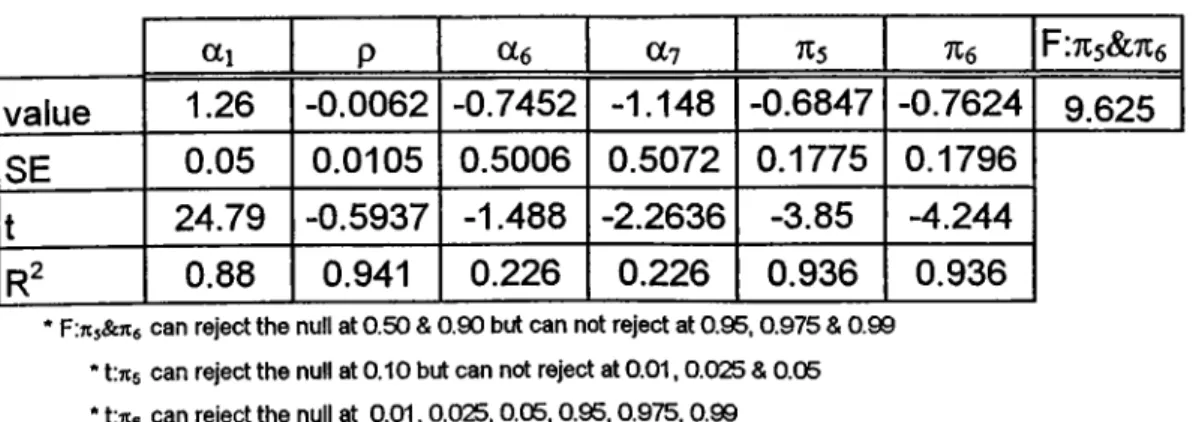
In this study, I tried to analyze and show the seasonal cointegration and error correction relations o f ISE, E, P, M l, M2, A and R for monthly data. First o f aU, by using HEGY (1990) and Franses (1991), I tried to drive all seasonal cointegration and error correction formulas for monthly data. In shortly, I drived the formulas for yi,t-i, y 2,n, y3,n, y3,t-2 , y4,t-i, y4,t-2, y5.t-i, y6,t-2, y6,t-i, y6,t-2, y 7,t-i, y 7.i-2, ys.t , Variables that are used to test significance o f the frequencies, then by running regression on:

(p*(B)y8,t = Ttiyi.t-l + Tt

2

y

2

,t

-1

+ 7t3y3,t-l + ît4y3,l-2+ Tt5y4,t-1 + Tt6y4,t-2 + 7t7y5,t-l + Tt

8

y

6

,t

-2

+ îtçyg,!-! + 7tloy6,t-2·*· ttliy7,t-l Ttl2y7,t-2 Pt + 6t

where (it can be seasonal dummies, and/or trend, and/or constant, or nothing.

I tried to test the significance o f the frequencies. The critical values are taken from Franses (1991). According to this regression results:

ISE, with constant and seasonal dummies and without lag, can not reject frequencies at Tti, tc2, Tt4,

ns,

tts, Jtio, 7ti2 , with the values -0.870, -2.170, -3.070, -2.810, 0.005, -2.500 and -0.919, accordingly. M oreover, 713, and

ne

are significant at 10% level.

2.310, -3.270 and -2.770. By using the F-test, it shows that only the 715, and Tie can not reject the null hypothesis, with the value 4.810.

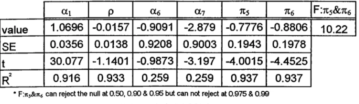
If I include trend in addition to constant and seasonal dummies, frequencies can not reject null at 712, Tig, tiio. Tin , with the values -2.300, -2.050, -2.850, -1.830, accordingly.

Moreover, TI3, , Tie, TI7 are significant at 10% level, with values, -1.840 and -3.060, 0.090,

Til, 714, Tie, TI9, and Tin are significant at 5% level, with values, —3.520, -3.580, -3.430,

-3.260, and -1.950. By using the F-test, it shows that all the coefficients reject the null

hypothesis.

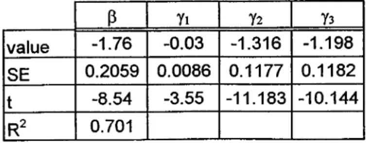
ISE, with constant and seasonal dummies and with 12 lags, can reject the null hypothesis at frequency at TI7 with the value -1.660, accordingly. M oreover, TI7 are significant at 5% level. By using the F-test, it shows that only the TI3, ... Tin can reject the null hypothesis, with the value 5.370.

I f I include trend to constant and seasonal dmiunies, still frequency that can not reject null is TI7 with the value -0.970, accordingly. M oreover, TI7 is significant at 5% level. By using the F-test, it shows that only the TI3, ... TI12can reject the null hypothesis, with the

value 5.660. Y ou can also see these results from Table 8.

with values, -2.030 and -3.130,

719

, and Tin are significant at 5% level, with values,