A comparative study of two-dimensional modeling methods for electromagnetic scattering data

(1)

A COMPARATIVE STUDY OF TWO-DIMENSIONAL

MODELING METHODS FOR ELECTROMAGNETIC

SCATTERING DATA

a thesis

submitted to the department of electrical and

electronics engineering

and the institute of engineering and science

of bilkent university

in partial fulfillment of the requirements

for the degree of

master of science

By

Anirudh S. Srinivasan

September 2007

(2)

Prof. Dr. Levent G¨urel (Supervisor)

I certify that I have read this thesis and that in my opinion it is fully adequate, in scope and in quality, as a thesis for the degree of Master of Science.

Prof. Dr. Ergin Atalar

I certify that I have read this thesis and that in my opinion it is fully adequate, in scope and in quality, as a thesis for the degree of Master of Science.

Prof. Dr. G¨ulbin Dural

Approved for the Institute of Engineering and Science:

Prof. Dr. Mehmet Baray

Director of the Institute Engineering and Science ii

(3)

To my parents, for always being there for me...

(4)

MODELING METHODS FOR ELECTROMAGNETIC

SCATTERING DATA

Anirudh S. Srinivasan

M.S. in Electrical and Electronics Engineering Supervisor: Prof. Dr. Levent G¨urel

September 2007

The aim of this research is to model two-dimensional data encountered in elec-tromagnetic scattering problems using model-based parameter estimation tech-niques. Once a highly accurate model is constructed from a few samples, the model can then be used to interpolate between or extrapolate from the original samples at any desired point and any number of times, thus reducing the amount of data needed to be stored in memory or required to be measured. An added advantage is that the computations required to be carried out on the numerical samples can instead be carried out on the analytical model, which may reduce the computational complexity.

It is intuitive that a higher number of terms in the model, increases the accu-racy, but additionally it has the unwanted effect of increasing the computational complexity and memory requirement as well. An additional goal, therefore, is to solve the optimization problem of obtaining a model by maximizing the accuracy and minimizing the number of terms.

Several modeling techniques are compared in this study, especially those based on matrix pencil methods. Some techniques for optimizing their performance have also been suggested. The pros and cons of each method are also discussed. It is shown that using the suggested techniques provides us with better models, but some pointers are also provided towards investigating more viable alternatives.

Keywords: Matrix pencil method (MPM), matrix enhancement and matrix pencil (MEMP) method, 2D modeling, electromagnetic scattering data.

(5)

¨

OZET

ELEKTROMANYET˙IK SAC

¸ ILIM VER˙ILER˙IN˙IN

˙IK˙I-BOYUTLU MODELLEME Y ¨ONTEMLER˙I ˙IC¸˙IN

KARS¸ILAS¸TIRMALI B˙IR C

¸ ALIS¸MA

Anirudh S. Srinivasan

Elektrik ve Elektronik Mühendisli˘gi, Yüksek Lisans Tez Yöneticisi: Prof. Dr. Levent Gürel

Eyl¨ul 2007

Bu ara¸stırmanın amacı, elektromanyetik sa¸cılım problemlerinde kar¸sıla¸sılan iki boyutlu verilerin model tabanlı parametre tahmin tekni˜gi kullanarak modellen-mesidir. Birka¸c örnekten olduk¸ca do˜gru bir model olu¸sturulduktan sonra, bu model kullanılarak orijinal örnekler istenilen herhangi bir noktada ve istenilen sayıda interpolasyon veya extrapolasyon yapılabilir, bu da hafızada depolanması ve öl¸cülmesi gereken verilerin sayısının azaltılmasını sa˜glar. Bu yöntemin di˜ger bir avantajı ise, hesaplamaların numerik örnekler yerine analitik model üzerinde yapılabilmesidir; bu sayede hesaplamaların karma¸sıklı˜gı azaltılmı¸s olur.

Modeldeki terim sayısının yüksek olması, daha hassas ¸cözüm imkanı sa˜glasa da, hesaplamanın karma¸sıklı˜gını ve hafıza gereksinimini de arttırır. Bu sebepten dolayı, bu ara¸stırmanın di˜ger bir amacı ise optimizasyon problemini ¸cözerek, has-sasiyeti maksimize edip, aynı zamanda terim sayısını minimumda tutmaktır.

Bu ¸calı¸smada, özellikle matris kalem metodu olmak üzere bir ¸cok modelleme tekni˜gi kar¸sıla¸stırılmı¸stır. Bu tekniklerin performansının arttırılabilmesi i¸cin bazı teknikler önerilmi¸s, avantajları ve dezavantajları tartı¸sılmı¸stır. Ayrıca, önerilen tekniklerin kullanılmasının daha iyi modeller sa˜gladı˜gı gösterilmi¸s, fakat uygu-lanılabilirli˜gi daha yüksek alternatifler geli¸stirmeye yönelik bazı noktalara da de˜ginilmi¸stir.

Anahtar sözcükler : Matris kalem yöntemi, matris geli¸stirme ve matris kalem yöntemi, iki-boyutlu modelleme, elektromanyetik sa¸cılım verisi.

(6)

Many people have been a part of my graduate education as teachers, colleagues and friends. But the first and foremost person whom I wish to thank is my advisor, mentor and guru, Prof. Dr. Levent G¨urel. I am enormously indebted to him for his guidance, encouragement, kind support and above all, patience.

I thank Prof. Dr. Ergin Atalar for agreeing to be a member of the jury for my thesis defense. My sincere gratitude is due to him for instilling hope during difficult times.

My thanks are also due to Prof. Dr. G¨ulbin Dural, who agreed to be the external jury member.

Besides these scholars, Prof. Dr. Ayhan Altınta¸s’s constant encouragement was a source of inspiration at all times.

I am also grateful to my friends and colleagues in BiLCEM, the Bilkent

Com-putational Electromagnetics Research Center. Special thanks are due to ¨Ozg¨ur

Erg¨ul for providing the data and programs needed for my experiments, numerous times, without grumbling, even once. I am also thankful to Tahir Malas and Dr. Idesbald van den Bosch for their helpful suggestions during my studies. I should also thank Ferhat Yıldırım, Ali Rıza Bozbulut and Alp Manyas for their support from time to time.

Special thanks to Dr. Rizwan Akram for his encouragement and helpful sug-gestions while writing this thesis. I am thankful to Caroline Foster for proof-reading this thesis and also for her support. My thanks are also due to the Department Secretary Ms. Muruvet Parlakay for assisting me on several occa-sions.

I am eternally grateful to my family and friends for their limitless support, without which I would not have been able to come to this point.

(7)

List of Figures

2.1 Synthetic data example. . . 5

2.2 A typical scattering problem. . . 6

2.3 Sphere surface approximated by tessellating triangles. . . 9

2.4 Real data example: 0.25λ Eφ. . . 10

3.1 Working of MPM. . . 12

3.2 Schematic of two-dimensional MPM. . . 14

3.3 Modeling 0.25λ Eφ data using MPM: real and imaginary parts of the data, model and absolute error. . . 15

3.4 Modeling 0.25λ Eφ data using MPM: magnitude and phase of the data, model and absolute error. . . 16

3.5 Modeling 0.5λ Eφ data using MPM: real and imaginary parts of the data, model and absolute error. . . 17

3.6 Modeling 0.5λ Eφ data using MPM: magnitude and phase of the data, model and absolute error. . . 18

3.7 Schematic of MEMP. . . 20

3.8 Inconsistent and wrong pairing by MEMP. . . 21 ix

(10)

4.1 Cross-pairing complex exponentials obtained from MEMP to

over-come the pairing problem. . . 24

4.2 Modeling 0.25λ Eφdata by cross-pairing complex exponentials

ob-tained from MEMP. . . 25

4.3 Modeling 0.25λ Eθ data by cross-pairing complex exponentials

4.4 Modeling 0.5λ Eφ data by cross-pairing complex exponentials

4.6 Modeling 1λ Eφ data by cross-pairing complex exponentials

4.7 Modeling 1λ Eθ data by cross-pairing complex exponentials

4.8 Modeling 1.5λ Eφ data by cross-pairing complex exponentials

4.10 Highest frequency resolvable by MEMP for the first dimension at

different sampling rates, for a 2λ Eφ data. . . 34

4.11 Highest frequency resolvable by MEMP for the second dimension

at different sampling rates, for a 2λ Eφ data. . . 35

4.12 Schematic diagram: successive removal of the smallest residual

(11)

LIST OF FIGURES xi

4.13 Improvement provided by SRSRFP over cross-pairing for modeling

a 0.25λ Eφ data. . . 38

a 0.25λ Eθ data. . . 39

a 0.5λ Eφ data. . . 40

a 0.5λ Eθ data. . . 41

a 1λ Eφ data. . . 42

a 1λ Eθ data. . . 43

a 1.5λ Eφ data. . . 44

a 1.5λ Eθ data. . . 45

4.21 Using genetic algorithms to reduce the number of terms in the model. 47 4.22 Improvement provided by genetic algorithms over cross-pairing for

modeling a 0.25λ Eφ data. . . 49

4.23 Improvement provided by genetic algorithms over cross-pairing for

modeling a 0.25λ Eθ data. . . 50

(12)

modeling a 1λ Eφ data. . . 53

modeling a 1λ Eθ data. . . 54

(13)

Chapter 1 Introduction

In computational electromagnetics, finding faster and memory-efficient algo-rithms has always been a requirement for being able to solve large real-life prob-lems. Electromagnetic scattering problems are a class of frequently encountered problems requiring the constant need for improved algorithms to achieve the above-mentioned goals. This includes radar cross section (RCS) calculation of airborne, stealth, and military targets, especially in the design and optimiza-tion stages. Bigger and complex geometries are more complicated to solve, typi-cally involving millions of unknowns and requiring huge computational resources. Model-based parameter estimation (MBPE) is one technique which promises to reduce the complexity of the algorithms involved in the solution of such problems.

1.1 Model-Based Parameter Estimation in

Computational Electromagnetics

MBPE is an age-old technique with applications not just limited to electromag-netics, but in almost all disciplines of engineering and science. MBPE attempts to approximate the numerical samples of the given data by an analytical model, whose parameters may be estimated by various methods. A general idea about

(14)

MBPE can be obtained from [1]. The solution of scattering problems usually in-volves performing multiple computations on the samples of two-dimensional data, several times and requires to be stored in memory for this purpose. Replacing the samples of this data by an approximate analytical expression has the advantage of letting us interpolate between the samples or extrapolate from them at any desired sampling point and any number of times as required. Thus a fewer val-ues can be stored in memory and further samples can be obtained as and when required. Besides, it is generally less complex to perform computations on an analytical model rather than on the numerical samples. This is especially advan-tageous for design and optimization purposes. This explains the motivation for this thesis.

The first challenge is to come up with a model that is most appropriate for representing the data in question. The next challenge is to choose the most effective parameter estimation technique to calculate approximate values for the parameters involved in the model such that the error due to the model is as low as possible. Typically, the higher the number of terms in the model, the lower the error will be. But a model with higher complexity may be of little use in most applications. Hence a trade-off has to made between complexity and accuracy.

However, the advantages of successfully modeling two-dimensional data do not stop here. Any situation that requires storing two-dimensional data samples can make use of MBPE to compress the data. Similar applications can be found not just in other areas of computational electromagnetics such as radar imaging and array processing, but also in many related areas of computational science and engineering.

1.2 Contribution

This thesis does not pretend to provide a panacea for the research problem men-tioned in the previous section, but rather involves a detailed investigation of pos-sible methods to achieve the posited goal and their advantages and disadvantages.

(15)

CHAPTER 1. INTRODUCTION 3

Some techniques for optimizing their performance have also been proposed. In Chapter 2, an account of the types of data that we have used for our ex-periments is offered. Our investigation about using the matrix pencil method (MPM) for modelling two-dimensional (2-D) data is described in Chapter 3. An-other method called matrix enhancement and matrix pencil (MEMP) method is introduced and its advantages and shortcomings are outlined.

Some techniques to overcome these shortcomings are proposed in Chapter 4 and experimental results are used to show the extent of success of these tech-niques. It is shown that even though the suggested techniques provide models with low error levels, it is more advantageous to reduce the complexity of the re-sulting models. Two optimization techniques are suggested to achieve this goal. Experimental results are used to illustrate the improvement obtained using these techniques. Conclusions arrived at and possible directions of the research for the future are offered in Chapter 5.

(16)

Types of Data Used for Modeling

There are two distinct types of data on which our modeling efforts have been concentrated, which we shall call real and synthetic data. Since we will be refer-ring to such data in almost every section of this thesis, a brief explanation about them is provided in this chapter.

2.1 Synthetic Data

Synthetic data is the data that we create artificially to test the performance of the modeling method in question. To elaborate, once an analytical model is decided upon to be more likely to represent a given data, and a modeling method has been chosen to estimate the parameters of the analytical model, the estimation accuracy of the modeling method needs to be tested. An obvious method to do this is to artificially assign arbitrary, yet meaningful, values to the parameters of the analytical model and to create a synthetic data so that the estimates obtained from the modeling method can be checked against the original values given. In general, an arbitrary amount of Gaussian noise is added to this data to simulate real-life data better. Synthetic data also has the advantage of enabling a much better comparison of estimation accuracy between different parameter retrieval methods than real-life data, which may have many inherent problems

(17)

CHAPTER 2. TYPES OF DATA USED FOR MODELING 5

in addition to noise. Let us now consider the analytical model given below for a two-dimensional noiseless data.

x(m, n) =

I

X

i=1

Rie(α1im+j2πf1im)e(α2in+j2πf2in) (2.1)

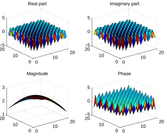
Equation (2.1) basically expresses the data samples as a weighted sum of I 2-D (damped) sinusoids at distinct 2-D frequencies. To illustrate creating synthetic data for testing purposes, Figure 2.1 shows the data created by using the

fol-lowing values for the parameters in Equation (2.1): I = 3; α1 = [0, 0, 0]; α2 =

[0, 0, 0]; f1 = [0.24, 0.24, 0.26]; f2 = [0.26, 0.24, 0.24]; 0 10 20 0 10 20 −5 0 5 Real part 0 10 20 0 10 20 −5 0 5 Imaginary part 0 10 20 0 10 201 2 3 Magnitude 0 10 20 0 10 20 −5 0 5 Phase

(18)

2.2 Real Data

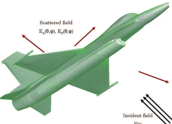
Although the synthetic data described in the previous section is useful for com-paring the performance of different parameter estimation methods and choosing the most accurate one, the actual usefulness of the investigated methods can only be demonstrated through their applicability for real-life data. The real-life data that we are interested in modeling is the electromagnetic scattering data from different shapes and sizes of scatterers—usually the far field components of the

electric-field, Eθ and Eφ which is a two dimensional data with directional

depen-dence on the θ and φ directions. A typical scattering problem is illustrated in Figure 2.2. It is to be noted here though, that when we refer to ‘real data,’ it means real-life data and not that the data is composed of real numbers. In fact real-life data is usually complex valued.

(19)

The usual approach in solving a scattering problem for an arbitrarily shaped geometry involves using integral equation techniques to solve for the unknown in-duced current on the object, in combination with the method of moments (MOM) to solve the resulting linear system. The electric-field integral equation (EFIE) for a perfectly conducting arbitrary surface can be written as

ˆt · ηT{J(r0_{)} = −ˆt · E}inc_(r) _(2.2)

where the operator T is given by

T{X(r0_{)} = ik} ½Z s dr0_{g(r, r}0_)X(r0_{) +} 1 k2 Z s dr0_{∇g(r, r}0_)∇0 _{· X(r}0₎ ¾ (2.3) and g(r, r0_{) =} eik|r−r 0_| 4π|r − r0_| (2.4)

is the Green’s function for the scalar Helmholtz equation. Similarly the magnetic-field integral equation (MFIE) can be written as

−Ωo

4πI{J(r

0_{)} + ˆ}_{n × K{J(r}0_{)} = −ˆ}_{n × H}inc_(r) _(2.5)

where the operator K is given by

K{X(r0_{)} =}

Z

s

dr0_{∇g(r, r}0_{) × X(r}0₎ _(2.6)

The combined-field integral equation (CFIE) is written as a linear combination of EFIE and MFIE,

CFIE = α(r)EFIE + [1 − α(r)]MFIE (2.7)

and is known to perform better than either EFIE or MFIE for certain problems [3]. J(r) in the above equations is the surface current density which is solved for using either EFIE, MFIE or CFIE and once known, the scattered electric and magnetic fields can be calculated from it.

Numerical solution of the above integral equations necessitates their dis-cretization, which is facilitated by the method of moments (MOM). MOM involves expanding the unknown current density using a set of known basis functions with

(20)

unknown coefficients. The solution of the resulting linear system provides the coefficient vector. The integral equations mentioned above can also be written as

L{f(x)} = g(x) (2.8)

where L is the linear operator of the equation, f(x) represents the unknown current distribution function, and g(x), the excitation given [3]. Method of moments involves expanding the unknown current distribution function in a series of known basis functions as follows.

f(x) ≈

N

X

n=1

an bn(x) (2.9)

where an is the coefficient for the nth basis function, bn(x). Since it is difficult in

most problems to obtain accurate values of an, the residual error defined by

R(x) = L ( _N X n=1 an bn(x) ) − g(x) (2.10)

is minimized to the extent possible. To facilitate this, another set of functions

tm(x) are used to weight both sides of (2.10) and tested for m = 1, 2, . . . , N as

Z dx tm(x) · N X n=1 an L{bn(x)} = Z dx tm(x) · g(x) (2.11)

Interchanging the order of summation and integration, a linear system is obtained as N X n=1 an Zmn = vm (2.12) where Zmn= Z dx tm· L{bn(x)} (2.13) and vm= Z dx tm(x) · g(x) (2.14)

Thus choosing appropriate and linearly independent basis functions results in N linearly independent equations for estimating N unknown coefficients. One of the most commonly used basis functions for electromagnetic problems is the Rao-Wilton-Glisson (RWG) function [7], which requires that the surface of the object

(21)

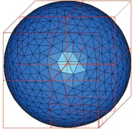
is discretized into small tessellating triangles, since the functions are defined on adjacent triangles. Figure 2.3 shows the surface of a sphere approximated by triangular meshing. Iterative algorithms are usually employed at this stage for solving this linear system efficiently and accurately. Techniques such as the fast

Figure 2.3: Sphere surface approximated by tessellating triangles.

multipole method (FMM) and its multi-level version MLFMA [2] are usually employed to accelerate the solution time and reduce memory requirements of the iterative solver. MLFMA proceeds to work by clustering the basis functions and clustering the clusters in a multi-level fashion and calculating the interactions between the basis and testing functions by performing operations at each level, such as aggregation, translation and disaggregation. A detailed explanation of MLFMA is beyond the scope of this thesis, but a good reference can be found in [3]. Clustering in MLFMA is accomplished by enclosing the geometry in a virtual cube and then recursively sub-dividing the cube into many levels of sub-cubes as shown in Figure 2.3. In other words, the cube enclosing the object is divided into 8 sub-cubes, each of which is sub-divided into 8 sub-cubes and so on until the

(22)

smallest sub-cube is of the size 0.25λ. The scattered field from portions of the object enclosed by sub-cubes of different sizes can be considered to constitute a set of scattering data from different sizes of scatterers.

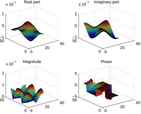
The procedures used for obtaining the results shown in this thesis involved modeling the scattered field components of the sub-cubes of a 16λ conducting sphere at a working frequency of 8 GHz. The sphere geometry was chosen because

the scattered field can be calculated analytically. The far-field components Eθ

and Eφ are functions of spherical directional co-ordinates θ and φ, as well as

frequency, but for our experimental purposes, only the directional variation at a specific frequency has been used as the two-dimensional input data.

A sample real data is shown in Figure 2.4 corresponding to the Eφcomponent

of a 0.25λ sub-cube of the above-mentioned 16λ sphere.

0 20 40 0 50 −1 0 1 x 10−7 Real part 0 20 40 0 50 −2 0 2 x 10−7 Imaginary part 0 20 40 0 500 1 2 x 10−7 Magnitude 0 20 40 0 50 −5 0 5 Phase

(23)

Chapter 3 Modeling Using Matrix Pencil

Methods

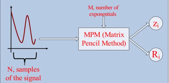
Many signals encountered in electromagnetics occur as solutions to differential or integral equations, describing the physics of the problem or those related analyti-cally to such signals. Since many of these solutions involve complex exponentials, they are a natural choice of basis functions for formulating an analytical model of the desired signal. Yıldırım in [8] dealt with describing one-dimensional sig-nals using the following model, which is basically a sum of weighted complex exponentials. y[k] = M X i=1 Ri eαik+j2πfik = M X i=1 Ri zik (3.1)

In the above equation, k is the sampling index, M is the number of

expo-nentials, Ri is the coefficient associated with the complex exponential zi. Once

the exponential set z is known, the equation becomes a simple linear system and the residuals can then be solved for, using the method of least squares among other possible methods. Among the methods available for estimating the complex

exponentials zi, the matrix pencil method (MPM) is said to be computationally

(24)

efficient and highly tolerant to noise [4]. Sarkar in [5] describes using MPM for estimating the parameters of a sum of weighted complex exponentials. For any two n-by-n matrices, A and B, the set of all matrices of the form A − λB with λ ∈ C, is said to be a pencil [6]. MPM attempts to construct a matrix pencil using the one dimensional data samples such that the generalized eigenvalues of the pencil becomes equivalent to the complex exponentials of (3.1). Thus given a set of one dimensional data samples, we can use MPM to obtain the complex

exponential set yi and then solve for the residuals Ri using the method of least

squares, thus obtaining an analytical model for the given samples.

Figure 3.1: Working of MPM.

Yıldırım, in his thesis [8] shows that MPM is a very effective and efficient tool for obtaining highly accurate models of one dimensional signals. It is therefore, understandably tempting, to try using MPM for modeling two dimensional data. This chapter describes our investigation in this direction.

3.1 Two-Dimensional Modeling Using MPM

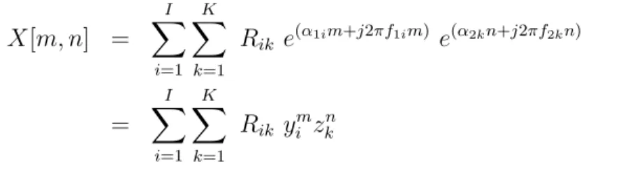
It is perhaps intuitive that if a one-dimensional signal requires one set of complex exponentials (poles) to construct a highly accurate model, a two-dimensional signal would require two such related sets. Thus Equation (3.1) can be modified

(25)

CHAPTER 3. MODELING USING MATRIX PENCIL METHODS 13

to incorporate another set of exponentials to describe the second dimension, as follows. X[m, n] = I X i=1 K X k=1 Rik e(α1im+j2πf1im) e(α2kn+j2πf2kn) = I X i=1 K X k=1 Rik yimzkn (3.2)

As before, m and n are the sampling indices in each direction. I is the

number of complex exponentials yi associated with the first dimension and K

is the number of exponentials zi for the second dimension. Rik are the weights

(coefficients) associated with each ‘pair’ of poles. Assuming that this equation would be able to accurately represent a given two-dimensional signal, the next step is to obtain the estimates of the parameters y and z.

A two-dimensional data matrix of size M × N is basically a set of M row vectors or a set of N column vectors, with each vector being an individual signal. As mentioned in the previous section, MPM can be employed to find the charac-teristic complex exponentials of such a one-dimensional signal. This means, for a given two-dimensional signal, we would be able to find M × N complex exponen-tial sets if one were to perform MPM on each row and each column. This would be a huge set of exponentials that would increase the complexity of the model. What is needed is just one set of exponentials corresponding to each dimension of the data.

One simple solution is to arbitrarily pick one set of exponentials obtained from one of the rows and another from one of the columns, thus being able to incorporate the characteristics of both dimensions of the data into the model and also retaining a lower level of complexity. Once y and z have been obtained, the residuals can be calculated using the method of least squares. It is to be noted here that if complexity could be tolerated, a brute force optimization could be done to select the best set of poles, y and z, that give the least error in modeling. Figure 3.2 shows a schematic of the method just described.

(26)

Figure 3.2: Schematic of two-dimensional MPM.

3.1.1 Results and Discussion

The following are the results of modeling the Eφ component of a 0.25 λ cube,

part of a 16 λ sphere data. The data is sampled with 41 points in φ and 21 points

in θ. MPM was used on the 40th _{row, corresponding to φ=351}◦_{, to obtain 10}

complex exponentials and on the 20th _{column, corresponding to θ=171}◦ _{to obtain}

20 poles. Figure 3.3 shows the real and imaginary parts of the original data,the obtained model and the absolute error. Figure 3.4 shows a similar plot for the magnitude and phase of the data, model and absolute error. It is obvious from these plots that the model obtained closely resembles the original signal. The error is about two orders of magnitude lower than the signal.

(27)

CHAPTER 3. MODELING USING MATRIX PENCIL METHODS 15 Figure 3.3: Mo deling 0.25 λ Eφ data using MPM: real and imaginary parts of the data, mo del and absolute error.

(28)

Figure 3.4: Mo deling 0.25 λ Eφ data using MPM: magnitude and phase of the data, mo del and absolute error.

(29)

CHAPTER 3. MODELING USING MATRIX PENCIL METHODS 17 Figure 3.5: Mo deling 0.5 λ Eφ data using MPM: real and imaginary parts of the data, mo del and absolute error.

(30)

Figure 3.6: Mo deling 0.5 λ Eφ data using MPM: magnitude and phase of the data, mo del and absolute error.

(31)

Although these plots show just the absolute error, the best way to judge the performance of a modeling method is using the relative error. For the above results, the relative error at the point of maximum absolute error was approxi-mately 1.3%. Figures 3.5 and 3.6 show similar plots for a 0.5λ cube data. As can be seen from the first set of results, we are able to obtain models with er-rors as low as nearly 1% using this modeling method. Another advantage of this modeling method is its simplicity and low computational cost.

However, the accuracy of the models obtained is still not sufficient for most applications. Even though we were able to obtain nearly 1% error for the first set of data, we were able to reach only 10% for the second set. Experiments were conducted on different sets of data, but in all cases, we were not able to obtain errors below the threshold of 1%. Using such models (even the 1% ones) might distort the accuracy of the parent algorithm. At the same time though, if loss in accuracy can be tolerated over the need for reducing memory requirements, this method might be suitable. Another disadvantage of this method is that we have limited control over the reduction of the error.

3.2 Two-Dimensional Modeling Using MEMP

The method described in the previous section attempts to obtain one set of com-plex exponentials describing the characteristics of the data in one dimension and another set corresponding to the other direction, but an approximation is made when we choose the exponentials obtained from only one row/column to model the rest of the data as well. As can be clearly seen from the results, this approx-imation affects the accuracy of the models obtained at the end.

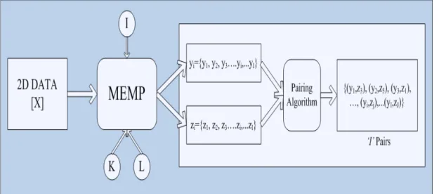
Yingbo Hua, in [9] describes a new method called the matrix enhancement and matrix pencil (MEMP) method to obtain two ‘related’ sets of complex ex-ponentials that could model the two-dimensional data as a whole. This method could possibly be called the two-dimensional extension to MPM.

(32)

Figure 3.7: Schematic of MEMP.

its generalized eigenvalues turn out to be the complex exponentials of Equation (3.1). For MEMP, the challenge is to construct two such matrix pencils, so that the generalized eigenvalues of each pencil would correspond to the complex exponential sets y and z respectively as in Equation (3.3).

X[m, n] = I X i=1 Ri eα1im+j2πf1im eα2in+j2πf2in = I X i=1 Ri yimzin (3.3)

It is to be noted here that the model that MEMP uses has equal number of exponentials for both dimensions, unlike the method described in the previous section. The ‘matrix enhancement and matrix pencil’ method is called so be-cause it attempts to enhance the rank condition of the given data matrix by a partitioning-and-stacking process before constructing the matrix pencils. This is done to increase the efficiency and accuracy of estimation of the two sets of com-plex exponentials. These poles can be obtained from the principal eigenvectors of the enhanced matrix by the construction of two related matrix pencils. The following schematic in Figure 3.7 describes this method visually.

(33)

3.2.1 The ‘Pairing’ Problem

The keyword here though, is to obtain two ‘related’ sets of complex exponentials.

What this means is that, there is a one to one correlation between yi and zi

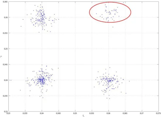
according to the model and that it is not just enough to obtain the two sets of poles, but it is also equally important to know the correlation between them. The MEMP method obtains the complex exponentials corresponding to each dimension separately and then attempts to use a ‘pairing’ technique to relate the two together. However, this pairing technique does not always provide us with the correct and reliable pairs, especially in the case of noisy data or real time data. This, as we shall see, poses the biggest challenge in using the MEMP method directly to find the parameters of our model. To illustrate this, let us consider the synthetic data shown in Figure 2.1, constructed using the model in Equation (2.1) with the same parameters. White gaussian noise of SNR = 20 dB is added to this data and MEMP is used to estimate the poles.

(34)

Figure 3.8 shows 200 independent estimates for the three 2-D frequencies for K = 10; L = 10. As can be seen, MEMP manages to estimate the poles to a reasonable level of accuracy, but ends up with a wrong pair (0.26,0.26) several times.

This inconsistent pairing manifests in very high error levels (as much as 100%) when MEMP is applied for modeling real data. Some methods and techniques that we have investigated towards overcoming this problem are discussed in Chap-ter 4.

3.3 Two-Dimensional Modeling Using Methods

Similar to MEMP

The pairing problem encountered by MEMP is well documented in the literature. We investigated a few other 2-D harmonic retrieval methods that purportedly overcome this pairing problem, but we realized that all those methods apply only for synthetic data.

The modified MEMP [12]–[13] method by Chen, et al., attempts to construct the second matrix pencil using the generalized eigenvectors from the first matrix pencil, such that the generalized eigenvalues obtained, turn out to be in the correct paired order with respect to the first set of poles. This method works perfectly well for artificial data, but fails miserably for real data.

The 2-D ESPRIT method [14]–[15], the algebraically coupled matrix pencils (ACMP) algorithm [16], the diagonal matrix pencil (DMP) method [17] are a few other methods similar to MEMP that either attempt to overcome the pairing problem or use similar techniques to estimate the complex exponentials. However, just like the modified MEMP method, these methods fail for real data, even if their performance for artificial data is good. Without showing any results at this point, we shall just state here that the MEMP method provides a better quality of estimates than these other methods.

(35)

Chapter 4 Optimizing the MEMP Method

In the previous chapter, we saw that the MEMP method and other similar meth-ods for two-dimensional harmonic retrieval suffer from the ‘pairing’ problem. Even though some alternative pairing methods in the literature work perfectly for artificial data, they fail for real data, especially the scattering data that we would like to model. In this chapter, we discuss methods that we have investigated for overcoming this pairing problem and thus enabling us to use this method for our modeling purposes.

4.1 Cross-Pairing

One obvious way to overcome the pairing problem is to ‘cross’ the two sets of complex exponentials, so that we obtain a set of all possible combinations of the exponential sets, as described in Figure 3.1. In other words, we cross I sets of y’s

and z’s obtained from MEMP to acquire I2 _{pairs, which will include the ‘best’}

exponential pairs, i.e., the ones that characterize the data as closely as possible.

However, we now have to calculate I2 _{residuals using the method of least squares.}

It is worth noting here that cross-pairing is basically similar to modifying our model as in Equation (3.3) into Equation (3.2), with K being equal to I this

(36)

CROSSING {[(y1,z1), (y1,z2), (y1,z3), …, (y1,zi), … (y1,zI)], [(y2,z1), (y2,z2), (y2,z3), …, (y2,zi), … (y2,zI)] ……… ………... [(yi,z1), (yi,z2), (yi,z3), …, (yi,zi), … (yi,zI)] ……….. ……….. [(yI,z1), (yI,z2), (yI,z3), …, (yI,zi), … (yI,zI)]} y1 y2 y3 . . . yi . . . yI z1 z2 z3 . . . zi . . . zI ‘I2’ Pairs

Complex Exponentials from MEMP

Figure 4.1: Cross-pairing complex exponentials obtained from MEMP to over-come the pairing problem.

time. Instead of a single summation, we now have a double summation making sure that each and every y is paired with each and every z.

Figure 4.2 shows the results of modeling by cross pairing the MEMP

exponen-tials on a 0.25λ Eφ data sampled with 41 points in φ and 21 points in θ direction.

As can be clearly seen, the error decreases gradually as we increase the number

of terms, I. Figure 4.3 shows a similar result for the Eθ component. The size of

the scatterer, that is, the size of the sub-cubes from which the scattered data is obtained is gradually increased from Figures 4.4 to 4.9.

The advantage of such a technique is clearly obvious in the results shown below. Until this point we had utmost 1% relative error for even simple data, but as can be seen in the following plots, we can now reach error levels as low as

10−6 _{(relative) in some cases. The second advantage is that we now have control}

over the error levels. In other words, if 0.1% error is sufficient for a particular application, we can limit the number of complex exponentials used in the model thereby reducing its complexity.

(37)

CHAPTER 4. OPTIMIZING THE MEMP METHOD 25 0 5 10 15 20 25 10 −14 10 −12 10 −10 10 −8 10 −6 I

Max. Abs. Error (MAE)

0 5 10 15 20 25 10 −5 10 −4 10 −3 10 −2 10 −1 10 0 I

Relative Error at point of occurance of MAE

0 5 10 15 20 25 10 −8 10 −6 10 −4 10 −2 10 0 I MAE/norm(Data) 0 5 10 15 20 25 10 −6 10 −4 10 −2 10 0 I Norm(Error)/Norm(Data) Figure 4.2: Mo deling 0.25 λ Eφ data by cross-pairing complex exp onen tials obtained from MEMP .

(38)

0 100 200 300 400 500 600 700 10 −14 10 −12 10 −10 10 −8 10 −6 I

0 100 200 300 400 500 600 700 10 −6 10 −4 10 −2 10 0 10 2 I

0 100 200 300 400 500 600 700 10 −8 10 −6 10 −4 10 −2 10 0 I MAE/norm(Data) 0 100 200 300 400 500 600 700 10 −6 10 −5 10 −4 10 −3 10 −2 10 −1 10 0 I Norm(Error)/Norm(Data) Figure 4.3: Mo deling 0.25 λ Eθ data by cross-pairing complex exp onen tials obtained from MEMP .

(39)

CHAPTER 4. OPTIMIZING THE MEMP METHOD 27 0 5 10 15 20 25 10 −11 10 −10 10 −9 10 −8 10 −7 10 −6 I

0 5 10 15 20 25 10 −4 10 −3 10 −2 10 −1 10 0 10 1 I

0 5 10 15 20 25 10 −6 10 −5 10 −4 10 −3 10 −2 10 −1 I MAE/norm(Data) 0 5 10 15 20 25 10 −5 10 −4 10 −3 10 −2 10 −1 10 0 I Norm(Error)/Norm(Data) Figure 4.4: Mo deling 0.5 λ Eφ data by cross-pairing complex exp onen tials obtained from MEMP .

(40)

0 200 400 600 800 10 −11 10 −10 10 −9 10 −8 10 −7 10 −6 I

0 100 200 300 400 500 600 700 10 −4 10 −3 10 −2 10 −1 10 0 10 1 I

0 200 400 600 800 10 −6 10 −5 10 −4 10 −3 10 −2 10 −1 I MAE/norm(Data) 0 100 200 300 400 500 600 700 10 −5 10 −4 10 −3 10 −2 10 −1 10 0 I Norm(Error)/Norm(Data) Figure 4.5: Mo deling 0.5 λ Eθ data by cross-pairing complex exp onen tials obtained from MEMP .

(41)

CHAPTER 4. OPTIMIZING THE MEMP METHOD 29 0 5 10 15 20 25 10 −10 10 −9 10 −8 10 −7 10 −6 I

0 5 10 15 20 25 10 −3 10 −2 10 −1 10 0 10 1 I

0 5 10 15 20 25 10 −5 10 −4 10 −3 10 −2 10 −1 I MAE/norm(Data) 0 5 10 15 20 25 10 −4 10 −3 10 −2 10 −1 10 0 I Norm(Error)/Norm(Data) Figure 4.6: Mo deling 1λ Eφ data by cross-pairing complex exp onen tials obtained from MEMP .

(42)

0 100 200 300 400 500 600 700 10 −10 10 −9 10 −8 10 −7 10 −6 I

0 100 200 300 400 500 600 700 10 −3 10 −2 10 −1 10 0 10 1 I

0 100 200 300 400 500 600 700 10 −5 10 −4 10 −3 10 −2 10 −1 I MAE/norm(Data) 0 100 200 300 400 500 600 700 10 −4 10 −3 10 −2 10 −1 10 0 I Norm(Error)/Norm(Data) Figure 4.7: Mo deling 1λ Eθ data by cross-pairing complex exp onen tials obtained from MEMP .

(43)

CHAPTER 4. OPTIMIZING THE MEMP METHOD 31 0 100 200 300 400 500 600 700 10 −9 10 −8 10 −7 10 −6 I 2

0 100 200 300 400 500 600 700 10 −2 10 −1 10 0 10 1 I 2

0 100 200 300 400 500 600 700 10 −4 10 −3 10 −2 10 −1 I 2 MAE/norm(Data) 0 100 200 300 400 500 600 700 10 −2 10 −1 10 0 I 2 Norm(Error)/Norm(Data) Figure 4.8: Mo deling 1.5 λ Eφ data by cross-pairing complex exp onen tials obtained from MEMP .

(44)

0 100 200 300 400 500 600 700 10 −9 10 −8 10 −7 10 −6 I

0 100 200 300 400 500 600 700 10 −2 10 −1 10 0 10 1 I

0 100 200 300 400 500 600 700 10 −4 10 −3 10 −2 10 −1 I MAE/norm(Data) 0 100 200 300 400 500 600 700 10 −3 10 −2 10 −1 10 0 I Norm(Error)/Norm(Data) Figure 4.9: Mo deling 1.5 λ Eθ data by cross-pairing complex exp onen tials obtained from MEMP .

(45)

CHAPTER 4. OPTIMIZING THE MEMP METHOD 33

As obvious as the advantages of this technique were, the disadvantage is also apparent. We now have a much greater number of terms in the model than in previous cases. Crossing 10 complex exponentials from each dimension leads us to

100 terms in the final model. Therefore the complexity grows with I2 _{instead of}

I. This liability in some ways overshadows the other advantages since it may not be worthwhile to apply this model in some applications. The following sections describe a couple of optimization techniques that we have investigated to reduce number of terms in these low error models.

Another problem that we have encountered is that, as the complexity of the data becomes higher, that is, as we try to model the scattering data from bigger sub-cubes, it gets more and more difficult to model. As can be seen from the plots above, to reach a particular relative error level for a 1.5λ data, we need many more terms in the model when compared to a 0.25λ data. For increasing the applicability of these modeling techniques, solving this problem would open many doors. But this is beyond the scope of this thesis and is left as future work. Before we can have a look at the optimization techniques, let us have a brief look at the effect of sampling.

4.2 Effect of Sampling

An important point to consider at this juncture is the sampling rate at which the data that we would like to model is sampled. We have to ensure that the sampling rate is sufficient enough for MEMP to be able to resolve all available frequency components. If the sampling is insufficient to resolve even one or two frequency components, then the error would be very high even with cross-pairing and that cannot be brought down.

For the real data used in the experiments mentioned in this thesis, since there is no prior information on all the exact frequency components available in the data, as would be the case for most real data, we have come up with a method to determine if the sampling is enough for MEMP or not. Figure 4.10 shows the

(46)

highest frequency corresponding to one of the dimensions, resolved by MEMP for the same data sampled at different rates. Basically what we have done here is to plot the damped signal corresponding to the highest frequency term in the model

without considering the residuals. The data is the Eφ component of a 2λ cube

data and the sampling with 161 φ points and 81 θ points is considered as the reference data. As is easily understandable from the figure, for the higher sam-pling rates, MEMP resolves the highest frequency present in the reference data as well, but for lower sampling rates it is not able to resolve those components. If we use such lower sampling rates and expect MEMP and cross-pairing to provide us with good models, then we are bound to be disappointed. Figure 4.11 shows a similar figure for the frequencies corresponding to the second dimension of the data and the same conclusions can be drawn for this case too.

0 50 100 150 200 250 300 350 400 −1.5 −1 −0.5 0 0.5 1 1.5 φ° ∆_s=1; 161x81 ∆_s=2; 81x41 ∆_s=4; 41x21 ∆_s=8; 21x11 ∆_s=16; 11x6

Figure 4.10: Highest frequency resolvable by MEMP for the first dimension at

(47)

CHAPTER 4. OPTIMIZING THE MEMP METHOD 35 0 20 40 60 80 100 120 140 160 180 −1 −0.8 −0.6 −0.4 −0.2 0 0.2 0.4 0.6 0.8 1 θ° ∆_s=1; 161x81 ∆_s=2; 81x41 ∆_s=4; 41x21 ∆_s=8; 21x11 ∆_s=16; 11x6

Figure 4.11: Highest frequency resolvable by MEMP for the second dimension at

different sampling rates, for a 2λ Eφ data.

4.3 Methods for Reducing the Number of

Terms

As mentioned in Section 4.1, cross-pairing helps us obtain models with very low error levels, but increases the complexity of the model due to the huge number of terms involved. Common sense dictates that, after cross-pairing, there would be many unnecessary frequencies in the model which would have little or no effect at all. The complexity of the model can be vastly reduced by removing these complex exponentials with very limited compromise on the error levels. Besides, we can obtain a better control over the trade-off between complexity and accuracy of the models.

Two techniques that we have investigated to achieve this above-mentioned goal are described in the following sections.

(48)

4.3.1 Successive Removal of the Smallest Residual

Frequency Pair

While obtaining the residuals for the cross-paired complex exponentials, the method of least squares gives us a very good indication as to which frequencies are more important to the model and which frequencies are not, by intelligently allotting higher weights to those frequencies which have a more important con-tribution towards the model and lower weights to unnecessary terms.

Figure 4.12: Schematic diagram: successive removal of the smallest residual fre-quency pair (SRSRFP).

(49)

This makes it easier to filter out those frequencies which have limited con-tribution to the model. Therefore an intuitive method to reduce the number of terms in the model obtained after cross-pairing would be to simply remove those complex exponentials associated with the smallest residuals. We have developed a simple iterative algorithm to implement this idea as described below.

To illustrate the problem in hand, let us assume that we have a model with I2

pairs by cross-pairing I number of complex exponentials obtained from MEMP.

The goal now is to reduce the number of poles from I2 _{to a lower value such}

that the accuracy is not affected too much. The first step is to sort the I2

residuals in the descending order and start removing the poles associated with the residuals at the bottom of the list, one by one. Each time we remove a pole the values of the other residuals should be re-calculated so as to distribute the weights between the available frequencies. The error due to the new model should also be evaluated at each step. This procedure is carried out iteratively until a satisfactory compromise has been obtained between the number of terms and the error level. We now have a better control over the model’s accuracy and complexity, meaning that we can use as smaller a number of exponentials as is necessary for a desired accuracy.

4.3.2 Results and Discussion

As can be seen from the plots below, this method helps us obtain low-error models with a much lower number of terms, compared to cross-pairing. Another way to look at the results is that for the same level of accuracy as obtained with cross-pairing, we can now use lesser number of complex exponentials. For example, in Figure 4.13, the error obtained with 625 terms using cross-pairing can now be obtained with less than half of that number, after removing the terms with the smallest residuals. Similar improvements can be seen in the other plots as well, each corresponding to a slightly bigger size of the scatterer. Although this seems like a very reasonable improvement, further improvement is usually desirable for most applications. Thus we have resorted to a more scientific optimization technique as described in the next section.

(50)

Figure 4.13: Impro vemen t pro vided by SRSRFP ov er cross-pairing for mo deling a 0.25 λ Eφ data.

(51)

CHAPTER 4. OPTIMIZING THE MEMP METHOD 39 Figure 4.14: Impro vemen t pro vided by SRSRFP ov er cross-pairing for mo deling a 0.25 λ Eθ data.

(52)

(53)

(54)

Figure 4.17: Impro vemen t pro vided by SRSRFP ov er cross-pairing for mo deling a 1λ Eφ data.

(55)

CHAPTER 4. OPTIMIZING THE MEMP METHOD 43 Figure 4.18: Impro vemen t pro vided by SRSRFP ov er cross-pairing for mo deling a 1λ Eθ data.

(56)

(57)

(58)

4.3.3 Genetic Algorithms

As can be gathered from the previous sections, we have an optimization problem at hand. Cross-pairing results in a huge pool of complex exponential pairs from which we can pick a limited number to provide us with a model with a desired accuracy. In other words, we have to minimize the number of terms required in the model, while maximizing the accuracy that can be obtained with a particular number of terms. We have resorted to genetic algorithms to resolve this issue.

A genetic algorithm is a global optimization technique inspired by the field of evolutionary biology to find exact or approximate solutions to search and opti-mization problems in computational sciences [18]. It is a sophisticated optimiza-tion technique which optimizes a funcoptimiza-tion to a specified criterion and is widely used in many science and engineering problems. It is implemented as a computer simulation where candidate solutions to a given optimization problem are ab-stractly treated as citizens in a generation who evolve towards better solutions in each successive generation. The worthiness of each citizen is evaluated by a cost function which tries to find the citizen with the optimal cost. The characteristics of the citizens are modified in each successive generation by algorithms inspired by evolutionary biology concepts such as mutation, inheritance, crossover etc. The algorithm is expected to have found an optimal solution when it converges, i.e., there is little or no improvement in cost for several successive generations. It may also be prematurely terminated when a desired cost is achieved or when the maximum number of generations has been reached. More information on genetic algorithms can be obtained from [18].

For our application, the objective is to select the best iy number of complex

exponential pairs from ix = I2 _{pairs resulting from cross-pairing. The total}

number of ways in which, iy objects can be chosen from ix objects is given by

the combination function, ixC_{iy, which gives the total number of combinations of}

pairs possible. This is a very huge number as illustrated below. If we obtain 25 pairs from MEMP, obtain 625 pairs by cross-pairing them and need to select 50

pairs from this 625, we could possibly obtain 625C_{50 which is nearly 10}74_possible

(59)

Figure 4.21: Using genetic algorithms to reduce the number of terms in the model.

to our problem and hence is a citizen of the general population which includes all such possible sets. The cost function ascertains which of these sets are worth more, by evaluating the error due to the model obtained by using the said set of pairs. The best citizen at the end of the simulation is the one which provides the least error possible with 50 pairs.

The parameters controlling the accuracy and performance of such a simulation include the following. Pool size (ps) specifies a subset of the general population to initialize the algorithm. Mutation rate (mr) specifies the rate at which mutation occurs from one generation to the other. Maximum number of generations (igen) until which the simulation is to be run is another required parameter. Certain other parameters have been set to constant default values for all our simulations.

4.3.4 Results with Genetic Algorithms

Figures 4.22 to 4.29 illustrate the improvement provided by using genetic algo-rithms for our modeling purposes. The number of terms in the model has now been reduced significantly compared to the models obtained after cross-pairing.

(60)

The reduction is much more significant than those provided by the method de-scribed in Section 4.3.1. For example, let us consider the case of a 0.25λ cube

data’s Eφ component as shown in Figure 4.22. The minimum error obtained

by cross-pairing 25 MEMP pairs, i.e., 625 terms can now be obtained with only 200 terms. Thus we have a less complex model providing a low error level. If a compromise on the accuracy can be tolerated, we can use a still lesser number of terms in the model. Basically, this means that we have very good control over the trade-off between complexity and accuracy. Results obtained from different sizes of scatterers are shown in Figures 4.23 to 4.29 with the size of the scatterer being increased gradually. It can be clearly seen that genetic algorithms provide significant improvement from cross-pairing for all the cases.

However, this method is not without its disadvantages either. The price we have to pay to obtain such low error models with less complex models is the increase in computational complexity. The cost function which incorporates a least squares routine to evaluate the modeling error is called for each member of the specified pool and for each generation of citizens. Thus the complexity of using genetic algorithms increases with the product of the pool size and the number of generations. This is counter-effective because higher number of generations is required to reach convergence or at least lower levels of errors. Higher number of citizens in the pool also signifies a better chance of convergence. Nevertheless, if an application requires a low error model to be used over and over again and can tolerate a one-time complexity in the modeling phase, this method can prove to be very useful.

(61)

CHAPTER 4. OPTIMIZING THE MEMP METHOD 49 0 100 200 300 400 500 600 700 10 −12 10 −10 10 −8 10 −6 I

0 100 200 300 400 500 600 700 10 −6 10 −4 10 −2 10 0 10 2 I

0 100 200 300 400 500 600 700 10 −8 10 −6 10 −4 10 −2 10 0 I MAE/norm(Data) 0 100 200 300 400 500 600 700 10 −6 10 −4 10 −2 10 0 I Norm(Error)/Norm(Data)

Cross−pairing Genetic Algorithms

Figure 4.22: Impro vemen t pro vided by genetic algorithms ov er cross-pairing for mo deling a 0.25 λ Eφ data.

(62)

0 100 200 300 400 500 600 700 10 −14 10 −12 10 −10 10 −8 10 −6 I

0 100 200 300 400 500 600 700 10 −6 10 −4 10 −2 10 0 10 2 I

0 100 200 300 400 500 600 700 10 −8 10 −6 10 −4 10 −2 10 0 I MAE/norm(Data) 0 100 200 300 400 500 600 700 10 −6 10 −5 10 −4 10 −3 10 −2 10 −1 10 0 I Norm(Error)/Norm(Data)

Figure 4.23: Impro vemen t pro vided by genetic algorithms ov er cross-pairing for mo deling a 0.25 λ Eθ data.

(63)

CHAPTER 4. OPTIMIZING THE MEMP METHOD 51 0 100 200 300 400 500 600 700 10 −11 10 −10 10 −9 10 −8 10 −7 10 −6 I

0 100 200 300 400 500 600 700 10 −4 10 −3 10 −2 10 −1 10 0 10 1 I

0 100 200 300 400 500 600 700 10 −6 10 −5 10 −4 10 −3 10 −2 10 −1 I MAE/norm(Data) 0 100 200 300 400 500 600 700 10 −5 10 −4 10 −3 10 −2 10 −1 10 0 I Norm(Error)/Norm(Data)

Figure 4.24: Impro vemen t pro vided by genetic algorithms ov er cross-pairing for mo deling a 0.5 λ Eφ data.

(64)

0 100 200 300 400 500 600 700 10 −11 10 −10 10 −9 10 −8 10 −7 10 −6 I

0 100 200 300 400 500 600 700 10 −4 10 −3 10 −2 10 −1 10 0 10 1 I

0 100 200 300 400 500 600 700 10 −6 10 −5 10 −4 10 −3 10 −2 10 −1 I MAE/norm(Data) 0 100 200 300 400 500 600 700 10 −5 10 −4 10 −3 10 −2 10 −1 10 0 I Norm(Error)/Norm(Data)

(65)

CHAPTER 4. OPTIMIZING THE MEMP METHOD 53 Figure 4.26: Impro vemen t pro vided by genetic algorithms ov er cross-pairing for mo deling a 1λ Eφ data.

(66)

0 100 200 300 400 500 600 700 10 −10 10 −9 10 −8 10 −7 10 −6 I

0 100 200 300 400 500 600 700 10 −3 10 −2 10 −1 10 0 10 1 I

0 100 200 300 400 500 600 700 10 −5 10 −4 10 −3 10 −2 10 −1 I MAE/norm(Data) 0 100 200 300 400 500 600 700 10 −4 10 −3 10 −2 10 −1 10 0 I Norm(Error)/Norm(Data)

Figure 4.27: Impro vemen t pro vided by genetic algorithms ov er cross-pairing for mo deling a 1λ Eθ data.

(67)

CHAPTER 4. OPTIMIZING THE MEMP METHOD 55 Figure 4.28: Impro vemen t pro vided by genetic algorithms ov er cross-pairing for mo deling a 1.5 λ Eφ data.

(68)

(69)

Chapter 5 Conclusion and Future Work

In this thesis, we have presented a couple of methods to model two-dimensional electromagnetic scattering data and proposed some techniques to improve the effi-ciency of these methods. In Chapter 2, we have introduced the types of data that we have used for our experimental purposes. Synthetic data has been used for benchmarking the effectiveness of the two-dimensional harmonic retrieval meth-ods available in the literature. We have used real data to evaluate and compare the performance of the various methods presented in the rest of the chapters. The way we obtain both these types of data has been explained.

The matrix pencil method has been introduced in Chapter 3 and its applica-tion to one-dimensional modeling has been explained. We have proposed a new method to apply MPM for two-dimensional modeling purposes. The pros and cons of such a technique have been discussed. The matrix enhancement and ma-trix pencil method has been introduced as an alternative to solve the problems experienced with using MPM for two-dimensional modeling. The ‘pairing’ prob-lem of the MEMP method has been explained as a bottleneck stopping us from being able to use it effectively. A note on a few other similar two-dimensional harmonic retrieval methods has been provided. In Chapter 4, we have proposed new methods and techniques to overcome the bottleneck mentioned in the pre-vious paragraph. We have proposed cross-pairing to overcome MEMP’s pairing problem. We have also shown that we are able to obtain low-error models using

(70)

cross-pairing using experimental results. The pros and cons of this technique have been discussed and the need for reducing the complexity of the model has been mentioned. A short note on the effect of sampling has been provided. Two tech-niques have been proposed to reduce the number of terms in the model obtained with cross-pairing.

Successive removal of the smallest residual frequency pair has been proposed as a method to retain the low error models provided by cross-pairing, but with a much smaller number of terms in the final model, thus reducing its complexity while retaining the accuracy. Experimental results have been provided and the effectiveness and shortcomings of this method have been discussed. Genetic algo-rithms have been introduced as an effective optimization technique to minimize the complexity of the models while maximizing the accuracy to the extent possi-ble. The details of such an implementation have been provided and the price to be paid for its advantages has been discussed. The improvement obtained using genetic algorithms from the results of cross-pairing has been illustrated clearly using experimental results.

Although we have proposed effective modeling techniques, some additional work is required for improving the efficacy of these methods before applying for real-life problems. More viable alternatives may be possible and need to be researched. One possible future direction of research could be to change the basis functions used in the model. All the methods investigated in this thesis involved using complex exponentials as the basis functions. Although the validity of this choice has been described in Chapter 3, using different basis functions such as spherical harmonics might prove to be a more appropriate choice, especially for scattering data.

To sum up, in this thesis we have provided an insight into modeling two-dimensional electromagnetic scattering data especially using methods based on the matrix pencil method. The advantages of various methods, bottlenecks en-countered, ways to overcome such problems, techniques to optimize their perfor-mance and their applicability have been discussed in detail. This thesis should provide a substantial basis for future directions of research to obtain more viable

(71)

CHAPTER 5. CONCLUSION AND FUTURE WORK 59

modeling techniques or, improve the methods discussed so as to apply them to real life problems.

(72)

[1] Edmund K. Miller, “Model-based parameter estimation in electro-magnetics: Part I. Background and theoretical development,” IEEE Anten-nas and Propagation Magazine, vol. 40, no. 1, pp. 42–52, Feb. 1998.

[2] J. Song, C. C. Lu, and W. C. Chew, “Multilevel fast multipole algorithm for electromagnetic scattering by large objects,” IEEE Trans. Antennas Propa-gation, vol. 45, no. 10, pp. 1488–1493, Oct. 1997.

[3] ¨O. S. Erg¨ul, Fast Multipole Method for the Solution of Electromagnetic

Scat-tering Problems, M.S. Thesis, Bilkent University, Ankara, Turkey, June 2003. [4] Y. Hua and T. K. Sarkar, “Matrix pencil method for estimating parameters of exponentially damped/undamped sinusoids in noise,” IEEE Trans. on Acoustic, Speech and Signal Proc., ASSP-38, 5, pp. 81–824, May 1990. [5] T. K. Sarkar and O. Pereira, “Using the matrix pencil method to estimate the

parameters of a sum of complex exponentials,” IEEE Antennas and Propa-gation Magazine, vol. 37, no. 1, pp. 48–55, Feb. 1995.

[6] G. H. Golub and C. F. van Loan, Matrix Computations (Third Edition), Johns Hopkins University Press, Baltimore and London, 1996.

[7] S. M. Rao, D. R. Wilton, and A. W. Glisson, “Electromagnetic scattering by surfaces of arbitrary shape,” IEEE Trans. Antennas Propagation, vol. AP-30, pp. 409–418, May 1982.

(73)

BIBLIOGRAPHY 61

[8] A. F. Yıldırım, Extrapolation with the Matrix Pencil Method to Com-bine Low-Frequency and High-Frequency Electromagnetic Scattering Results, M.S. Thesis, Bilkent University, Ankara, Turkey, Aug. 2005.

[9] Y. Hua, “Estimating two-dimensional frequencies by matrix enhancement and matrix pencil,” IEEE Transactions on Signal Processing, vol. 40, no. 9, pp. 2267–2280, Sep. 1992.

[10] Y. Hua and F. Baqai, “Correction to estimating two-dimensional frequencies by matrix enhancement and matrix pencil,” IEEE Transactions on Signal Processing, vol. 42, no. 5, p. 1288, May 1994.

[11] Y. Hua, “Estimating two-dimensional frequencies by matrix enhancement and matrix pencil,” IEEE International Conference on Acoustics, Speech, and Signal Processing, pp. 3073–3076, 1991.

[12] F.-J. Chen, C. C. Fung, C.-W. Kok, and S. Kwong, “Estimation of 2-dimensional frequencies using modified matrix pencil method,” IEEE 6th Workshop on Signal Proc., Advances in Wireless Comm., pp. 850–854, June 2005.

[13] F.-J. Chen, C. C. Fung, C.-W. Kok, S. Kwong, “Estimation of 2-dimensional frequencies using modified matrix pencil method,” IEEE Transactions on Signal Processing, vol. 55, no. 2, pp. 718–724, Feb. 2007.

[14] S. Rouquette, M. Najim, “Estimation of frequencies and damping factors by two-dimensional ESPRIT type methods,” IEEE Transactions on Signal Processing, vol. 49, no. 1, pp. 237–245, Jan. 2001.

[15] Y. Wang, J.-W. Chen, and Z. Liu, “Comments on estimation of frequen-cies and damping factors by two-dimensional ESPRIT type methods,” IEEE Transactions on Signal Processing, vol. 53, no. 8, pp. 3348-3349, Aug. 2005. [16] F. Vanpoucke, M. Moonen, and Y. Berthoumiew, “An efficient subspace algorithm for 2-D harmonic retrieval,” IEEE International Conference on Acoustics, Speech and Signal Processing, vol. 4, pp. 461–464, Apr. 1994.

(74)

[17] S. Burintramart and T. K. Sarkar, “Estimation of the two-dimensional di-rection of arrival by the diagonal matrix pencil method,” Internal Report, Syracuse University.

[18] L. Chambers, The Practical Handbook of Genetic Algorithms: Applications, Chapman and Hall/CRC, Boca Raton, FL, 2001.

A comparative study of two-dimensional modeling methods for electromagnetic scattering data