An improved marriage in honey bees optimization algorithm for single objective unconstrained optimization

(1)

http://dx.doi.org/10.1155/2013/370172

Research Article

An Improved Marriage in Honey Bees Optimization Algorithm

for Single Objective Unconstrained Optimization

Yuksel Celik

1

and Erkan Ulker

2

1_{Department of Computer Programming, Karamanoglu Mehmetbey University, Karaman, Turkey} 2_{Computer Engineering Department, Selcuk University, Konya, Turkey}

Correspondence should be addressed to Yuksel Celik; celik yuksel@hotmail.com Received 5 May 2013; Accepted 11 June 2013

Academic Editors: P. Agarwal, V. Bhatnagar, and Y. Zhang

Copyright © 2013 Y. Celik and E. Ulker. This is an open access article distributed under the Creative Commons Attribution License, which permits unrestricted use, distribution, and reproduction in any medium, provided the original work is properly cited. Marriage in honey bees optimization (MBO) is a metaheuristic optimization algorithm developed by inspiration of the mating and fertilization process of honey bees and is a kind of swarm intelligence optimizations. In this study we propose improved marriage in honey bees optimization (IMBO) by adding Levy flight algorithm for queen mating flight and neighboring for worker drone improving. The IMBO algorithm’s performance and its success are tested on the well-known six unconstrained test functions and compared with other metaheuristic optimization algorithms.

1. Introduction

Optimization means to find the best among the possible designs of a system. In other words, for the purpose of minimizing or maximizing a real function, selecting real or integer values from an identified range, placing these into the function and systematically examining or solving the prob-lem is referred to as optimization. For the solution of opti-mization problems, mathematical and heuristic optiopti-mization techniques are used. In problems with wide and large solution space, heuristic algorithms heuristically produce the closest results to the solution, without scanning the whole solu-tion space and within very short durasolu-tions. Metaheuristic algorithms are quite effective in solving global optimization problems [1]. The main metaheuristic algorithms are genetic algorithm (GA) [2], simulated annealing (SA) [3], particle swarm optimization (PSO) [4], ant colony optimization (ACO) [5], differential evolution (DE) [6], marriage in honey bees optimization (MBO) [7,8], artificial bee colony algo-rithm (ABC) [9] and evolutionary algorithms (EAs) [9,10].

Performance of algorithms carrying out nature-inspired or evolutionary calculations can be monitored with their application on the test functions of such algorithms. Karaboga and Basturk implemented the artificial bee colony (ABC) algorithm, which they proposed from the inspiration

of the food searching activities of honey bees, on uncon-strained test functions [11]. Digalakis and Margaritis devel-oped two algorithms titled as the generational replacement model (GRM) and the steady state replacement model by making modifications on the genetic algorithm and mon-itored their performances on unconstrained test functions [12]. By combining the GA and SA algorithms, Hassan et al. proposed the geno-simulated annealing (GSA) algorithm and implemented it on the most commonly used unconstrained test functions [13]. In order to obtain a better performance in the multidimensional search space, Chatterjee et al. suggested the nonlinear variation of the known PSO, the non-PSO algorithm, and measured its performance on several uncon-strained test functions [14]. By integrating the opposition-based learning (OBL) approach for population initialization and generation jumping in the DE algorithm, Rahnamayan et al. proposed the opposition-based DE (ODE) algorithm and compared the results they obtained from implementing the algorithm on the known unconstrained test functions with DE [15]. It is difficult to exhibit a good performance on all test functions. Rather than expecting the developed algorithm to provide accurate results on all types of problems, it is more reasonable to determine the types of problems where the algorithm functions well and decide on the algorithm to be used on a specific problem.

(2)

Test functions determine whether the algorithm will be caught to the local minimum and whether it has a wide search function in the search space during the solution.

In 2001, Abbass [8] proposed the MBO algorithm, which is a swarm intelligence based and metaheuristic algorithm predicated on the marriage and fertilization of honey bees. Later on, Abbass and Teo used the annealing approach in the MBO algorithm for determining the gene pool of male bees [16]. Chang made modifications on MBO for solving com-binatorial problems and implemented this to the solution. Again, for the solution of infinite horizon-discounted cost stochastic dynamic programming problems, he implemented MBO on the solution by adapting his algorithm he titled as “Honey Bees Policy Iteration” (HBPI) [17]. In 2007, Afshar et al. proposed MBO algorithm as honey bee mating opti-mization (HBMO) algorithm and implemented it on water resources management applications [18]. Marinakis et al. implemented HBMO algorithm by obtaining HBMOTSP in order to solve Euclidan travelling salesman problem (TSP) [19]. Chiu and Kuo [20] proposed a clustering method which integrates particle swarm optimization with honey bee mating optimization. Simulations for three benchmark test functions (MSE, intra-cluster distance, and intercluster distance) are performed.

In the original MBO algorithm, annealing algorithm is used during the queen bee’s mating flight, mating with drones, generation of new genotype, and adding these into the spermatheca. In the present study, we used Levy flight [1] instead of the annealing algorithm. Also, during the improvement of the genotype of worker bees, we applied single neighborhood and single inheritance from the queen. We tested the IMBO algorithm we developed on the most commonly known six unconstrained numeric test functions, and we compared the results with the PSO and DE [21] algorithms from the literature.

This paper is organized as follows: inSection 2, the MBO algorithm and unconstrained test problems are described in detail. Section 3 presents the proposed unconstrained test problems solution procedure using IMBO. Section 4

compares the empirical studies and unconstrained test results of IMBO, MBO, and other optimization algorithms.Section 5

is the conclusion of the paper.

2. Material and Method

2.1. The Marriage in Honey Bee

Optimization (MBO) Algorithm

2.1.1. Honey Bee Colony. Bees take the first place among the

insects that can be characterized as swarm and that possess swarm intelligence. A typical bee colony is composed of 3 types of bees. These are the queen, drone (male bee), and workers (female worker). The queen’s life is a couple of years old, and she is the mother of the colony. She is the only bee capable of laying eggs.

Drones are produced from unfertilized eggs and are the fathers of the colony. Their numbers are around a couple of hundreds. Worker bees are produced from fertilized eggs, and all procedures such as feeding the colony and the queen,

maintaining broods, building combs, and searching and collecting food are made by these bees. Their numbers are around 10–60 thousand [22].

Mating flight happens only once during the life of the queen bee. Mating starts with the dance of the queen. Drones follow and mate with the queen during the flight. Mating of a drone with the queen depends of the queen’s speed and their fitness. Sperms of the drone are stored in the spermatheca of the queen. The gene pool of future generations is created here. The queen lays approximately two thousand fertilized eggs a day (two hundred thousand a year). After her spermatheca is discharged, she lays unfertilized eggs [23].

2.1.2. Honey Bee Optimization Algorithm. Mating flight can

be explained as the queen’s acceptance of some of the drones she meets in a solution space, mating and the improvement of the broods generated from these. The queen has a certain amount of energy at the start of the flight and turns back to the nest when her energy falls to minimum or when her spermatheca is full. After going back to the nest, broods are generated and these are improved by the worker bees crossover and mutation.

Mating of the drone with the queen bee takes place according to the probability of the following annealing func-tion [8]:

prob𝑓 (𝑄, 𝐷) = 𝑒−difference/speed, (1) where(𝑄, 𝐷) is the probability of the drone to be added to the spermatheca of the𝑄 queen (probability of the drone and queen to mate) andΔ(𝑓) is the absolute difference between 𝐷’s fitness and 𝑄’s fitness. 𝑓(𝑄) and 𝑆(𝑡) are the speed of the queen at𝑡 time. This part is as the annealing function. In cases where at first the queen’s speed is high or the fitness of the drone is as good as the queen’s fitness, mating probability is high. Formulations of the time-dependent speed𝑆(𝑡) and energy𝐸(𝑡) of the queen in each pass within the search space are as follows:

𝑆 (𝑡 + 1) = 𝛼 × 𝑆 (𝑡) ,

𝐸 (𝑡 + 1) = 𝐸 (𝑡) − 𝛾. (2) Here,𝛼 is the factor of ∈ [0, 1] and 𝛾 is the amount of energy reduction in each pass. On the basis of (1) and (2), the original MBO algorithm was proposed by Abbas [8] as shown in

Algorithm 1.

2.2. Unconstrained Numerical Benchmark Functions.

Perfor-mance of evolutionary calculating algorithms can be mon-itored by implementing the algorithm on test functions. A well-defined problem set is useful for measuring the performances of optimization algorithms. By their structures, test functions are divided into two groups as constrained and unconstrained test functions. Unconstrained test functions can be classified as unimodal and multimodal. While uni-modal functions have a single optimum within the search space, multimodal functions have more than one optimum. If the function is predicated on a continuous mathematical objective function within the defined search space, then it

(3)

Initializeworkers

Randomly generate the queens Apply local search to get a good queen

Fora pre-defined maximum number of mating-flights

Foreach queen in the queen list

Initialize energy (𝐸), speed (𝑆), and position The queen moves between states

And probabilistically chooses drones prob𝑓 (𝑄, 𝐷) = 𝑒−(difference/speed)

Ifa drone is selected, then

Add its sperm to the queen’s spermatheca 𝑆(𝑡 + 1) = 𝛼 × 𝑆(𝑡)

𝐸(𝑡 + 1) = 𝐸 (𝑡) − 𝛾

End if

Update the queen’s internal energy and speed

Endfor each

Generate broods by crossover and mutation Use workers to improve the broods Update workers’ fitness

Whilethe best brood is better than the worst queen Replace the least-fittest queen with the best brood Remove the best brood from the brood list

End while End for

Algorithm 1: Original MBO algorithm [8].

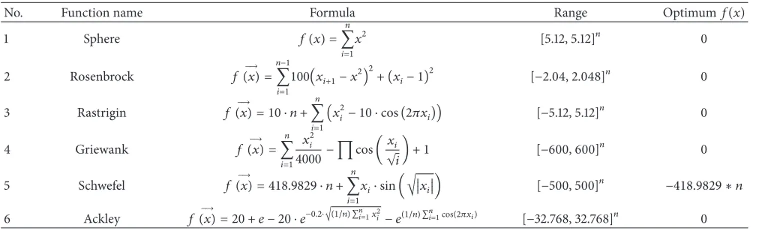
is a continuous benchmark function. However, if the bit strings are not defined and continuous, then the function is described as a discreet benchmark function [24]. Alcayde et al. [25] approach a novel extension of the well-known Pareto archived evolution strategy (PAES) which combines simu-lated annealing and tabu search. They applied this several mathematical problems show that this hybridization allows an improvement in the quality of the nondominated solutions in comparison with PAES Some of the most commonly known test functions are as follows. We have solved well-known six unconstrained single objective numeric bench-mark function. The details of the benchbench-mark functions are given inTable 1.

3. IMBO for Unconstrained Test Functions

In the original MBO mating possibility of the queen bee in the mating flight is calculated through the annealing function. In the proposed study Improved MBO (IMBO) algorithm was obtained by improving the MBO algorithm through the replacement of the annealing algorithm with the Levy flight algorithm in order to enable the queen to make a better search in the search space. Flight behaviors of many animals and insects exhibited the typical characteristics of Levy flight [26]. In addition, there are many studies to which Levy flight was successfully adapted. Pavlyukevich solved a problem of nonconvex stochastic optimization with the help of simulated annealing of Levy flights of a variable stability index [27]. In biological phenomena, Viswanathan et al. used Levy flight in the search of biologic organisms for target organisms [28]. Reynolds conducted a study by integrating Levy flight

algorithm with the honey bees’ strategies of searching food [29]. Tran et al. proposed Levy flight optimization (LFO) for global optimization problems, implemented it on the test functions, and compared the results they obtained with simulated annealing (SA) [30]. By adapting Levy flight algorithm instead of the gaussian random walk in the group search optimizer (GSO) algorithm developed for Artificial neural network (ANN), Shan applied the algorithm on a set of 5 optimization benchmark functions [31].

In general terms, Levy flight is a random walk. The steps in this random walk are obtained from Levy distribution [1]. Levy flight is implemented in 2 steps. While the first is a random selection of direction, the second is the selection of a step suitable for Levy distribution. While direction has to be selected from a homogenous distribution region, step selection is a harder process. Although there are several methods for step selection, the most effective and simplistic one is the Mantegna algorithm.

Mantegna algorithm is calculated as shown in the follow-ing equation:

𝑠 = 𝑢

|V|1/𝛽. (3)

Here, the V is obtained by taking the magnitude of the genotype as basis.

𝑢 on the other hand is calculated as shown in the following equation;

𝜎_𝑢= { Γ (1 + 𝛽) sin(𝜋𝛽/2) Γ [(1 + 𝛽) /2] 𝛽2(𝛽−1)/2}

1/𝛽

(4)

Table 1: Unconstrained test functions.

No. Function name Formula Range Optimum𝑓(𝑥)

1 Sphere 𝑓 (𝑥) = 𝑛 ∑ 𝑖=1 𝑥2 _{[5.12, 5.12]}𝑛 ₀ 2 Rosenbrock 𝑓(𝑥) =󳨀→ 𝑛−1 ∑ 𝑖=1 100(𝑥𝑖+1− 𝑥2) 2 + (𝑥𝑖− 1)2 [−2.04, 2.048]𝑛 0 3 Rastrigin 𝑓(𝑥) = 10 ⋅ 𝑛 +󳨀→ 𝑛 ∑ 𝑖=1 (𝑥2 𝑖− 10 ⋅ cos (2𝜋𝑥𝑖)) [−5.12, 5.12]𝑛 0 4 Griewank 𝑓(𝑥) =󳨀→ 𝑛 ∑ 𝑖=1 𝑥2 𝑖 4000− ∏ cos ( 𝑥𝑖 √𝑖) + 1 [−600, 600]𝑛 0 5 Schwefel 𝑓(𝑥) = 418.9829 ⋅ 𝑛 +󳨀→ 𝑛 ∑ 𝑖=1 𝑥𝑖⋅ sin (√󵄨󵄨󵄨󵄨𝑥𝑖󵄨󵄨󵄨󵄨) [−500, 500]𝑛 −418.9829 ∗ 𝑛 6 Ackley 𝑓(𝑥) = 20 + 𝑒 − 20 ⋅ 𝑒󳨀→ −0.2⋅√(1/𝑛) ∑𝑛𝑖=1𝑥𝑖2− 𝑒(1/𝑛) ∑𝑛𝑖=1cos(2𝜋𝑥𝑖) _{[−32.768, 32.768]}𝑛 ₀

While in this equation𝛽 is 0 ≤ 𝛽 ≤ 2, is the Γ is the Gamma function, and calculated as follows:

Γ (𝑧) = ∫∞

0 𝑡

𝑧−1_𝑒−𝑡_𝑑𝑡. ₍₅₎

In consequence, the direction of the next step is deter-mined with the𝑢 and V parameters, and step length is found by placing𝑢 and V into their place in the Mantegna algorithm (3). Based on𝑆, new genotype is generated as much as random genotype size, and the generated genotype is added to the previous step. Consider

𝑠 = ∝0(𝑥(𝑡)𝑗 − 𝑥(𝑡)𝑖 ) ⊕ L ́evy (𝛽) ∼ 0.01_|V|𝑢1/𝛽(𝑥(𝑡)𝑗 − 𝑥(𝑡)𝑖 ) .

(6) Creation of the new genotype of this step is completed by subjecting the new solution set obtained, that is, the genotype to the maximum and minimum controls defined for the test problem and adjusting deviations if any. Accordingly, through these implemented equations, the queen bee moves from the previous position to the next position, or towards the direction obtained from Levy distribution and by the step length obtained from Mantegna algorithm as follows:

𝐿_𝑖𝑗= 𝑥_𝑖𝑗+ 𝑠 ∗ rand (size (𝑥_𝑖𝑗)) . (7) In the crossover operator, the genotype of the queen bee and all genotypes in the current population are crossed over. Crossover was carried out by randomly calculating the number of elements subjected to crossover within Hamming distance on the genotypes to be crossed over.

In the improvement of the genotype (broods) by the worker bees single neighborhood and single inheritance from the queen was used. Consider

𝑊_𝑖𝑗= 𝑥_𝑖𝑗+ (𝑥_𝑖𝑗− 𝑥_𝑘𝑗) 0_𝑖𝑗, (8) where 0_𝑖𝑗 is a random (0, 1) value, 𝑥_𝑖 is the current brood genotype, 𝑥_𝑘 is the queen genotype, 𝑗 is a random value number of genotype. In this way, and it was observed that the developed IMBO algorithm exhibits better performance than the other metaheuristic optimization algorithms.

The MBO algorithm we modified is shown in Algorithm

2.

4. Experimental Results

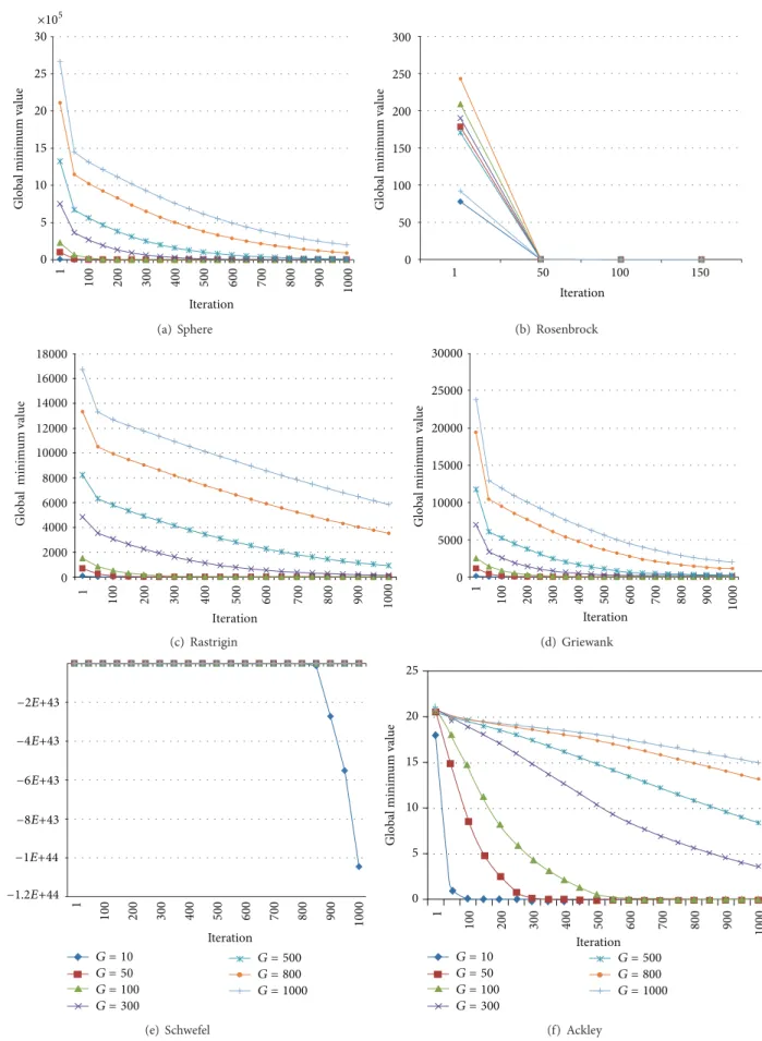
In this study, we used Sphere, Rosenbrock, Rastrigin, Griewank, Schwefel, and Ackley unconstrained test prob-lems; a program in the MatLab 2009 programming language was developed for the tests of MBO and IMBO. Genotype sizes of 10, 50, 100, 300, 500, 800, and 1000 were taken for each test. Population size (Spermatheca Size) was accepted as𝑀 = 100. At the end of each generation, mean values and standard deviations were calculated for test functions. Each genotype was developed for 10,000 generations. Each improvement was run for 30 times. Global minimum variance graphs of each test function for IMBO are presented inFigure 1.

Examining the six test functions presented in Figure 1

shows that, at first, global optimum values were far from the solution value in direct proportion to genotype size. Accordingly, for large genotypes, or in other words in cases where the number of entry parameters is high, convergence of the proposed algorithm to the optimum solution takes a longer time. The test results for MBO and IMBO are given in Tables2and3.

When Tables 2 and 3 were examined, it is seen that genotype size increases in all functions of MBO IMBO algorithms and the global minimum values get away from the optimal minimum values. InTable 2, the MBO algorithm Sphere function, 10, 50, 100 the size of genotype reached an optimum value while the other genotype sizes converge to the optimal solution. It was observed that Rosenbrock function minimum is reached optimal sizes in all genotypes. It was observed that rastrigin function 10, 50, 100, Griewank function 50, 100 genotype sizes in the optimal solution was reached. It was observed that except Schwefel function, other function and genotype sizes, the optimal solution was reached close to values.

When Table 3 was examined, it was seen that, while the size of genotype increased, IMBO algorithm Sphere, Rastrigin, Griewank, Schwefel, and Ackley function, were getting away from the optimal minimum. It was seen that Sphere function, 10, 50, 100 the size of genotype reached an optimum value while the other genotype sizes converges to the optimal solution. It was observed that, except for the size of 10 genotypes Rosenbrock function, but all other

(5)

Initialize

Randomly generate the queens Apply local search to get a good queen

Fora pre-defined maximum number of mating-flights (Maximum Iteration)

Whilespermatheca not full

Add its sperm to the queen’s spermatheca by Levy Flight (7)

End while

Generate broods by crossover and mutation

Use workers to improve the broods by single inheritance single neighborhood (8) Update workers’ fitness

Whilethe best brood is better than the worst queen Replace the least-fittest queen with the best brood Remove the best brood from the brood list

End while End for

Algorithm 2: Proposed IMBO algorithm.

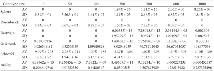
Table 2: Test results of the MBO algorithm for the genotype sizes of 10, 50, 100, 300, 500, 800, and 1000; number of runs = 30; SD: standard deviation, AV: global minimum average; generation = 10000.

Genotype size 10 50 100 300 500 800 1000 Sphere AV 0 0 0 1.97𝐸 − 26 1.21𝐸 − 13 2.06𝐸 − 06 8.26𝐸 − 04 SD 9.81𝐸 − 01 3.36𝐸 + 01 1.41𝐸 + 02 1.19𝐸 + 03 2.66𝐸 + 03 6.82𝐸 + 03 1.84𝐸 + 04 Rosenbrock AV 0 0 0 0 0 0 0 SD 4.73𝐸 − 03 8.67𝐸 − 03 8.29𝐸 − 03 1.55𝐸 − 02 7.28𝐸 − 03 8.09𝐸 − 03 0 Rastrigin AV 0 0 0 6.0633𝐸 − 13 7.88048𝐸 − 12 3.33194𝐸 − 05 0.002606 SD 0 0 0 3.95279𝐸 − 13 1.80594𝐸 − 12 3.09109𝐸 − 05 0.002843 Griewank AV 0.010377126 0 0 3.40468𝐸 − 16 7.26498𝐸 − 08 1.1388𝐸 − 06 0.000141 SD 0.026549182 0.32563139 1.09610828 8.02049039 70.78602045 36.67034057 108.177558 Schwefel AV −9.99𝐸 + 223 −2.96𝐸 + 211 −1.00𝐸 + 183 −2.37𝐸 + 306 −1.02𝐸 + 305 −1.10𝐸 + 305 −1.10𝐸 + 305 SD 3.81𝐸 + 22 1.94𝐸 + 16 5.13𝐸 + 26 4.31𝐸 + 35 7.31𝐸 + 35 3.39𝐸 + 32 7.89𝐸 + 35 Ackley AV 4.08562𝐸 − 15 8.23045𝐸 − 15 7.3922𝐸 − 09 8.49609𝐸 − 14 9.13234𝐸 − 10 0.000227233 0.000452387 SD 0.006649746 0.01783530 0.61180347 0.05005151 0.507695929 1.288113922 0.287375496

Table 3: Test results of the IMBO algorithm for the genotype sizes of 10, 50, 100, 300, 500, 800, and 1000; number of runs = 30; SD: standard deviation, AV: global minimum average; generation = 10000.

Genotype size 10 50 100 300 500 800 1000 Sphere AV 0 0 0 1.38𝐸 − 28 1.47𝐸 − 13 2.78𝐸 − 07 0.0001224 SD 0 0 0 8.97𝐸 − 29 1.90𝐸 − 15 8.50𝐸 − 08 3.09𝐸 − 05 Rosenbrock AV 2.25𝐸 − 07 0 0 0 0 0 0 SD 2.24𝐸 − 06 0 0.1425029 0 0 0.2440021 0 Rastrigin AV 0 0 4.54𝐸 − 15 5.68𝐸 − 13 3.60𝐸 − 12 6.13𝐸 − 07 0.0002386 SD 0 0 3.18𝐸 − 14 4.78𝐸 − 13 1.25𝐸 − 12 3.14𝐸 − 07 9.13𝐸 − 05 Griewank AV 0.0002219 0 0 3.48𝐸 − 16 9.15𝐸 − 13 1.78𝐸 − 07 3.26𝐸 − 05 SD 0.0012617 0 0 3.85𝐸 − 17 1.88𝐸 − 14 5.43𝐸 − 08 6.73𝐸 − 06 Schwefel AV −1.21𝐸 + 23 −1.08𝐸 + 25 −6.17𝐸 + 29 −1.21𝐸 + 40 −1.76𝐸 + 36 −2.96𝐸 + 39 −1.64𝐸 + 39 SD 7.28𝐸 + 44 1.06𝐸 + 26 3.52𝐸 + 30 6.52𝐸 + 40 5.78𝐸 + 36 2.14𝐸 + 40 1.49𝐸 + 40 Ackley AV 3.73𝐸 − 15 8.13𝐸 − 15 1.57𝐸 − 14 7.49𝐸 − 14 1.76𝐸 − 05 3.30𝐸 − 05 0.0006221 SD 1.42𝐸 − 15 9.94𝐸 − 16 2.30𝐸 − 15 5.11𝐸 − 15 3.09𝐸 − 05 9.57𝐸 − 06 0.0001513

(6)

0 5 10 15 20 25 30 1 100 200 300 400 500 600 700 800 900 ₁₀₀₀ Iteration Global minim um val ue ×105 (a) Sphere 0 50 100 150 200 250 300 1 50 100 150 Iteration Global minim um val ue (b) Rosenbrock 0 2000 4000 6000 8000 10000 12000 14000 16000 18000 1 100 200 300 400 500 600 700 800 900 ₁₀₀₀ Iteration Global minim um value (c) Rastrigin 1 100 200 300 400 500 600 700 800 900 ₁₀₀₀ Iteration 0 5000 10000 15000 20000 25000 30000 Global minim um val ue (d) Griewank −8E+43 −6E+43 −4E+43 −2E+43 1 100 200 300 400 500 600 700 800 900 ₁₀₀₀ Iteration Global minim um val ue G = 10 G = 50 G = 100 G = 300 G = 500 G = 800 G = 1000 −1.2E+44 −1E+44 (e) Schwefel 25 20 15 10 5 0 G = 10 G = 50 G = 100 G = 300 G = 500 G = 800 G = 1000 Global minim um val ue 1 100 200 300 400 500 600 700 800 900 ₁₀₀₀ Iteration (f) Ackley

Figure 1: Mean global minimum convergence graphs of benchmark functions in 1000 generations for genotype sizes(𝐺) of 10, 50, 100, 300, 500, 800 and 1000.

(7)

Table 4: Success rates of MBO when compared with those of the IMBO algorithm. + indicates that the algorithm is better while− indicates that it is worse than the other. If both algorithms show similar performance, they are both +.

Genotype size 10 50 100 300 500 800 1000

Function MBO IMBO MBO IMBO MBO IMBO MBO IMBO MBO IMBO MBO IMBO MBO IMBO

Sphere + + + + + + − + + − − + − + Rosenbrock + − + + + + + + + + + + + + Rastrigin + + + + + − − + − + − + − + Griewank − + + + + + + − − + − + − + Schwefel − + − + − + − + − + − + − + Ackley − + − + − + − + + − − + + − Total 3 5 4 6 4 5 2 5 3 4 1 6 2 5

Table 5: CPU time results of the MBO algorithm for the genotype sizes of 10, 50, 100, 300, 500, 800, and 1000; number of runs = 1; iteration = 10000.

Genotype size Sphere Rosenbrock Rastrigin Griewank Schwefel Ackley

10 02:45:095 02:36:827 03:12.552 05:00.894 03:25.141 03:20.882 50 05:39:832 05:35.729 06:15.572 08:22.590 07:30.842 06:20.845 100 15:47:269 17:13.912 17:36.329 18:34.517 17:29.746 15:55:318 300 1:09:07:083 1:07:07.602 1:12:21.617 1:16:02.748 1:17:11.700 1:16:04.994 500 2:03:31:669 2:03:54.118 2:08:22.112 2:03:11.670 2:06:25.689 2:09:27.164 800 3:23:52:834 2:51:14.834 2:53:25.547 3:00:11.898 3:06:41.792 2:52:34.737 1000 4:31:56.752 3:35:18.224 3:40:03.753 3:45:45.894 3:54:20.884 3:38:12.446

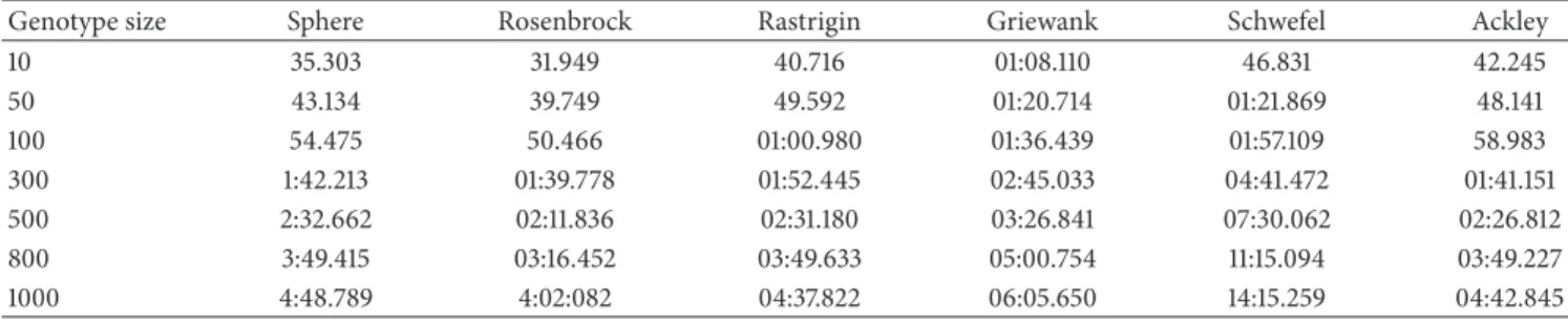
Table 6: CPU time results of the IMBO algorithm for the genotype sizes of 10, 50, 100, 300, 500, 800, and 1000; number of runs = 1; iteration = 10000.

Genotype size Sphere Rosenbrock Rastrigin Griewank Schwefel Ackley

10 35.303 31.949 40.716 01:08.110 46.831 42.245 50 43.134 39.749 49.592 01:20.714 01:21.869 48.141 100 54.475 50.466 01:00.980 01:36.439 01:57.109 58.983 300 1:42.213 01:39.778 01:52.445 02:45.033 04:41.472 01:41.151 500 2:32.662 02:11.836 02:31.180 03:26.841 07:30.062 02:26.812 800 3:49.415 03:16.452 03:49.633 05:00.754 11:15.094 03:49.227 1000 4:48.789 4:02:082 04:37.822 06:05.650 14:15.259 04:42.845

genotypes sizes optimal minimum was reached. Rastrigin function 10, 50, Griewank function 50, 100 to the optimal solution was observed to have reached the optimal solution. The other functions and sizes of genotype were observed to have reached the values close to the optimal solution.

Comparative results of the best and mean solutions of the MBO and IMBO algorithms are presented inTable 4.

According to Table 4, it is seen that, when compared with the MBO algorithm and IMBO algorithm according to genotype, IMBO exhibited better performance than MBO in all genotypes sizes. When it was thought that total better or equal cases were represented with “+” mark, MBO algorithm, a total of 19 “+” available, and IMBO algorithm, a total of 36 pieces of the “+” were available. Accordingly, IMBO’s MBO algorithm demonstrates a better performance.

CPU time results of the all genotype sizes for MBO are given inTable 5and for IMBO are given inTable 6.

In Tables 5 and 6, it was seen that, when CPU time values were analyzed, depending upon the size in the same

proportion as genotype problem, solving time took a long time. Again in these tables, when solution CPU time of MBO and IMBO algorithm was analyzed, IMBO algorithm solves problems with less CPU time than MBO algorithm.

For 10, 50, 100, and 1000 problem sizes of unconstrained numeric six benchmark functions, comparisons were made between test results of IMBO algorithm and the algorithms in literature, including DE, PSO, ABC [32], bee swarm optimization, (BSO) [33], bee and foraging algorithm (BFA) [34], teaching-learning-based optimization (TLBO) [35], bumble bees mating optimization (BBMO) [36] and honey bees mating optimization algorithm (HBMO) [36].Table 7

presents the comparison between experimental test results obtained for 10-sized genotype (problem) on unconstrained test functions of IMBO algorithm and the results for the same problem size in literature including PSO, DE, ABC, BFA and BSO optimization algorithms; while the comparison of success of each algorithm and IMBO algorithm is given in

(8)

Table 7: The mean solutions obtained by the PSO, DE, ABC, BFA, BSO, and IMBO algorithms for 6 test functions over 30 independent runs and total success numbers of algorithms. Genotype size: 10; (—): not available value, SD: standard deviation, AV: global minimum average.

Problem PSO DE ABC IMBO BFA BSO

Sphere ORT 4.13𝐸 − 17 4.41𝐸 − 17 4.88𝐸 − 17 0 0.000031 8.475𝐸 − 123 SD 7.71𝐸 − 18 8.09𝐸 − 18 5.21𝐸 − 18 0 0.00024 3.953𝐸 − 122 Rosenbrock ORT 0.425645397 4.22𝐸 − 17 0.013107593 2.25𝐸 − 07 7.2084513 3.617𝐸 − 7 SD 1.187984439 1.09𝐸 − 17 0.008658828 2.24𝐸 − 06 9.436551 5.081𝐸 − 5 Rastrigin ORT 7.362692992 0.099495906 4.76𝐸 − 17 0 0.003821 4.171𝐸 − 64 SD 2.485404145 0.298487717 4.40𝐸 − 18 0 0.006513 7.834𝐸 − 64 Griewank ORT 0.059270504 0.008127282 5.10𝐸 − 19 0.000221881 3.209850 3.823𝐸 − 46 SD 0.03371245 0.009476456 1.93𝐸 − 19 0.00126167 4.298031 6.679𝐸 − 46 Schwefel ORT −2654.033431 −4166.141206 −4189.828873 −1.21𝐸 + 23 — — SD 246.5263242 47.37533385 9.09𝐸 − 13 7.289𝐸 + 44 — — Ackley ORT 4.67𝐸 − 17 4.86𝐸 − 17 1.71𝐸 − 16 3.73𝐸 − 15 0.000085 7.105𝐸 − 19 SD 8.06𝐸 − 18 6.55𝐸 − 18 3.57𝐸 − 17 1.42𝐸 − 15 0.000237 5.482𝐸 − 18

Table 8: Comparative results of IMBO with PSO, DE, ABC, BFA, and BSO algorithms over 30 independent runs for genotype size 50. + indicates that the algorithm is better while− indicates that it is worse than the other, (—): not available value. If both algorithms show similar performance, they are both +.

Problem IMBO-PSO IMBO-DE IMBO-ABC IMBO-BFA IMBO-BSO

IMBO PSO IMBO DE IMBO ABC IMBO BFA IMBO BSO

Sphere + − + − + − + − + − Rosenbrock + − − + + − + − + − Rastrigin + − + − + − + − + − Griewank + − + − − + + − − + Schwefel − + − + − + — — — — Ackley − + − + − + + − − + Total 4 2 3 3 3 3 5 0 3 2

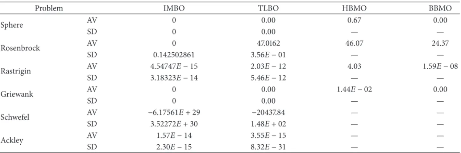
Table 9: The mean solutions obtained by the TLBO, HBMO, BBMO, and IMBO algorithms for 6 test functions over 30 independent runs and total success numbers of algorithms. Genotype size: 50; (—): not available value, SD: standard deviation, AV: global minimum average.

Problem IMBO TLBO HBMO BBMO

Sphere AV 0 0.00 0.67 0.00 SD 0 0.00 — — Rosenbrock AV 0 47.0162 46.07 24.37 SD 0.142502861 3.56𝐸 − 01 — — Rastrigin AV 4.54747𝐸 − 15 2.03𝐸 − 12 4.03 1.59𝐸 − 08 SD 3.18323𝐸 − 14 5.46𝐸 − 12 — — Griewank AV 0 0.00 1.44𝐸 − 02 0.00 SD 0 0.00 — — Schwefel AV −6.17561𝐸 + 29 −20437.84 — — SD 3.52272𝐸 + 30 1.48𝐸 + 02 — — Ackley AV 1.57𝐸 − 14 3.55𝐸 − 15 — — SD 2.30𝐸 − 15 8.32𝐸 − 31 — —

test results obtained for 50-sized genotype (problem) on unconstrained test functions of IMBO algorithm and the results for the same problem size in literature including TLBO, HBMO and BBMO optimization algorithms, while the comparison of success of each algorithm and IMBO algorithm is given inTable 10.Table 11shows the comparison between experimental test results for 100-sized genotype

(problem) on unconstrained test functions of IMBO algo-rithm and the results for the same problem size in literature including PSO, DE, and ABC optimization algorithms, while the comparison of success of each algorithm and IMBO algorithm is given in Table 12. Table 13shows the compar-ison between experimental test results obtained for 1000-sized genotype (problem) on unconstrained test functions of

(9)

Table 10: Comparative results of IMBO with TLBO, HBMO, and BBMO algorithms over 30 independent runs for genotype size 50. + indicates that the algorithm is better while− indicates that it is worse than the other, (—): not available value. If both algorithms show similar performance, they are both +.

Problem IMBO-TLBO IMBO-HBMO IMBO-BBMO

IMBO TLBO IMBO HBMO IMBO BBMO

Sphere + − + − + + Rosenbrock + − + − + − Rastrigin + − + − + − Griewank + + + − + + Schwefel − + — — — — Ackley − + — — — — Total 4 3 4 0 4 2

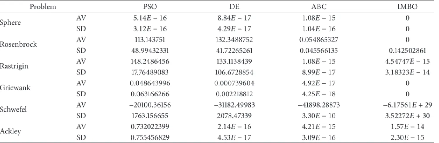
Table 11: The mean solutions obtained by the DE, PSO, ABC, and IMBO algorithms for 6 test functions over 30 independent runs and total success numbers of algorithms. Genotype size: 100; (—): not available value, SD: standard deviation, AV: global minimum average.

Problem PSO DE ABC IMBO

Sphere AV 5.14𝐸 − 16 8.84𝐸 − 17 1.08𝐸 − 15 0 SD 3.12𝐸 − 16 4.29𝐸 − 17 1.04𝐸 − 16 0 Rosenbrock AV 113.143751 132.3488752 0.054865327 0 SD 48.99432331 41.72265261 0.045566135 0.142502861 Rastrigin AV 148.2486456 133.1138439 1.08𝐸 − 15 4.54747𝐸 − 15 SD 17.76489083 106.6728854 8.99𝐸 − 17 3.18323𝐸 − 14 Griewank AV 0.048643996 0.000739604 4.92𝐸 − 17 0 SD 0.063166266 0.002218812 4.25𝐸 − 18 0 Schwefel AV −20100.36156 −31182.49983 −41898.28873 −6.17561𝐸 + 29 SD 1763.156655 2078.47339 3.30𝐸 − 10 3.52272𝐸 + 30 Ackley AV 0.732022399 2.14𝐸 − 16 4.21𝐸 − 15 1.57𝐸 − 14 SD 0.755456829 4.53𝐸 − 17 3.09𝐸 − 16 2.30𝐸 − 15

Table 12: Comparative results of IMBO with DE, PSO, and ABC algorithms over 30 independent runs for genotype size 100. + indicates that the algorithm is better while− indicates that it is worse than the other. If both algorithms show similar performance, they are both +.

Problem IMBO-PSO IMBO-DE IMBO-ABC

IMBO PSO IMBO DE IMBO ABC

Sphere + − + − + Rosenbrock + − + − + Rastrigin + − + − − + Griewank + − + − + − Schwefel − + − + − + Ackley + − + − − + Total 5 1 5 1 3 3

IMBO algorithm and the results for the same problem size in the literature including PSO, DE, and ABC optimization algo-rithms, while the comparison of success of each algorithm and IMBO algorithm is given inTable 14.

Tables7,11, and13demonstrate that, as the problem size increases in ABC, DE, and PSO, the solution becomes more distant and difficult to reach. However, the results obtained with IMBO showed that, despite the increasing problem size, optimum value could be obtained or converged very closely. There are big differences among the results obtained for 10, 100, and 1000 genotype sizes in DE and PSO; however, this

difference is smaller in IMBO algorithm, which indicates that IMBO performs better even in large problem sizes. In Tables

7and 8, it is seen that IMBO performs equally to DE and ABC and better than PSO, BFA and BSO. In Tables9 and

10showing the comparison of IMBO with LBO, HBMO, and BBMO for genotype (problem) size 50, it is seen that IMBO performs better than all the other algorithms. In Tables11and

12showing the comparison of IMBO with DE, PSO and ABC algorithms on problem size 100, it is seen that IMBO performs equally to ABC and better than DE and PSE. In Tables13and

(10)

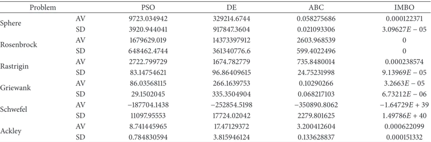
Table 13: The mean solutions obtained by the DE, PSO, ABC, and IMBO algorithms for 6 test functions over 30 independent runs and total success numbers of algorithms. Genotype size: 1000; (—): not available value, SD: standard deviation, AV: global minimum average.

Problem PSO DE ABC IMBO

Sphere AV 9723.034942 329214.6744 0.058275686 0.000122371 SD 3920.944041 917847.3604 0.021093306 3.09627𝐸 − 05 Rosenbrock AV 1679629.019 14373397912 2603.968539 0 SD 648462.4744 361340776.6 599.4022496 0 Rastrigin AV 2722.799729 1674.782779 735.8480014 0.000238574 SD 83.14754621 96.86409615 24.75231998 9.13969𝐸 − 05 Griewank AV 86.03568115 266.1639753 0.10290266 3.2663𝐸 − 05 SD 29.1502045 335.3504904 0.068217103 6.73212𝐸 − 06 Schwefel AV −187704.1438 −252854.5198 −350890.8062 −1.64729𝐸 + 39 SD 11097.95553 17724.02042 2279.801625 1.49786𝐸 + 40 Ackley AV 8.741445965 17.47129372 3.200412604 0.000622099 SD 0.784830594 3.815946124 0.133628837 0.000151332

Table 14: Comparative results of IMBO with DE, PSO, and ABC algorithms over 30 independent runs for genotype size 1000. + indicates that the algorithm is better while− indicates that it is worse than the other. If both algorithms show similar performance, they are both +.

Problem IMBO-PSO IMBO-DE IMBO-ABC

IMBO PSO IMBO DE IMBO ABC

Sphere + − + − + − Rosenbrock + − + − + − Rastrigin + − + − + − Griewank + − + − + − Schwefel − + − + − + Ackley + − + − + − Total 5 1 5 1 5 1

on problem size 1000, IMBO is seen to perform better than all the other algorithms.

5. Conclusion

In the proposed study, we developed a new IMBO by replacing annealing algorithm in the queen bee’s mating flight with the Levy flight algorithm and using single inheritance and single neighborhood in the genotype improvement stage. We tested the MBO algorithm we improved on the most commonly known six unconstrained numeric benchmark functions. We compared the results obtained with the results of other metaheuristic optimization algorithms in the litera-ture for the same test functions.

In order to observe the improvement of IMBO, the experimental test results of MBO and IMBO were compared for 10, 50, 100, 300, 500, 800, and 1000 problem sizes. Consequently, IMBO algorithm was concluded to perform better than MBO algorithm. Furthermore, according to CPU time of problem solving process, IMBO algorithm works in shorter CPU times. The test results obtained with IMBO were compared with the results of DE, ABC, PSO, BSO, BFA; TLBO, BBMO and HBMO in the literature.

Accordingly, IMBO is observed to perform equally to or a little better than other algorithms in comparison with small genotype size, while IMBO performs much better than other

algorithms with large genotype size. A total of 14 comparisons were made between experimental results of IMBO and other optimization algorithms in literature, and it showed better performances in 11 comparisons, and equal performances in 3 comparisons.

In future studies, different improvements can be made on the MBO algorithm and tests can be made on different test functions. Also, comparisons can be made with other meta-heuristic optimization algorithms not used in the present study.

References

[1] X.-S. Yang, “Levy flight,” in Nature-Inspired Metaheuristic Algo-rithms, pp. 14–17, Luniver Press, 2nd edition, 2010.

[2] D. Bunnag and M. Sun, “Genetic algorithm for constrained global optimization in continuous variables,” Applied Mathe-matics and Computation, vol. 171, no. 1, pp. 604–636, 2005. [3] H. E. Romeijn and R. L. Smith, “Simulated annealing for

con-strained global optimization,” Journal of Global Optimization, vol. 5, no. 2, pp. 101–126, 1994.

[4] J. Kennedy and R. Eberhart, “Particle swarm optimization,” in Proceedings of the IEEE International Conference on Neural Networks, pp. 1942–1948, December 1995.

[5] J. Holland, Adaptation in Natural and Artificial Systems, Univer-sity of Michigan Press, 1975.

(11)

[6] R. Storn and K. Price, “Differential evolution—a simple and efficient heuristic for global optimization over continuous spaces,” Journal of Global Optimization, vol. 11, no. 4, pp. 341– 359, 1997.

[7] O. B. Haddad, A. Afshar, and M. A. Mari˜no, “Honey-bees mating optimization (HBMO) algorithm: a new heuristic approach for water resources optimization,” Water Resources Management, vol. 20, no. 5, pp. 661–680, 2006.

[8] H. A. Abbass, “MBO: Marriage in honey bees optimization a haplometrosis polygynous swarming approach,” in Proceedings of the Congress on Evolutionary Computation (CEC ’01), pp. 207– 214, May 2001.

[9] T. Thomas, Evolutionary Algorithms in Theory and Practice: Evolution Strategies, Evolutionary Programming, Genetic Algo-rithms, Oxford University Press, New York, NY, USA, 1996. [10] C. Coello Coello and G. B. Lamont, Evolutionary Algorithms for

Solving Multi-Objective Problems, Genetic Algorithms and Evo-lutionary Computation, Kluwer Academic Publishers, Boston, Mass, USA, 2nd edition, 2007.

[11] D. Karaboga and B. Basturk, “On the performance of artificial bee colony (ABC) algorithm,” Applied Soft Computing Journal, vol. 8, no. 1, pp. 687–697, 2008.

[12] J. G. Digalakis and K. G. Margaritis, “On benchmarking func-tions for genetic algorithms,” International Journal of Computer Mathematics, vol. 77, no. 4, pp. 481–506, 2001.

[13] M. M. Hassan, F. Karray, M. S. Kamel, and A. Ahmadi, “An inte-gral approach for Geno-Simulated Annealing,” in Proceedings of the 10th International Conference on Hybrid Intelligent Systems (HIS ’10), pp. 165–170, August 2010.

[14] A. Chatterjee and P. Siarry, “Nonlinear inertia weight variation for dynamic adaptation in particle swarm optimization,” Com-puters and Operations Research, vol. 33, no. 3, pp. 859–871, 2006. [15] R. S. Rahnamayan, H. R. Tizhoosh, and M. M. A. Salama, “Opposition-based differential evolution,” IEEE Transactions on Evolutionary Computation, vol. 12, no. 1, pp. 64–79, 2008. [16] H. A. Abbass and J. Teo, “A true annealing approach to the

marriage in honey-bees optimization algorithm,” International Journal of Computational Intelligence and Aplications, vol. 3, pp. 199–208, 2003.

[17] H. S. Chang, “Converging marriage in honey-bees optimization and application to stochastic dynamic programming,” Journal of Global Optimization, vol. 35, no. 3, pp. 423–441, 2006. [18] A. Afshar, O. Bozorg Haddad, M. A. Mari˜no, and B. J. Adams,

“Honey-bee mating optimization (HBMO) algorithm for opti-mal reservoir operation,” Journal of the Franklin Institute, vol. 344, no. 5, pp. 452–462, 2007.

[19] Y. Marinakis, M. Marinaki, and G. Dounias, “Honey bees mating optimization algorithm for the Euclidean traveling salesman problem,” Information Sciences, vol. 181, no. 20, pp. 4684–4698, 2011.

[20] C.-Y. Chiu and T. Kuo, “Applying honey-bee mating optimiza-tion and particle swarm optimizaoptimiza-tion for clustering problems,” Journal of the Chinese Institute of Industrial Engineers, vol. 26, no. 5, pp. 426–431, 2009.

[21] D. Karaboga and B. Basturk, “A powerful and efficient algo-rithm for numerical function optimization: artificial bee colony (ABC) algorithm,” Journal of Global Optimization, vol. 39, no. 3, pp. 459–471, 2007.

[22] R. F. A. Moritzl and C. Brandesl, “Behavior genetics of hon-eybees (Apis mellifera L.),” in Neurobiology and Behavior of Honeybees, pp. 21–35, Springer, Berlin, Germany, 1987.

[23] R. F. A. Moritz and E. E. Southwick, Bees as Super-Organisms, Springer, Berlin, Germany, 1992.

[24] B. Bilgin, E. ¨Ozcan, and E. E. Korkmaz, “An experimental study on hyper-heuristics and exam scheduling,” in Practice and Theory of Automated Timetabling VI, vol. 3867 of Lecture Notes in Computer Science, pp. 394–412, Springer, 2007.

[25] A. Alcayde, R. Ba˜nos, C. Gil, F. G. Montoya, J. Moreno-Garcia, and J. G´omez, “Annealing-tabu PAES: a multi-objective hybrid meta-heuristic,” Optimization, vol. 60, no. 12, pp. 1473–1491, 2011.

[26] X.-S. Yang and S. Deb, “Multiobjective cuckoo search for design optimization,” Computers and Operations Research, vol. 40, no. 6, pp. 1616–1624, 2013.

[27] I. Pavlyukevich, “L´evy flights, non-local search and simulated annealing,” Journal of Computational Physics, vol. 226, no. 2, pp. 1830–1844, 2007.

[28] G. M. Viswanathan, F. Bartumeus, and S. V. Buldyrev, “Levy Flight random searches in biological phenomena,” Physica A, vol. 314, pp. 208–213, 2002.

[29] A. M. Reynolds, “Cooperative random L´evy flight searches and the flight patterns of honeybees,” Physics Letters A, vol. 354, no. 5-6, pp. 384–388, 2006.

[30] T. T. Tran, T. T. Nguyen, and H. L. Nguyen, “Global optimization using levy flight,” in Proceedings of the 3rd National Symposium on Research, Development and Application of Information and Communication Technology (ICT.rda ’06), Hanoi, Vietnam, September 2004.

[31] S. He, “Training artificial neural networks using l´evy group search optimizer,” Journal of Multiple-Valued Logic and Soft Computing, vol. 16, no. 6, pp. 527–545, 2010.

[32] B. Akay, Nimerik Optimizasyon Problemlerinde Yapay Arı Kolonisi (Artifical Bee Colony, ABC) Algoritmasının Performans Analizi, Kayseri ¨Universitesi, Fen Bilimleri Enstit¨us¨u, Kayseri, Turkey, 2009.

[33] R. Akbari, A. Mohammadi, and K. Ziarati, “A novel bee swarm optimization algorithm for numerical function optimization,” Communications in Nonlinear Science and Numerical Simula-tion, vol. 15, no. 10, pp. 3142–3155, 2010.

[34] K. Sundareswaran and V. T. Sreedevi, “Development of novel optimization procedure based on honey bee foraging behavior,” in Proceedings of the IEEE International Conference on Systems, Man and Cybernetics (SMC ’08), pp. 1220–1225, October 2008. [35] R. Venkata Rao and V. Patel, “An improved

teaching-learning-based optimization algorithm for solving unconstrained opti-mization problems,” Scientia Iranica. In press.

[36] Y. Marinakis, M. Marinaki, and N. Matsatsinis, “A bumble bees mating optimization algorithm for global unconstrained optimization problems,” Studies in Computational Intelligence, vol. 284, pp. 305–318, 2010.

(12)

Submit your manuscripts at

http://www.hindawi.com

Computer Games Technology

International Journal of

Hindawi Publishing Corporation

http://www.hindawi.com Volume 2014

http://www.hindawi.com Volume 2014 Distributed Sensor Networks International Journal of Advances in

Fuzzy

Systems

International Journal of Reconfigurable Computing

Applied

Computational

Intelligence and Soft

Computing

Advances in

Artificial

Intelligence

Hindawi Publishing Corporation http://www.hindawi.com Volume 2014 Advances in Software Engineering

http://www.hindawi.com Volume 2014 Electrical and Computer Engineering

Journal of

Computer Networks and Communications

Hindawi Publishing Corporation

http://www.hindawi.com Volume 2014

Multimedia

International Journal of

Biomedical Imaging

Artificial

Neural Systems

Advances in

Robotics

Journal of

http://www.hindawi.com Volume 2014 Hindawi Publishing Corporationhttp://www.hindawi.com Volume 2014 Computational Intelligence and Neuroscience

Modelling & Simulation in Engineering

The Scientific

World Journal

Human-Computer Interaction

Advances in

Computer EngineeringAdvances in