c
⃝ T¨UB˙ITAK doi:10.3906/fiz-1211-3 h t t p : / / j o u r n a l s . t u b i t a k . g o v . t r / p h y s i c s /
Research Article
Theoretical modeling and numerical solutions of some standard
thermoluminescence detector crystals
Erdem UZUN∗
Department of Physics, Karamano˘glu Mehmetbey University, Karaman, Turkey
Received: 06.11.2012 • Accepted: 14.03.2013 • Published Online: 13.09.2013 • Printed: 07.10.2013
Abstract: MCP-100, MYS-N, MTS-7, MTS-100, and MCP-N standard thermoluminescence detector materials are
annealed and irradiated. Glow curves and all trap parameters are determined. For these materials new theoretical energy band models are suggested and differential equations governing the charge carrier traffics are derived. The equations are solved by using computer-based numerical methods. During the simulations, experimental data measured in the previous step are given to computer code as the initial conditions. Experimental and numerical results show that the electron-band structures of standard thermoluminescence crystals are represented fairly well by the suggested models.
Key words: Thermoluminescence, trap parameters, numeric solutions
1. Introduction
Thermoluminescence (TL) is an established method for radiation dosimetry and in spite of its great success different difficulties are associated with its application [1–3]. The main problem is the calculation of the fundamental trap parameters [4]. To overcome this problem, TL models and their exact or the nearest solutions must be present. For this purpose, lots of numerical solutions are reported by researchers in the literature. Firstly, a graphical method was given by Cowell and Woods [5] for evaluating the activation energy. In essence, the method of determining the trapping parameters utilizes some equations derived by the researchers. They reported that an excellent fit between the theoretical and experimental curves was obtained by using the proposed method. They also illustrated its application to some experimental results obtained from CdS crystals, but the method is very long and complex. A numerical method has been also given by Mohan and Chen [6,7]. Their procedure for this was as follows. Once the glow curve is measured, an estimate for E is obtained by using one of the known methods and a theoretical curve is plotted. Then maximum intensity is adjusted so that the experimental and theoretical curves coincide. The fitting of the rest of the curve is then checked. A value of E is chosen and the procedure is repeated until the desired fit is obtained. Their method was checked both for numerically generated peaks and experimental TL curves of NaCl and ZnS:Er3+ samples. They reported
that results are in good agreement with the given values of activation energies in the former case and values calculated. Moscovitcht et al. [8] described a computerized first-order kinetics glow peak analysis technique that involves electronic transfer of the glow curve data to a microprocessor followed by first-order kinetic analysis of peaks. However, this technique is suggested only for LiF TL crystals. Bull [9] suggested and solved numerically the system of rate equations that describes the localized transition model. By using this model 2 extreme cases
were studied. Firstly transitions to and from the conduction band were neglected and only localized transitions allowed. Secondly this restriction was lifted and the competition between TL transitions from the conduction band and the excited state was examined. The equations were solved by using a special computer code and thus first-order glow curves were obtained for the entire trap parameters. Sunta et al. [10] calculated numerically TL glow peaks for a one-trap-one-recombination-center model using a generalized approach. It this method, glow peaks are fitted to the general-order kinetics model and the values of the kinetic parameters are determined by finding the best fit. Singh et al. [11] have proposed a modification of the existing equation of mixed-order kinetics. In their study, a new set of expressions was presented for the evaluation of the activation energy. Vejnovic et al. [12] introduced a new approach in which the equation that describes general-order kinetics is an interpolating function between analogous equations for first- and second-order kinetics. They also proposed a new theoretical method for calculation of parameters and the method is based on the determination of the glow curve maximum, and the effective values of half-width and part of the half-width on the higher temperature side. Similar studies have been conducted by many others [13–34]. It is clear from the above literature that there are some general constraints used in all these studies. In addition, these methods are rather long and troublesome and therefore it is not possible to obtain accurate results. For these purposes, in this work, computer-based new numerical solutions are performed but no simplifications are used.
2. Thermoluminescence models
Randall and Wilkins [35,36], Garlick and Gibson [37], May and Partigle [38], and many others [39,40] gave analytical descriptions of glow peaks. According to these models, the shape, position, and intensity of glow peaks are related to various trapping parameters. These parameters include the order of kinetics (b), the activation energy E (eV), the frequency factor S (s−1) , and the heating rates β (K s−1) [1,2,6]. Detailed information about the models can be found in the literature [1,2,35–40].
2.1. The method
Numerical solutions of the differential equations by using computer code are an objective and accurate method for evaluating trap parameters. In addition, using the numerical solutions of the differential equations not only for first-order kinetics but also the method is extended to the case of second- or mixed-order kinetics.
In this paper, differential equations governing the charge carrier traffic for all the TL models mentioned above are solved numerically by using special code running on the Mathematica 8.0 computer program. Sim-ulations are done in 3 stages. The first stage is the filling of traps; in this stage the filling of traps under a given intensity of an ionizing radiation is discussed. At the end of this stage, free charge carriers generated by irradiation in the conduction and valence bands are presented. The second stage is relaxation; during this stage the differential equations present the relationships between the number (per unit volume) of electrons in the conduction band nc(T, t) and traps n (T,t), holes in the valence band nv(T, t) and recombination centers r(T, t) , all as functions of time and temperature. At the end of this stage there are no electrons in the conduc-tion band and all electrons are trapped by electron trap levels or recombinaconduc-tion centers. The third stage is the heating stage; in this stage the excitation of the sample is carried out when the temperature of the specimen is high enough so that trapped electrons are raised thermally to the conduction band.
2.2. Theoretical modeling and experimental comparisons
In this section, firstly experimental glow curves of some standard TL detector crystals were performed, the numbers of trap energy levels were determined, and experimental trap parameters were calculated. For these
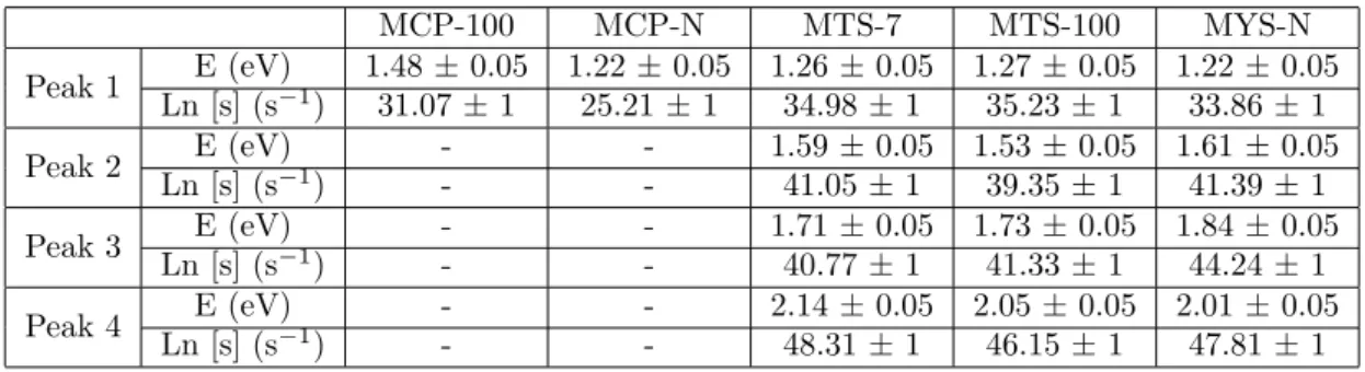
purposes, MCP-100 (LiF: Mg, Cu, P), MYS-N (LiF-N: Mg, Ti), MTS-7 (LiF: Mg, Ti, 7Li-enriched), MTS-100 (LiF: Mg, Ti), and MCP-N (LiF: Mg, Cu, P, natural abundance) (http://www.tld.com.pl/tld/products.html) standard TL detector crystals were annealed at 400 ◦C for 5 min and thus the effect of residual radiation was eliminated. Then the crystals were cooled to room temperature and were irradiated by Sr-90 beta source. Full glow curves of the irradiated crystals were obtained by using a semiautomatic TLD reader model RE-2000-s system in Karamano˘glu Mehmetbey University Department of Physics TL laboratory. All glow curves were analyzed by computerized glow curve deconvolution [41–43] and all trap parameters were determined. Experimental trap parameters are summarized in the Table.
Table. Experimental trap parameters of the standard dosimeter crystals.
MCP-100 MCP-N MTS-7 MTS-100 MYS-N Peak 1 E (eV) 1.48± 0.05 1.22 ± 0.05 1.26 ± 0.05 1.27 ± 0.05 1.22 ± 0.05 Ln [s] (s−1) 31.07± 1 25.21± 1 34.98± 1 35.23± 1 33.86± 1 Peak 2 E (eV) - - 1.59± 0.05 1.53 ± 0.05 1.61 ± 0.05 Ln [s] (s−1) - - 41.05± 1 39.35± 1 41.39± 1 Peak 3 E (eV) - - 1.71± 0.05 1.73 ± 0.05 1.84 ± 0.05 Ln [s] (s−1) - - 40.77± 1 41.33± 1 44.24± 1 Peak 4 E (eV) - - 2.14± 0.05 2.05 ± 0.05 2.01 ± 0.05 Ln [s] (s−1) - - 48.31± 1 46.15± 1 47.81± 1
Then, in the light of the experimental results, new theoretical energy-band models were suggested for each standard crystal. Model 1 was suggested for MCP-100 and MCP-N; it has only 1 electron trap center. Model 2 was suggested for MTS-7, MTS-100, and MYS-N; it has 4 electron trap centers. The models are shown in Figure 1, where Ei is the trap depth of the ith trap, si is the frequency to escape, and Ani is the probability of transitions. E1,S1,N1 E2,S2,N2 E3,S3,N3 E4,S4,N4 An1 An2 An3 An4 Ah Ar Eh,Sh,Nh
C. B.
V. B.
E1,S1,N An1 Ah Ar Eh,Sh,NhC. B.
V. B.
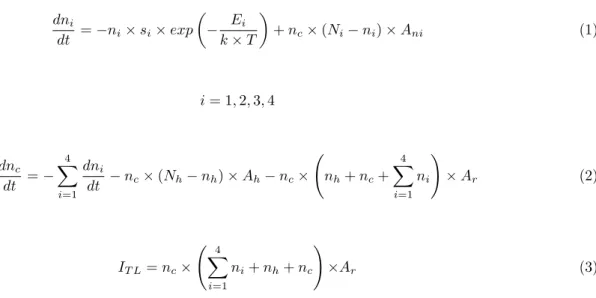
E r E r Model 1 Model 2 Nr , ,NrIn addition, differential equations governing the charge carrier traffics were derived for each model. The equations are generalized and presented in Eqs. (1)–(3).
dni dt =−ni× si× exp ( − Ei k× T ) + nc× (Ni− ni)× Ani (1) i = 1, 2, 3, 4 dnc dt =− 4 ∑ i=1 dni dt − nc× (Nh− nh)× Ah− nc× ( nh+ nc+ 4 ∑ i=1 ni ) × Ar (2) IT L= nc× ( 4 ∑ i=1 ni+ nh+ nc ) ×Ar (3)
Then numerical solutions of these equations were performed via a special code running on the Mathematica 8.0 computer program with the initial conditions given in the Table for each crystal. Experimental and numerical glow curves are presented in Figure 2.
100 200 300 400 0 1×10⁷ 2×10⁷ 3×10⁷ 4×10⁷ ITL Experiment Simulation Ee = 1.48 eV ln (S e) = 31.07 s–1 FOM = 3.6 T (°C) MCP - 100 (C o un t. / s) 1% I n um - I exp 1%
0 100 200 300 400 T (°C) MCP-N Experiment Simulation Ee= 1.22eV ln (S e) = 25.21 s–1 FOM = 6.2 ITL (C o un t. / s) 1×10⁶ 2×10⁶ 3×10⁶ 4×10⁶ 5×10⁶ 1% I n um -I exp 1% 200 T (°C) 150 100 50 Experiment Peak 2 Peak 1 Peak 3 Peak 4 Simulation E1= 1.26 eV E2= 1.59 eV E3= 1.71 eV E4= 2.14 eV Ln(S 4) = 48.31 s–1 Ln(S 3) = 40.77 s–1 Ln(S 2) = 41.05 s–1 Ln(S1 ) = 34.98 s–1 0 2.0×10⁶ ITL 1.0×10⁷ 6.0×10⁶ 4.0×10⁶ 8.0×10⁶ MTS - 7 (C o un t. / s) FOM = 1.99 1% 1% I n um -I exp Figure 2. Continued.
0 2.0×10⁶ 1.0×10⁷ 6.0×10⁶ 4.0×10⁶ 8.0×10⁶ 200 T (°C) 150 100 50 Experiment Peak 2 Peak 1 Peak 3 Peak 4 Simulation E1 = 1.27 eV E2= 1.53 eV E3= 1.73 eV E4= 2.05 eV Ln(S )4 = 46.15 s–1 Ln(S )3 = 41.33 s–1 Ln(S )2 = 39.35 s–1 Ln(S )1 = 33.86 s–1 MTS-100 ITL (C o un t. / s) FOM = 2.19 1% 1% I n um -I exp 200 T (°C) 150 100 50 0 2.0×10⁶ 1.8×10⁷ ITL 1.0×10⁷ 1.4×10⁷ 6.0×10⁶ Experiment Peak 2 Peak 1 Peak 3 Peak 4 Simulation E1= 1.22 eV E2= 1.61 eV E3= 1.84 eV E4= 2.01 eV Ln(S )4 = 47.81 s–1 Ln(S )3 = 44.24 s–1 Ln(S )2 = 41.39 s–1 Ln(S )1 = 33.86 s–1 MYS - N (C o un t. / s) FOM = 2.73 1% 1% I n um -I exp Figure 2. Continued.
3. Conclusions
This study primarily focused on theoretical models explaining the mechanism of TL and differential equations given by these models are resolved numerically. During the numerical analysis no assumptions have to be made, and so the results are more general and accurate. The trap parameters determining the TL glow are changed in a broad range but realistically. This experimental work has clearly shown that MCP-100 and MCP-N standard TL detector crystals have only 1 electron trap level while MYS-N, MTS-7, and MTS-100 have 4 electrons trap levels. Model 1 is suggested for 1 trap level and model 2 is suggested for 4 trap levels. Differential equations governing the charge carrier traffics were derived for each model and solved for each standard crystal numerically. Experimental data from the Table were used as initial conditions for the numeric solutions. Experimental and numerical glow curves are in good agreement with each other (FOM = 3.6 for 100, FOM = 6.2 for MCP-N, FOM = 1.99 for MTS-7, FOM = 2.73 for MYS-MCP-N, FOM = 2.19 for MTS-100) and thus the electron-band structures of standard TL crystals are represented fairly well by the suggested models.
Acknowledgment
This work has been funded by Karamano˘glu Mehmetbey University Commission of Scientific Research Projects (Project Number: 10–M–11).
References
[1] McKeever, S. W. S. Thermoluminescence of Solids; Cahn R. W.; Davis, E. A.; Ward, I. M, Eds. Cambridge University Press: London, 1985, pp. 1–198.
[2] Chen, R.; Pagonis, V. Thermally and Optically Stimulated Luminescence. A Simulation Approach; Wiley: Wiltshire, 2011, pp. 1–26.
[3] Kron, T. Radiat. Prot. Dosim. 1999, 85, 333–340.
[4] Chen, R. In Radiation Protection and Health: IRPA Regional Congress on Radiation Protection in Central Europe, Dubrovnik, Croatia, 20-25 May 2001; Obeli´c, B., Eds.; International Radiation Protection Association; Book of Abstracts, Dubrovnik, Croatia, 2001, pp.1–8.
[5] Cowell, T. A. T.; Woods, J. J. Appl. Phys. 1967, 18, 1045–1051. [6] Mohan, N. S.; Chen, R. J. Phys. D : Appl. Phys. 1970 , 3, 243–247. [7] Shenker, D.; Chen, R. J. Phys. D: Appl. Phys, 1971, 4, 287–291.
[8] Moscovitch, M.; Horowitz, Y. S.; Oduko, J. Radiat. Prot. Dosim. 1983, 6, 157–158.
[9] McKeever, S. W. S.; Rhodes, J. F.; Mathur, V. K.; Chen, R. ; Brown, M. D.; Bull, R. K. Phys. Rev. B, 1985, 32, 3835–3842.
[10] Sunta, C. M.; Ayta, W. E. F.; Kulkarni, R. N.; Piters, T. M.; Watanabe , S. J. Phys. D: Appl. Phys. 1997, 30, 1234–1242.
[11] Singh, W. S.; Singh, S. D.; Mazumdar, P. S. J. Phys.: Condens. Matter. 1998 , 10, 4937–4946. [12] Vejnovic, Z.; Pavlovic, M. B.; Ristic, D.; Davidovic, M. J. Lumin. 1998, 78, 279–287.
[13] Chen, R. J. Electrochem. Soc: Solid State Science, 1969, 1254–1257.
[14] Kristianpoller, N.; Chen, R.; Israeli, M. J. Phys. D: Appl. Phys. 1974, 7, 1063–1072. [15] Hagekyriakou, J.; Fleming, R. J. J. Phys. D, 1982, 15, 163–176.
[16] Chen, R. J. Phys. D: Appl. Phys. 1983, 16, L107–L114.
[18] Bull, R. K. J. Phys. D: Appl. Phys. 1989, 22, 1375–1379.
[19] Gartia, R. K.; Singh, S. J.; Singh, T. S. C.; Mazumdar, P. S. J. Phys. D: Appl. Phys. 1991, 24, 1451–1454. [20] Bos, A. J. J.; Vijverberg, R.N. M.; Piters, T. M.; McKeever, S. W. S. J. Phys. D: Appl. Phys. 1992, 25, 1249–1257. [21] Sakurai, T. J. Phys. D: Appl. Phys. 1995, 28, 2139–2143.
[22] Chen, R.; Leung, P. L. Radiat. Prot. Dosim. 1999, 84, 43–46.
[23] Townsend, P. D. Rowlands, A. P. Radiat. Prot. Dosim, 1999, 84, 7–12.
[24] Furetta, C.; Kuo, C. H.; Weng, P. S. Nucl. Instrum. Methods Phys. Res. A, 1999, 423, 183–189. [25] Sunta, C. M.; Feria, A. W. E.; Piters, T. M.; Watanabe, S. Radiat. Meas. 1999, 30 197–201. [26] Vejnovi´c, Z.; Pavlovi´c, M. B.; Davidovi´c, M. J. Phys. D: Appl. Phys. 1999, 32, 72–78. [27] Furetta, C.; Kitis, G., Kuo, C. H. Nucl. Instrum. Methods Phys. Res. B, 2000, 160, 65–72. [28] Pagonis, V.; Mian, S. M.; Kitis, G. Radiat. Prot. Dosim. 2001, 93, 11–17.
[29] Pagonis, V.; Kitis, G. Radiat. Prot. Dosim. 2001, 95, 225–229. [30] Rasheedy, M. S. J. Fluoresc. 2005, 15, 485–491.
[31] Adamiec, G. Radiat. Meas. 2005, 39, 175–189.
[32] Sunta, C. M.; Ayta, W. E. F.; Chubaci, J. F. D.; Watanabe, S. J. Phys. D: Appl. Phys. 2005, 38, 95–102. [33] Triolo, A.; Braia, M.; Bartolotta, A.; Marrale, M. Nucl. Instrum. Methods Phys. Res. A, 2006, 560, 413–417. [34] Mckeever, S. W. S.; Chen, R. Radiat. Meas. 1997, 27, 625–661.
[35] Randall, J. T.; Wilkins, M. H. F. Proc. R. Soc. 1945, 184, 366–389. [36] Randall, J. T.; Wilkins, M. H. F. Proc. R. Soc. 1945, 184, 390–407. [37] Garlick, G. F. J.; Gibson, A. F. Proc. Roy. Soc. 1948, A60, 574–590. [38] May, C. E.; Partridge, J. A. J. Chem. Phys. 1964, 40, 1401–1409. [39] Dussel, G. A.; Bube, R. H. Phys. Rev. 1967, 155, 764–779. [40] Kelly, P. J.; Braunlich, P. Phys. Rev. B, 1970, 1, 1587–1595.
[41] Bos, A. J. J.; Piters, J. M.; Gomez, R. J. M.; Delgado, A. IRI-CIEMAT Report, 1993, 131-93-005, IRI Delft. [42] Bos, A. J. J.; Piters, J. M.; Gomez, R. J. M.; Delgado, A. Radiat. Prot. Dosim. 1993, 47, 473–477.