DETERMINING
SOVEREIGN CREDIT DEFAULT SWAP SPREAD
BY EXTENDED MERTON MODEL
IN
SELECTED EMERGING MARKETS
MEHMET TÜRK
IŞIK UNIVERSITY 2008M
. T
Ü
RK
Ph
.D. T
h
es
is
2
0
0
8
DETERMINING SOVEREIGN CREDIT DEFAULT SWAP SPREAD
BY EXTENDED MERTON MODEL
IN
SELECTED EMERGING MARKETS
MEHMET TÜRK
B.S., Civil Engineering, Middle East Technical University, 1997 MBA, Business Administration, Virginia Polytechnic Institute & State University, 1999
Submitted to the Graduate School of Social Sciences in partial fulfillment of the requirements for the degree of
Doctor of Philosophy in
Contemporary Management Studies
IŞIK UNIVERSITY 2008
DETERMINING SOVEREIGN CREDIT DEFAULT SWAP SPREAD BY EXTENDED MERTON MODEL
IN
SELECTED EMERGING MARKETS
Abstract
This thesis examines if the Merton’s structural model for corporates can be extended to emerging market sovereigns such as Brazil, Mexico, Turkey and Russia in a comparative perspective. For utilizing extended Merton model, the parameters chosen for the determination of the credit default swap spreads are the central bank foreign currency reserves and gross external debt besides the benchmark external debt’s volatility incorporated into these calculations. In return, the credit default swap spread rates are estimated and compared for the named four developing markets. Empirical evidence shows that there is a significant correlation between the market rates and the model findings. A comparison of the results for these countries underlines the fact that building foreign currency reserves and diminishing the foreign currency liabilities or switching external debt to local currency debt might lower the credit risk spreads significantly. Furthermore, determining credit default swap market rates requires extensive volatility analysis.
ÜLKE KREDİ TEMERRÜT SWAP ORANLARINI TAHMİN MODELİ: SEÇİLMİŞ GELİŞMEKTE OLAN ÜLKELERDE
GENİŞLETİLMİŞ MERTON MODELİ UYGULAMASI
Özet
Bu çalışma, Merton’un şirketlerin kredi temerrüt swap oranlarını tahmini için kullandığı yapısal modelin gelişmekte olan ülkelere uygulanması amacıyla yapılmıştır. Model, gelişmekte olan ülkelerden seçilen dört ülke olan Türkiye, Brezilya, Rusya ve Meksika üzerine uygulanmış ve tutarlılığı test edilmiştir. Genişletilmiş Merton modeli uygulamasında merkez bankalarının yabancı para cinsinden rezervleri, yabancı para cinsinden dış borçları ana parametreler olarak yer almakta olup, gösterge dış borcun oynaklığı da hesaplamalar için kullanılmaktadır. Ampirik bulgulara göre piyasada kullanılan kredi temerrüt swap oranları ile model bulguları arasında ciddi bir korelasyon gözlenmektedir. Çalışma sonuçlarına göre merkez bankalarının rezervlerinin artışı ve dış borcun geri ödenerek azaltılması veya iç borçla takası sonucunda kredi risk primlerinde somut düşüşler sağlanabilmektedir. Yapılacak analizlerin yoğunlaştırılmış oynaklık tahminleri ile daha da geliştirilmesi mümkün gözükmektedir.
Acknowledgements
The author wishes to express his deepest gratitude to his supervisor Assoc. Prof. Dr. Mehmet Emin Karaaslan and thesis committee members Prof. Dr. Metin Çakıcı and Assoc. Prof. Dr. Ensar Yılmaz for their guidance, advice, criticism, encouragements and insight throughout the research.
Table of Contents
Abstract ... ii
Özet ... iii
Acknowledgements ... iiiv
Table of Contents ... vi
List of Figures ... iiiviii
List of Tables ... x
List of Abbreviations ... xi
1 Introduction ... 1
2 Credit Derivatives ... 4
2.1 The Credit Default Swap Basis and Its Importance... ... ... 10
2.2 Sovereign Risk and the Credit Derivatives Market Overview... ... .... 13
2.3 Credit Default Swap Pricing Models... ... ... 18
3 Literature Review... 26
3.1 Traditional Studies and New Attempts to Provide a Metholodology for the Determination of Corporate CDS Spreads... ... ...26
3.2 The Structural Model vs. Reduced Form Models... ... ... 32
3.3 Advantages and Drawbacks of Structural Models... ... ... 37
3.4 Background of Merton Model... ... 39
3.5 Sovereign Credit Default Swap Pricing…. ... 47
4 Methodology, Research Paradigms, and the Analytic Frameworks Governing Basic Assumptions ... 51
4.1 Rationale for the Research Method... ... ... 51
4.2 Test Methodology ... 51
4.2.1 Granger Causality Tests... ... ...51
4.2.2 Principal Components Analysis…... 54
4.3 Empirical Data and Their Collection ... 61
4.3.1 Country Selection ... 61
4.3.2 Estimating the Asset Value of the Sovereigns……. ... .…64
4.3.3 Estimating the Implied Volatility for each Country ... 66
4.3.4 Estimating the Face Value of the Debt ... 69
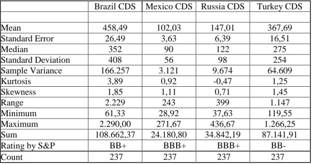
4.3.5 Sample Collection and Descriptive Statistics for Sovereign CDS Spreads ... 72
4.3.6 Implementing the Merton Model ... 82
4.4 Empirical Findings…... ... ..87
4.4.1 Granger Causality... 92
4.4.2 Principal Component Analysis ... 93
5 Conclusion ... 99
6 References ... 104
Appendix A Default Statistics for the Sovereigns ... 112
Appendix B Benchmark Bond Garch(1,1) Volatility Graphs ... 113
Appendix C Software Code for Garch(1,1) Calculation ... 115
Appendix D CDS Cumulative Distribution Graphs For Turkey in Different Maturities...116
Appendix E 5 year CDS Cumulative Distribution Graphs For the Selected Countries…….………117
Appendix F Standard Merton Model Calculation Spreadsheet Example…... 119
Appendix G Granger Causality Test Results ... 121
Appendix H Unit Root Test Results ... 129
Appendix I Cointegration Test Results ... 133
Appendix J Principal Component Analysis Results ... 141
Appendix K OLS Regression Results between the Market Rates and Model Rates for the Selected Countries………...149
Appendix L Cumulative Probabilities of the Standard Normal Distribution Function N(.)……….153
List of Figures
Figure 2.1 CDS Protection Buying Flows ... 6
Figure 2.2 Default Event ... 6
Figure 2.3 Bond Portfolio ... 8
Figure 2.4 CDS Portfolio ... 8
Figure 2.5 Asset Swap versus CDS Investment ... 9
Figure 2.6 Growth of Credit Derivatives Market ... 16
Figure 4.1 External Debt Curve Fitting: Brazil ... 75
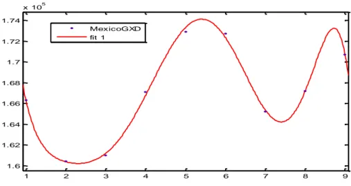
Figure 4.2 External Debt Curve Fitting: Mexico ... 75
Figure 4.3 External Debt Curve Fitting: Russia ... 76
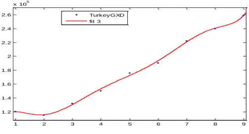
Figure 4.4 External Debt Curve Fitting: Turkey ... 76
Figure 4.5 Central Bank Reserves ... 78
Figure 4.6 CDS Graphs ... 79
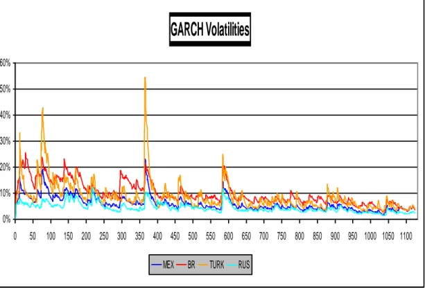
Figure 4.7 Garch(1,1) Historical Volatility Graph for the Selected Countries ... 80
Figure 4.8 Garch Correlations for the Selected Countries ... 81
Figure 4.9 Model CDS Spreads Compared to Market Observed Rates: Brazil case .. 89
Figure 4.10 Model CDS Spreads Compared to Market Observed Rates: Russia case 90 Figure 4.11 Model CDS Spreads Compared to Market Observed Rates: Mexico case90 Figure 4.12 Model CDS Spreads Compared to Market Observed Rates: Turkey case91 Figure 4.13 PCA result graph: Turkish case ... 95
Figure 4.15 PCA result graph: Brazil case ... 97 Figure 4.16 PCA result graph: Russia case ... 98
List of Tables
Table 4.1 EMBI Country Weightings ... 62 Table 4.2 Sample Sovereign CDS Descriptive Statistics ... 77 Table 4.3 Summary Table for the Correlation Matrix of Changes in Sovereign CDS Spreads Using Standard Deviation Methodology for Estimating Implied Country Volatility……….88
Table 4.4 Summary Table for the Correlation Matrix of Changes in Sovereign CDS Spreads Using Garch Methodology for Estimating Implied Country Volatility……….88
List of Abbreviations
B(t,T)=the time t price of a default-free zero-coupon bond with maturity T B= zero-coupon bond price
B= zero-coupon bond price, zero recovery (0, k)
B T = the prices of the default-free zero-coupon bonds
(0, k)
B T = the prices of the defaultable zero-coupon bonds with zero recovery CDO: Collateralized debt obligation
CDS: Credit Default Swap
(DB) Strike Price: Gross External Debt of the country
1
(0, k, k )
e T T = the value of $1 at Tk+1 if a default occurred in T Tk, k 1 F(0,T) = term structure of default-free interest rates
H(0,T) = term structure of implied hazard rates ISDA: International Swaps Dealers Association K=Tenor dates
LIBOR: London Interbank Offered Rate
N=The number of payment dates of the i th calibration security
N(d): is the cumulative probability distribution function for a standard normal variable
f
r : US treasury rate for the corresponding period
s= CDS rate
t: Time, Duration of the outstanding debt of the country TN=Maturity date of the bond
TR MARKET CDS : Turkish Market CDS rates TR MODEL CDS : Turkish Model CDS rates TRRESERVE : Turkish central bank reserves TRDEBT : Turkish gross external debt TRRF: US Treasury 5 yr rates
TRVOL : Turkish benchmark bond volatility
V : Underlying Asset, International reserves of the country t
V : the value of the assets of the firm
= expected recovery rate, recovery of par
Chapter 1
Introduction
In its guidelines to promote stability, confidence and soundness of the international financial system, the Basel Committee (2001) suggests that every market participant do their best to develop sophisticated risk models. However, still these days there is no standard approach to country risk analysis in the financial industry. For example different methods such as balanced-score cards, ratings, structural models, interest yields and yield spreads all are used to assess country risk.
Throughout the history, the defaults have occurred frequently. However, a model has not been developed for the country risk assessment. The Merton model which is a type of structural model is already being used for the corporate risk analysis.
So the objective of this study is to extend the Merton model to value the credit risk of a country by forming a hypothetical balance sheet for the country.
The main motivation of this thesis is to determine if Merton’s structural model yields reliable results when extended to determine sovereign Credit Default Swap (CDS) spreads. In the current literature, the Merton model is used to test credit default swap performance of the corporates, whereas in this thesis I propose to test its applicability to forecast the sovereign spread in emerging markets and especially on the emerging market sovereign credit spreads. In thesis corporates and sovereign be used in short for corporate firm and sovereign governments or countries. The main question in this search is that, in the absence of sovereign spreads, whether or not there are any independent variables or some combination of them that explain the credit spreads of a sovereign country.
In this case Merton model is used to see if these variables help explaining the existing spreads and how useful they are in explaining this relationship. As a result of this thesis, if a relation is found between the model output and market rates, it would imply that the parameters used in this thesis are important tools to improve a country’s
credit spread and rating in return. So, for instance increasing the central bank reserves, buying back foreign currency denominated debt and lowering external liabilities, would be some of the solutions to improve credit spreads. Lowering the credit default swap spreads would enable the country to finance its debt at lower rates, would enhance its credibility and eventually result in prosperity. Furthermore, having a lower level of implied volatility in foreign currency debt would be important besides others if this model yields meaningful results which would in return attract more investors.
In this thesis I will solely test the ability of the Merton model to reflect the reality of the market pricing. So, the main objective of this research will be to test the ability of the Merton model to predict spreads in the CDS market as an indication of the model’s strength.
In practice, the empirical evidence found by this research will assist market participants in determining if Merton’s model is useful in determining the components from which the credit risk premium is made of. In particular, I attempt to test whether the modified Merton model can be used as a forecasting tool for the credit default swap spreads. The time-varying parameters and their estimation has been one of the important topics in the literature. It has been put forward that the variation in parameters results in improved forecast performance.
Furthermore, the use of the credit risk indicators as an indicator of sovereign risk will be tested through the causality tests among the parameters and the market rates. The tests are assumed to imply a high degree of correlation between the credit risk indicators and the observed market data on spreads. Also both series are assumed to be cointegrated to have longer term co-movements. As market credit default swap spreads are treated as independent variables to be determined, the high correlation between the model rates and market rates will suggest that these indicators can be used as measures of sovereign credit risk, thus lending support to the Merton structural model which is setup in this thesis. In addition to the above mentioned analysis, principal component analysis will be done. The economic indicators will be examined in four individual country cases to determine if there is a relation with the credit spreads.
Finally, this thesis has two important implications and addresses 2 issues: central bank reserve management and debt management. On the highly debated issue of central
bank’s reserves, extended Merton model can be used to determine an optimum level of reserves or if the relationship between credit spreads and reserves is determined as an outcome, then the desired credit spread can be targeted through the central bank reserve accumulation to the specified degree. On the debt management side, extended Merton model can be used by the treasury as a decision tool to decide on debt buybacks or targeting a debt level for sustainability. The classical methods suggest that debt to GDP ratio is the indicator to watch for sustainability, however relating the debt level with a specific credit spread seems to be more realistic.
This thesis is structured as follows. In Section 2, credit derivatives market is explained in detail and the basis which causes the credit spreads to diverge from sovereign spreads is evaluated. Also in this section the standard CDS pricing models are elaborated and formulated to calculate the sovereign risk. Section 3 handles the literature review and structural models. In this section the Merton model is explained in detail. Section 4 shows how the model is extended to sovereigns. Besides these the implementation of the model is shown and the results are analyzed. Also this section discusses briefly how this approach can be used to evaluate potential policy choices, and it details further steps in the application of this approach to evaluating reserve management and debt sustainability.
Chapter 2
Credit Derivatives
Credit derivatives are contingent claims with payoffs that are linked to the credibility of a sovereign or a firm. The purpose of these instruments is to allow market participants to trade the risk associated with certain debt-related events. The conclusion that both sovereign and corporate debt is supported by similar incentives has important practical implications: Krueger’s (2002) proposal for a Sovereign Debt Restructuring Mechanism, which is modeled after Chapter 11 of the US Bankruptcy Code.
Credit derivative contracts are bilateral contracts and enable the buyer of the protection to transfer predetermined aspects of the credit risk on a specified debt obligation to the seller of the contract. The credit risk can be defined in general as the risk that the market value of a financial instrument will change. This can be as a result of a change in either the credit rating of the issuer or a result of a failure by the issuer to meet its contractual obligations which is called as a default risk.
Credit derivatives help the investors to transfer and get rid of some of the credit risk on the assets held, while retaining their market risk and taking on credit exposure to a debt issuer without necessarily acquiring the issuer's obligations. With increased credit derivatives usage, investors can acquire more diversified credit exposures for their portfolios, while traditional lenders can hedge their risk concentrations on specific names.
Credit spread on the other hand is defined as the yield difference between a risky and a risk free bond. So in order to determine CDS spreads there are two approaches; the first is looking at asset swap spreads and secondly, discounting the expected CDS premium cash flows.
Credit spread is related to the implied default probability and credit risk of the issuer. So obviously one who has to deal with credit portfolio risk and pricing of credit derivatives such as credit default swaps, should also take into consideration the implied
default probabilities. Credit derivatives enables investors to access credit markets and hedge credit portfolio risk while improving the liquidity in the market by the use of leverage. Also, besides these uses, credit derivatives enable the investors to short credit risk actively. As it can be observed from the volumes of derivatives trading in BIS statistics, as more reference entities are actively traded greater liquidity is ensured.
Instead of analyzing the credit risk through bond spreads, examining credit derivatives provides important advantages:
i) The first advantage is the higher liquidity in the credit default swaps market, ii) The product is less complex; for instance early call features are not present in credit default swaps which help to prevent distortions unlike in bond contracts,
iii) They help to boost globalization affect and result in increasing linkages; CDS contracts allow for a more direct comparison of cross country default risk. However this can also be a negative due to contagion affects.
Nevertheless, credit default swaps remain exotic and disadvantages such as the pricing issues with more complex collateralized debt obligation (CDO) type products still exist. For instance in recent times, as a result of the massive demand for yield around the world, the returns on investment grade bonds were far below the returns on equities that they now had to replace. So, the demand was met through products like CDO’s which has the low quality bond with a high rating, however this resulted in a wider spread downside affect on the US economy.
In the literature, many studies show the contagion effects in markets (Kodres and Pritsker, 2002). If Brazil goes through a crisis, the rest of the world’s credit standing will be somewhat affected but that Latin America's credit standing will be affected relatively more. In this thesis, the contagion and volatility spillover issues are not addressed directly however, the high liquidity in the credit default swap markets tend to increase the credit risks broadly.
A proper analogy for CDS’s can be established with the insurance policies on a risky asset. Buying protection on a bond insures the CDS holder against loss owing to default among a pool of eligible reference assets on that name. In the case of default, the protection holder delivers the defaulted bond to the seller and receives the par value of
Investor A: Buying $10m of protection on C for 50bp for 5 years Investor B: Selling $10m of protection on C at 50bp for 5 years
the asset. Traditionally, CDSs have been a physically settled derivative, but contracts increasingly specify the cash equivalent of this transaction. In return, the buyer pays the seller regular coupon for this protection. This payment is expressed as a notional spread in basis points and is paid quarterly in arrears over the pre-agreed-to life of the CDS contract or until a default event occurs. The flowchart of the transactions is shown in the Figure 2.1 below. In Figure 2.1, the diagram shows the case of ―investor A‖ buying protection from ―investor B‖ on ―company C‖ for five years.
Premium leg: 50bp paid quarterly in arrears for 5 years, Act/360
Protection leg: $10m notional of ref assets on company C protected
Figure 2.1 CDS Protection buying flows
In Figure 2.2 below, a default event is depicted which occurs on C and triggers the credit derivative.
Investor A delivers qualifying defaulted C
asset
Investor B pays par, i.e. $10m (less accrued interest
on premiums)
Figure 2.2 Default event
Investor A: Buying $10m of protection on C for 50bp for 5 years Investor B: Selling $10m of protection on C at 50bp for 5 years
As the CDS contracts are bilateral contracts between two parties, they can’t be broken without compensation. As a result, CDS contracts are used widely by the market participants as a hedge against the credit quality deterioration. This means that if an investor buys protection when spreads are tight, as spreads widen the value of that contract will rise. Therefore, a CDS can be used to hedge mark-to-market changes of a bond or as purely to take a credit view by itself. The investors prefer to use CDS contracts as hedging tools in their various investments.
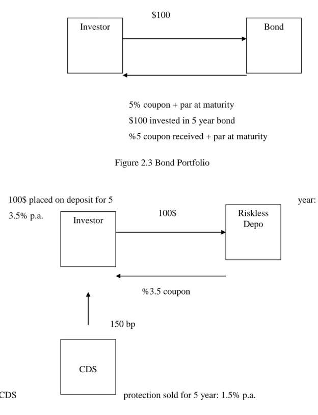
It is essential to understand the bond’s difference from a CDS contract. The underlying relationship is simple and is illustrated below by the Figure on how a CDS can be used to create a bond synthetically. As long as the reference entities are the same, the two transactions can be considered identical. So if there is a default, the investor will be exposed to same risk of holding the defaulted asset in both cases. Consider two portfolios shown in Figure 2.3 and Figure 2.4.
150 bp
%3.5 coupon $100
5% coupon + par at maturity $100 invested in 5 year bond
%5 coupon received + par at maturity
Figure 2.3 Bond Portfolio
100$ placed on deposit for 5 year:
3.5% p.a.
CDS protection sold for 5 year: 1.5% p.a.
Figure 2.4 CDS Portfolio
Investor Bond
Investor Riskless Depo
CDS
%5 coupon %3.5 coupon LIBOR
150 bp CDS Investor
So, synthetically a CDS can be created through asset swaps. The relationship between CDS’s and asset swap spreads are close apparently.
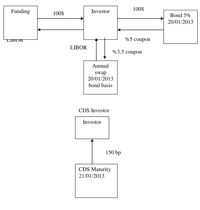
Asset Swap Investor
Figure 2.5 Asset Swap versus CDS Investment Investor Bond 5% 20/01/2013 Annual swap 20/01/2013 bond basis 100$ 100$ LIBOR Funding Investor CDS Maturity 21/01/2013
So as mentioned previously, the first method to determine CDS spreads is through asset swaps. A typical assets swap transaction is depicted in Figure 2.5. Asset swaps are related to credit default swaps because both products serve to partition credit risk. In an asset swap, an investor purchases a cash bond which is most of the times priced at par and in return for that pays the bond coupon into an interest rate swap of the same maturity. The difference between the bond coupon rate and the par swap rate is known as the asset swap spread and can be used as a hedge by the investor for the default risk on the bond.
Choudhry (2006) suggests that the possibility of arbitrage between CDS and asset swaps will eventually cause the basis to decrease between the two rates. Furthermore, he suggests that other factors might keep rates from converging.
The example in Figure 2.5 depicts that an investor with an asset swap position is in almost an identical position to one who has sold CDS protection on the same entity. In both cases the investor receives the same premium flows, even in the case of default; the investor is left with a defaulted asset. So, the asset swap spread and CDS spread should remain closely related.
2.1 The Credit Default Swap Basis and Its Importance
The credit default swap basis is important in the sense that without basis the credit default swap spread would have been equal to risk free rate plus sovereign risk premium which would have been near that sovereign’s bond yield. So when we are aiming to forecast the sovereign CDS spreads, it is indeed an endeavor to explain the variance of CDS basis. The reason for this is that CDS spreads can easily be found by adding asset swap spreads to CDS basis.
Basis trades are considered as a credit-risk-neutral method to benefit from the differences between asset swap spreads and CDS spreads. If an investor needs to hedge himself by converting from fixed rate to floating rate against falling rates, he can do so by swapping between a fixed coupon bond to a floating rate note, which means that he sells his bond at the current market price and simultaneously buys a floating rate note at par. Some factors in the market result in a difference between synthetically calculated
credit default swap rates and its price which is traded in the cash market using asset swaps. Also these differences sometimes cause arbitrage opportunities and yield to basis trading in the markets. The basis can be regarded as the difference between the credit risk premium which is reached by synthetic means and the cash market premium. The basis difference can be generalized to be positive most of the times and rarely negative. The way to represent this is;
CDS Basis = CDS spread – asset swap spread
Therefore, a negative basis is when the asset swap spread is wider than the CDS, whereas a positive basis is where the CDS is trading wider than the asset swap spread.
Buying the basis is a trade that seeks to profit from a widening of the basis. In order to long the basis, an investor buys the bond, executes a swap and buys protection on the CDS. On the other hand, selling the basis is based on the idea of profiting from a tightening of the basis. To short the basis, one must sell the bond, do an interest rate swap and buy protection on the CDS.
In terms of credit risk basis trades do not bear any risk. However, some risks such as the credit and CDS counterparty defaulting at the same time still remain which is called the joint default probability. These probabilities depending on the location and the risk that the counterparty takes in that country might be high. So when buying a Turkish CDS protection contract from a Turkish bank will carry a joint default probability risk for the CDS buyer.
Considering that the markets are assumed to be arbitrage free, it seems inconceivable that the basis should exist at all for any length of time. The reasons behind basis may be various, either market or asset specific. The factors causing this difference can be that the bond being the cheapest to deliver, the borrowing rate, expectation of a premium and the counterparty risk. Some of the reasons for the existence of basis are mentioned below briefly:
i) Supply and demand: Despite the presence of basis, it might not be possible to obtain bonds due to supply shortage or excess demand. For instance, whenever a counterparty
has a short position in a cash bond, this might result in a change in borrowing rate in the repo market from LIBOR and in this case the bond is treated as special depending on liquidity or other factors. This does not impact the default swap price which is fixed at the start of the CDS contract. This just means that as the bonds are not available at all times, the bonds can be treated special which means that they can be hard to borrow and short in the market. Therefore, even though selling the basis might sometimes look attractive, it might not be possible to realize.
ii) Calculation complexity: There might be some complexities in calculation in case of bonds trading above/below par. Whenever bonds have high coupons, they may trade above par which results in the basis trade becoming more complex. This is especially true for emerging markets where the yields and coupons are higher. A bond worth 110% will be incorrectly hedged by an equal notional amount of CDS, and the losses on the bond will be higher as the CDS contract returns par in case of default. So this is adjusted in the basis calculations by comparing Z-spread with an adjusted CDS spread, but there is no strict market convention on the topic.
iii) Increase in the volume of structured credit derivatives: When the structured credit derivatives are issued, the exposures are preferred to be hedged by selling protection into the single-name market, and mostly in large quantities. This excess supply can temporarily result in a squeeze in the spread of single names CDS’s and CDS indices. Due to the tremendous increase until this credit crunch, the average basis on many bonds has been negative due to this development.
iv) The cheapest to deliver bond: Another important factor could be that the bondholder knows the bond he is holding in the event of default; however, credit default swap sellers may receive potentially any bond from a basket of deliverable instruments that have a priority rank with the cash asset, where physical settlement is required. The CDS contracts require one reference asset to be delivered at the choice of the protection buyer. The basis exists due to the risk of a mismatch which occurs between the bond in the asset swap and the cheapest to deliver in the CDS contract.
v) The problem with funding long-term positions at Libor: Since the basis itself is relatively small, basis trades require significant amount of leverage to generate substantial return on positions. These positions need to be held for some time.
vii) Regulations: Assets are mostly held on balance sheet whereas derivatives are held off balance sheet. Due to this difference some regulations regarding the economic capital calculations as well as accounting treatment can shift investors’ preferences, resulting in a skew to the basis.
For those reasons listed above credit default swap prices often differ from the cash market prices for the same reference entity. Therefore banks are more widely using models they utilize for credit risk based on interest rate risk modeling.
CDS pricing models utilize expected cash flows and discount them in order to calculate CDS spreads as an alternative to asset swap spreads. The CDS spread is the internal rate of return value which is present value of expected premium payments.
2.2 Sovereign Risk and the Credit Derivatives Market Overview
Sovereign defaults have been observed repeatedly throughout the history of mankind. Even the industrialized countries have defaulted in the past. France and Spain constitute examples of this kind. Reinhart (2003) reports that France defaulted on its sovereign debt eight times between 1500 and 1800, while Spain defaulted thirteen times between 1500 and 1900. Conceivably, emerging market countries have defaulted more. The emerging markets frequently defaulted on their sovereign debts over the past quarter of a century.
While the concern for default risk remains, also the magnitude and complexity of the default cases have increased significantly in the last decade. When investing in the sovereign debt of a foreign country, an investor must consider two important risks. The first one is the political risk, which is the risk that even though the central government of the foreign country has the financial ability to pay its debts as they come due, for
political reasons, the sovereign entity decides to default on its payment, called the willingness to pay factor. The second type of risk is default risk, which is the same old inability to pay one’s debts as they become due.
Among these two sovereign risk types, the default risk can easily be considered the most important and the more common. The defaults are mainly caused by three factors: the value of sovereign assets, asset volatility, and leverage which is usually referred to as the debt to equity ratio. By definition whereas the determination of assets of the corporate are straightforward, for a sovereign it is more debatable. But in general, sovereign asset value is defined as the combined market value of all sovereign assets. These assets can be either cash flows generated by its trade activities or by its borrowings. Since the economic prospects for a country are not deterministic and might be highly uncertain, volatility is the only way to capture the inherent uncertainty. Leverage measures the size of the sovereign’s liabilities which are measured in book value terms since these are the amounts that the sovereign is to pay. However the leverage of a sovereign might not be too easy to determine in most cases.
The approach to sovereign risk resembles and follows a similar thinking which has been used to model corporate credit risk. However, unlike the corporate, sovereign nations can’t be liquidated and the assets can’t be transferred from the debtor to the creditor in sovereign defaults. There are debates on whether the sovereigns should choose to default which would help them to get rid of their debt burden, and use its resources for the public welfare. It is the common sense that defaulting on ones debt will temporarily boost consumption, so it is natural to raise questions about why sovereigns do not default more frequently. But obviously some costs are incurred by the default which can be in different forms of penalties imposed by external creditors on the cost of defaulters to access future finance. Also, defaulters face the risk of losing access to borrowing from financial markets. Moreover, there might be a loss of trade financing which might cause trading volume to come down. And last but not the least, given that defaulting may cause a broader financial crisis, any attempt to boost current spending temporarily through a default may not be successful.
Overall, the empirical evidence suggests that sovereign default is not necessarily associated with a loss of market access, so fears about any such loss may not in
themselves be a major deterrent to default. More generally, Gelos (2004) find that it only took defaulters three and half months, on average, to regain market access after defaulting during the 1990s compared with more than 4,5 years during the 1980s.
Although, the empirical evidence does not suggest that default necessarily closes off market access, it does point to an adverse effect on the government’s cost of future borrowing. Ozler (1993) finds that, during the relatively quiet periods of the 1970s, lenders charged up to 50 basis points more for loans to previous (post-1930) defaulters. And more recently, Reinhart (2003) find that entrepreneurial market economies with a history of defaulting on their external debts received a lower credit rating over the 1979-2000 periods than non-defaulters that displayed similar financial strength.
Argentina’s recent crisis in 2001 can be thought as an exception. Especially in the case of Argentina, the cyclical developments were more important. The abundance of a huge liquidity in financial markets helped Argentina to reach financing channels. And also an oil rich and politically driven neighbor Venezuela’s help to provide financing can’t be ignored by any means.
Respectively more important motivation for the governments may be to avoid broader losses to the domestic economy associated with default, beyond those caused by a tightening in the terms and conditions on borrowing imposed by foreign creditors.
As a consequence of the fluctuations in emerging market crises in the 1980s and 1990s, and furthermore increasing financial integration, country risk analysis has become a growing field of interest. Both for the countries itself and for international creditors besides investors, it is of crucial importance that the assessment of country risk takes place on a sound and objective basis. Easterly (2002) found that for the countries trying to re-access markets after a default, transparency and good governance are important conditions for access to international financial markets
By any benchmark, the growth of credit derivatives recently has been tremendous. The credit derivatives market has developed from being a niche to a highly liquid over the counter market within just a few years. The volumes in the market has spiked considerably as well. The popularity of credit derivative instruments can be explained by numerous factors. But all in all, they are used to protect against any possible credit event of a regular firm but largely used to protect against lower investment rated credits.
Credit Default Swaps Outstanding Amounts -5.000 10.000 15.000 20.000 25.000 30.000 35.000 40.000 45.000 50.000 55.000 60.000 65.000 70.000 1H01 2H01 1H02 2H02 1H03 2H03 1H04 2H04 1H05 2H05 1H06 2H06 1H07 2H07 Date Am o u n t ( Billion US D)
Hence these derivatives in particular have gained popularity in emerging markets which tend to be more volatile and have generally less credit-worthy private banks and corporations than do developed countries.
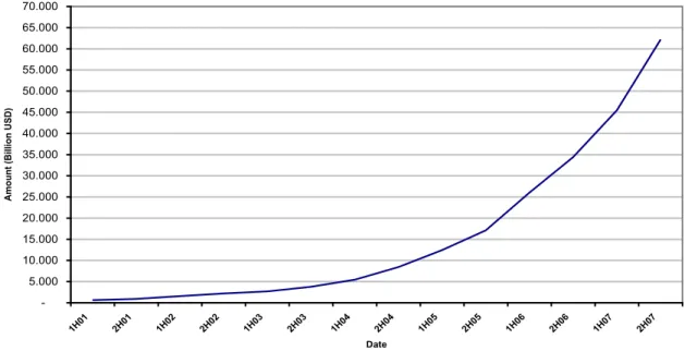
ISDA defines credit derivatives as credit default swaps referencing single names, indexes, baskets, and portfolios. By this definition, the outstanding notional CDS market reached to a volume of $62.2 trillion as of year-end 2007 according to the International Swaps Dealers Association (ISDA) which is shown below in Figure 2.6.
Figure 2.6 Growth of Credit Derivatives Market (US Dollars in Billions)
Source: ISDA Credit Derivative Market Survey
The market has been experiencing high double-digit growth since 2001, when it actually became liquid enough to track. At the start CDS’s were thought to serve loan portfolio managers to hedge out their risks, however the demand the users of CDS are from several sources, including speculators, hedgers, structured product arrangers, and arbitrageurs. The largest volume of the credit derivatives market is traded through CDS’s on a single name rather than an index CDS which are newly being developed. These contracts are used by a bondholder to protect against a default by the bond issuer. CDS’s have both a protection leg and a premium leg for a transaction. The protection
leg gives the right to a CDS holder to sell the bond at par which is essentially the same as a put option. This put option can only be exercised at the default time and in return the par value minus the recovery value is received from the protection seller. A CDS is an over the counter contract (OTC) in which the protection seller agrees to compensate for the losses on a defaulted bond. If default occurs before some fixed maturity date where the most liquid ones are mostly 5 years maturity, then the protection buyer can exercise his ―put‖ on the defaulted bond to the protection seller for par. In return for this put, the protection buyer is obliged to pay the seller a premium until the earlier of default and maturity. As defaults are unlikely to occur on quarter ends, the buyer must also pay accrued interest at the default time. Once default occurs, the premium payments are stopped and the exchange of par versus the recovery rate takes place.
There are a number of factors behind the recent huge growth rate of the CDS market such as the flexibility of credit derivatives. CDS’s also offer greater liquidity which might provide investors room for trading. Regardless of the underlying bond’s issuance size, investors can go long or short any maturity and in any currency they choose. Even in some cases the credit default swaps outstanding can be a few times of the outstanding issue size of the bond of that entity. Also Citigroup report (2007) suggests that another reason why CDS market has grown so much is that products such as interest rate swaps had already paved the way for the credit default swaps in terms of expertise. Both interest rate swaps and credit default swaps required same processes and as a result CDS’s were able to benefit from what was already in place in terms of modeling and pricing.
The growth of the CDS market has lead to various outcomes as well. Adrian, Shin (2007) found that an active CDS market has a modest beneficial effect for corporate issuers with respect to their borrowing costs. However, a more interesting conclusion of their study was that nowadays the creditors have looser lending standards than prior to pre CDS periods. This suggests that the ability to transfer the credit risk easily into the markets causes lenders to be less focused on the lending standards as these credits will be also trading in the second hand market due to increased liquidity.
One potential side-effect of derivative usage in general is that they may present some problems as investors have fewer incentives to gather information and the amount
of credit derivatives can exceed the amount of underlying securities. During high volatility periods, all the banks and investors run to hedge their risks which in turn result in higher volumes in credit default swap markets compared to other markets. So especially under these circumstances when there is a liquidity premium, the CDS markets underperform all the other instruments. On the other hand, they tend to overperform the other markets in times of positive mood as well. The amount of hedge required that would be provided by buying or selling protection is related to the hedge ratio, which is captured by the structural models.
2.3 Credit Default Swap Pricing Models
There are various models for pricing credit risk in the corporate sector. These models mostly concentrate on credit ratings, risk premiums and default rates. Caoulette (1998) suggests in his survey that these models depend on traditional actuarial methods of credit risk. Obviously there is no standard model for credit, part of the reason being that each of the models has its own set of advantages and disadvantages, making the choice of which to use depend heavily on what the model is to be used for.
Rating agencies utilize the default probabilities calculations more than other institutions. Altman(1977) has been the first to describe the techniques that can be used to forecast default probabilities.
Default might have various reasons which would range from macroeconomic factors such as high volatility in global economy, high interest rates, and recession to microeconomic factors such as poor management, high deficits due to populism by the governments and so on.
There are various causes that make default very hard to predict. In the corporate sector under these cases, default is a result of an inability to pay. In the case of sovereign debt, default may not be a result of an inability to pay, but may be due to an unwillingness to pay that is driven by political motives. Due to the mentioned factors, the literature on country risk has recognized the importance of the willingness factor. There have been many studies on the willingness to pay factor. Eaton, Gersovitz, and Stiglitz (1986), for example, argued that because a country’s wealth is always greater
than its foreign debts, the real key to default is the government’s willingness to pay. Borensztein and Pennacchi (1990) suggest that besides other observable variables that are tested, the price of sovereign debt should be related to an unobservable variable that expresses the debtor country’s willingness to pay. Clark (1991) suggests that the price of sovereign debt is related to a country’s willingness to pay which is motivated by a desire to avoid the penalties of default.
Besides the willingness to pay calculation difficulty, these models don’t also take into account the correlation among probabilities of default and estimates of possible losses. Finally, adding to the complication of credit risk modeling is that the data collected regarding default rates are not necessarily consistent with the definition of credit events for determining a payout trigger for a credit default swap. For example, data on defaults by rating agencies do not include restructuring of debt obligations. Yet, in a trade the ISDA definition of credit events may include restructuring. As a result, a debt restructuring due to a postponement of the principal repayment must be taken into account in modeling credit risk for evaluating a credit default swap but default data would not reflect such credit events.
The standard modeling framework for valuing default has the following simplifying assumptions:
1. The risk free interest rates are deterministic.
2. In the case of a default, the recovery rate is a deterministic fraction of par value. 3. Perfect capital markets are assumed: CDS contracts are assumed to be default free. 4. The default time is random and can not be predicted. The risk neutral probability of defaulting during the short time interval (t, t +e), conditioning on surviving until t, is given by l(t)e, where l(t) is assumed to be known at inception, t = 0.
The vulnerabilities in the world due to globalization have increased in the past years, and credit risk has become more important for economic policymakers. The economies can be severely damaged during a crisis period so even this highlights the need for a comprehensive framework to assess the strength of the financial systems.
The payout on a credit derivative is commonly triggered by the occurrence of a credit event - an event that affects the credit status of the reference name and these
events are defined in The International Swap Dealers Association (ISDA) definitions. These are almost standard definitions of a default in the markets.
- Moratorium - Failure to pay
- Repudiation of the debtor's obligations - Restructuring of the debt
- A credit event on other obligations of the reference name which triggers a cross-default - Accelerated repayment of the debt on the reference asset
The methodology is straight forward for a credit derivatives transaction. Like any swap, a CDS has two legs: the fixed leg which is the fee-payment leg and the floating leg which is for default insurance. The protection seller has a short position in the protection leg. As a result, the protection seller loses the difference between par and the bond’s recovery value at the default time whenever default occurs before maturity of the CDS. As the protection short position takes the risk of a default, he is compensated by receiving a premium in return for taking the risk, so protection seller is long the premium leg. The cash flows for the protection seller comprise of the fixed premium plus the accrued interest at the default time. Since CDS have no upfront premium, the CDS spread is the annualized premium payment rate that equates the initial value of the premium leg to the initial value of the protection leg.
A typical credit default swap pricing is formulated as below using the notations listed in Schoenbucher (2003);
s= CDS rate
TN=Maturity date of the bond
N=The number of payment dates of the i th calibration security K=Tenor dates
B(t,T)=the time t price of a default-free zero-coupon bond with maturity T B= zero-coupon bond price
B= zero-coupon bond price, zero recovery = expected recovery rate, recovery of par (0, k)
B T = the prices of the default-free zero-coupon bonds
(0, k)
B T = the prices of the defaultable zero-coupon bonds with zero recovery
1
(0, k, k )
e T T = the value of $1 at Tk+1 if a default occurred in T Tk, k 1
F(0,T) = term structure of default-free interest rates H(0,T) = term structure of implied hazard rates
So accordingly the fixed leg consists of the payment of n' 1s at n k T assuming no default until n k
T . The value of the fixed leg is:
' 1 1 (0, ) n N n k n s B T (2.1)
whereas the floating leg consists of the payment of recovery rate (1- ) at T , again k
assuming no default until Tk 1,T . Then the value of the fixed leg can be interpreted k
as follows: 1 1 (1 ) (0, , ) N k k k k e T T 1 1 1 (1 ) (0, , ) (0, ) N k k k k k k H T T B T (2.2)
The initial assumption made to move forward is that the market CDS spread is assumed to have the same value for the fixed and floating leg of the CDS. So with that assumption (2.1) and (2.2) can be combined to yield the market CDS rate in the model:
1 1 1 ' 1 1 (0, , ) (0, ) (1 ) (0, ) N n k k k k k k N n k n H T T B T s B T (2.3)
For the tenor dates and payment dates being equal, for instance N=K,
n
k n
T T ,
'
k k, then the CDS rate can be calculated as a weighted sum of the implied hazard rates over the life of the CDS:
1 1 (1 ) (0, , ) N n n n n s w H T T (2.4)
Equation (2.4) gives an idea over the size and dynamics of the implied hazard rates of default H(.). They should be of the same order of magnitude as a typical CDS rate divided by an expected loss rate in default, and the relative dynamics dH / H should accordingly resemble the relative dynamics d s s/ of the CDS rates in the market.
The weights of the implied hazard rates are given by;
1 1 1 (0, ) (0, ) n n n N m m m B T w n N B T (2.5)
The sum of the weights is equal to one
1 1 N n n w .
Rebonato (1998) has also calculated the result for interest-rate swap rates which resembles the equation (2.4):
' 1 1 (0, , ) N n n n n s w F T T (2.6)
1 1 1 (0, ) ' (0, ) n n n N m m m B T w n N B T
Considering that after the initial date, the value of a CDS can change, the mark-to-market value of a CDS that was originally entered as protection buyer at a CDS spread of s' is:
The Mark-to-market value = 1
1 ( ')( (0, ) ' ) n N k n n s s B T (2.7)
As s symbolizes the current CDS rate, if a short protection position is entered, the mark-to-market value should be derived from the difference between (s s which is to ') be paid over the remaining periods of the CDS. If a default occurs then the protection payments will cancel out each other, and the fee difference payment will be canceled as well. So this means that the fee difference cash flow is defaultable and must be discounted with defaultable zero-coupon bonds B(0, )T .
The important conclusion that can be derived for this thesis from these equations is that the CDS’s can be used to take exposure against spread movements. The CDS’s are used mostly for trading default probabilities instead of as investment purposes. The sensitivity of the market value of a CDS position is the main reason for this. So, not only default risks can be hedged but CDS’s can be used to trade the spreads which represents the majority of the CDS trades in the market these days. As much as default risk, the CDS market reflects liquidity conditions in the underlying bond markets and simple momentum trading. Momentum and liquidity were the main drivers of CDS prices on in the last 5 years, when the market grossly underestimated default risks; and, momentum and liquidity are the main drivers on the way up.
CDS’s instead of implying default probabilities most of the time, simply reflect the imbalance of supply and demand for protection. In a market where the liquidity dries up, the protection sellers disappear, since no bank is prepared to accept the risk of margin calls and mark-to market losses if the CDS price moves against it in the
short-term. In these cases, the protection buyers become price insensitive and are willing to pay almost any price to close out losses on the credit default swap positions which are sold at much lower prices. Then if the probability of default is tried to be measured in these types of markets, it will be observed that CDS prices have almost no relation to the probabilities of default which they supposedly imply. This logic applies to other index and composite type CDS products which are originally supposed to reveal insight about the default probabilities.
The bond yields and CDS rates are a function of the market liquidity in the underlying instruments and this relation has been increasing in the last few years. So rather than implying default, the liquidity has to be given more emphasis. The reason for this is that investors trading these assets under the current market conditions are obliged to value these assets on their collateral values and have to marked-to-market these assets. So the discounted cash flows or internal rate of return in this case is not important for the market players. For instance though unlike corporates, sovereigns default rarely, some sovereigns might imply higher default probabilities than the corporates operating in those countries. Despite the fact that the market knows that these issuers are not going to default, with the possibility of a widening of prices, the protection sellers know that prices would trigger sales due to margin call requirements. According to the efficient market hypothesis, the arbitrage opportunities created by the extreme widening of liquidity-based CDS spreads should fade away by selling the protection spreads and shorting underlying bonds or equity which is indeed selling the basis trade. This is however only possible if the investors can leverage themselves and find ways of financing these trades. Under the conditions mentioned, where the liquidity is lower, the markets are not capable of tightening the CDS spreads into alignment with underlying default probabilities. As a result of these developments, the market can be told to be distorted. First, CDS spreads decouple from the value of the underlying assets. Secondly, the bond and CDS pricing become a liquidity and momentum trading issue. So the CDS spreads should be treated as a trading tool rather than implication of default probabilities.
As mentioned above, the sensitivity of the market value of a CDS position means that CDSs are useful instruments to gain exposure against spread movements, and not
just against default arrival risks. For simplicity, in this thesis a credit event will be equated with loan default, since the main objective is to determine the relationship of the credit default swap spread with the actual market rates. However, a credit event may be defined by the parties to include any credit risk which could materially affect the market value of the reference asset as in the case of a specified ratings downgrade.
Chapter 3
Literature Review
3.1 Traditional Studies and New Attempts to Provide a Methodology for the Determination of Corporate CDS spreads
Everything being equal, a country which experiences higher volatility in its fundamentals should also experience weakening of the fundamentals, which would result in a possible default. In return, the yields on its liabilities and credit spreads will increase. This intuition has been reflected in Merton’s (1974) model of risky corporate debt, where an investor views risky debt as a combination of safe debt and a short position in a put option. The value of the option depends on the volatility of the underlying firm value; hence the value of the firm’s bonds also depends on this volatility. In the case of a sovereign, higher volatility of fundamentals increases the value of the default option and thereby the spread. Despite the importance and widespread understanding of this theory, it has been largely ignored by the empirical literature on sovereign debt, which has tended to focus exclusively on the level of variables. Two exceptions are Edwards (1984), who includes variability of reserves and finds that it is insignificant, and Westphalen (2001), who finds some limited effect of changes in local stock market volatility on changes in short term debt prices. In the corporate bond context, Campbell and Taksler (2003) find a strong empirical link between equity volatility and yield spreads.
Only a few studies to date analyze the influence of theoretical determinants of credit risk on CDS spreads. Benkert (2004) concentrates on the influence of different volatility measures on CDS premia, finding that option implied volatility has the strongest effect; Cossin et al (2002) argue that rating is the most important single source of information in the spread; Ericsson et al (2004) investigate the influence of leverage, volatility and interest rates on single-firm CDS concluding that these variables are
important determinants of CDS spreads. Other empirical studies covering the CDS market include Hull et al (2004), who compare credit risk pricing between bond and CDS markets, and found out that differences are quite small. Furthermore, their evidence suggests that CDS spreads are helpful in predicting negative rating events. Houweling and Vorst (2005) came out with the result that the reduced form models outperform bond yield spreads. They compared market prices of credit default swaps with model prices and concluded that a simple reduced form model prices credit default swaps better than comparing bonds yield spreads to CDS premiums.
The variables influencing CDS spreads in structural default models are various. For instance, the short rates are one of the factors affecting the default probability. An increase in the short rate should decrease the default probability. The theoretical argument supporting this is that the short rate influences the risk neutral drift in the firm value process: a higher short rate raises the risk neutral drift and lowers the probability of default. Besides the short term rates, the slope of the yield curve is considered important. The steeper the yield curve, the higher the expected future short rate and thus we expect a negative relationship between both the short rate and the slope of the yield curve and the CDS spread. Low interest rates are often observed during periods of recession and frequent corporate defaults. In addition the steepness of the yield curve is an indicator of an increase in future economic activity. Fama (1984) and Estrella and Hardouvelis (1991)’s work support this idea.
Default data are considerably less in comparison to the data available for the modeling of interest rate risk. It is rather difficult to form time series of defaults whereas Treasury prices are available to every individual on a daily basis for many decades.
Longstaff (2003) argues that the bond market is lagging the derivatives market in terms of price discovery. However, a bias is present in the econometric results of this study since the potential cointegration relationship across the markets is ignored.
In the light of these and other pragmatic considerations, studies of sovereign debt pricing have focused primarily on models based on the intensity processes that have been exogenously specified. Merrick (1999) has studied Russian and Argentinian bonds and has calibrated a discrete-time model to these bonds which utilize models with a
constant intensity. Keswani (1999) and Pages (2000) have studied and implemented special cases of the modeling framework of Duffie and Singleton (1999) to data on Latin American Brady bonds. Dullmann and Windfuhr (2000) apply a similar framework to pricing European government credit spreads under the European Monetary Union. Implicit in these formulations are the assumptions that holders of sovereign debt face a single credit event default, with liquidation upon default and that the bonds issued by a given sovereign are homogeneous with regard to their credit characteristics.
There are few studies in the literature regarding the defaultable bonds and several models have been proposed for this purpose. (Duffie and Singleton (2003)) lists three main approaches:
i) Merton’s (1974) option pricing based model, which computes the payoff at maturity as the face value of the defaultable bond minus the value of a put option on the issuer’s value with an exercise price equal to the face value of the bond.
ii) Structural models, which are the followers of the Merton model relax one of the unrealistic assumptions of Merton’s model that default occurs only at maturity of the debt, when the issuer’s assets are no longer sufficient to face its obligations towards bondholders. On the contrary, these models assume that default may occur at any time between issuance and maturity of the debt and that default is triggered when the issuer’s assets reach a lower threshold level (Black and Cox (1976) and Longstaff and Schwartz (1995)).
iii) Reduced-form models, which do not condition default explicitly on issuer’s value, and therefore are, in general, easier to implement. These models are different than structural models in the sense that they approach in a different way to defaults. The degree of predictability of default differs, as the reduced form models which are developed by Jarrow, Lando and Turnbull (1997) and Duffie and Singleton (1999)) accommodate defaults coming as sudden surprises.
Structural models like the Merton model, assume that the modeler has the same information set as the officials- complete knowledge of all the assets and liabilities. Due
to this assumption regarding the symmetry of information, the default time is assumed to be predicted in advance. For cases where an issuer’s outstanding bond amount is too large in the market, reduced form models are expected to do better. However, for the structural models, Merton model is rather useful but has simplifying assumptions; and appropriate modifications to the framework are necessary.
Making more deterministic assumptions is clearly not possible to realize. If the assumptions lead to predictions that are good enough by making plausible and enough realistic assumptions, that would be the most desired and optimized outcome.
This insight presented applies to the current debate regarding structural and reduced-form models. While much of the debate rages about assumption and the underlying theory, relatively little work is done about the empirical applicability of these models. The research result obtained by this thesis is expected to improve the understanding of the empirical performance of several widely known credit pricing models.
For corporate credit spread calculations, there are a few practical methods developed in the market by using Merton model. Two of those approaches will be mentioned here briefly. These methodologies are called CreditMetrics and KMV models. These models rely on the firm value or so called asset value model which are originally proposed by Merton (1974). However, their implementation has quite different features and assumptions. These models differ quite substantially in the simplifying assumptions they require in order to facilitate its implementation. In fact, the framework to analyze credit risk calls for the full integration of market risk and credit risk. Yet there are no models satisfying this criterion and reached the sophistication.
The first of these models is CreditMetrics. CreditMetrics is developed by JP Morgan, first published and well publicized in 1997. The CreditMetrics approach is based on credit migration analysis which is based on the probability of moving from one credit quality to another, including default, within a given time horizon, which is often taken arbitrarily as 1 year. CreditMetrics models the full forward distribution of the values of any portfolio where the changes in values are related to credit migration. In this case the interest rates are assumed to evolve in a deterministic fashion. Credit value
at risk of a portfolio is derived in the same methods as for market risk. It is simply the percentile of the distribution corresponding to the desired confidence level.
The second model is the KMV model which is developed by a firm specialized in credit risk analysis. KMV Corporation has developed a credit risk methodology over the last few years, as well as an extensive database, to assess default probabilities and the loss distribution related to both default and migration risks. KMVs methodology differs somewhat from CreditMetrics as it relies upon the ``Expected Default Frequency'', or EDF, for each issuer, rather than upon the average historical transition frequencies produced by the rating agencies, for each credit class.
From the actual comparison of these models on various benchmark portfolios, it seems that any of them can be considered as a reasonable internal model to measure credit risk, for straight bonds and loans without option features. All these models have in common that they assume deterministic interest rates and exposures. While, these models are convenient for simple vanilla bonds and loans, they are inappropriate to measure credit risk for swaps and other derivative products.
In order to measure credit risk of derivative securities, the next generation of credit models should allow at least for stochastic interest rates, and possibly default and migration probabilities which depend on the state of the economy. For instance the policy measures such as reserves, debt and even other factors like the level of interest rates and the stock market should also be taken into account if possible.
The insights of Black Scholes (1973) and Merton (1974) have changed the credit pricing methodology and understanding. By suggesting that these types of models systematically underestimate observed spreads, Jones (1984) has opposed to these structural models of default. His research reflected a sample of firms with simple capital structures observed during the period 1977-1981. Ogden (1987) confirmed this result, finding that the Merton model under predicted spreads over US Treasury securities by an average of 104 basis points. Moody’s KMV revived the practical applicability of structural models by implementing a modified structural model called the Vasicek-Kealhofer (VK) model (Vasicek, 1984; Crosbie and Bohn, 2003; Vasicek-Kealhofer, 2003). Black and Cox (1976) treat the point at which the default occurs as an absorbing barrier. Geske (1977) on the other hand deals with the liabilities and solves the liability claims