Development of a non-ordinary state-based peridynamics solver

DEVELOPMENT OF A NON-ORDINARY

STATE-BASED PERIDYNAMICS SOLVER

a thesis submitted to

the graduate school of engineering and science

of bilkent university

in partial fulfillment of the requirements for

the degree of

master of science

in

mechanical engineering

By

Rico Morasata

September 2019

DEVELOPMENT OF A NON-ORDINARY STATE-BASED PERI-DYNAMICS SOLVER

By Rico Morasata September 2019

We certify that we have read this thesis and that in our opinion it is fully adequate, in scope and in quality, as a thesis for the degree of Master of Science.

Ali Javili(Advisor)

Onur Özcan

Ercan Gürses

Approved for the Graduate School of Engineering and Science:

Ezhan Karaşan

ABSTRACT

DEVELOPMENT OF A NON-ORDINARY STATE-BASED

PERIDYNAMICS SOLVER

Rico Morasata

M.S. in Mechanical Engineering Advisor: Ali Javili

September 2019

Damage prediction is crucial in the design process of engineering structures to ensure struc-tural integrity. The limitations of empirical methods and the high costs associated with experimental analyses have prompted the development of numerical methods to predict the initiation and/or propagation of cracks under prescribed loading conditions. While various methods exist for failure prediction, their formulations rely on partial differential equations with spatial derivatives. As a result, these methods require special treatments in order to accurately capture the underlying failure mechanisms. To overcome these limitations, the peridynamic theory has been introduced as a novel, nonlocal continuum formulation. In contrast to the other methods, it is expressed as an integro-differential equation devoid of spatial derivatives, hence applicable to structural analyses involving discontinuities. This project aims to elaborate on the development of a solver based on a specific variant of the peridynamic formulation to investigate the behavior of two- and three-dimensional structures under certain loading conditions. The current code is developed to solve quasi-static prob-lems related to damage initiation and propagation. In addition, it is aimed to show that peridynamics can capture local, hyperelastic deformations. The overall structure of the code is reviewed and the potential extensions of the current work are discussed.

ÖZET

TİPİK OLMAYAN DURUM BAZLI PERİDİNAMİK YÖNTEMİ

ÇÖZÜCÜSÜNÜN GELİŞTİRİLMESİ

Rico Morasata

Makine Mühendisliği, Yüksek Lisans Tez Danışmanı: Ali Javili

Eylül 2019

Hasar tahmini mühendislik yapılarının tasarım sürecinde yapısal bütünlüğü sağlamak için kritiktir. Ampirik yöntemlerin sınırlamaları ve deneylerin yüksek maliyetleri yüzünden, çat-lakların başlatması ve/veya yayılmasını verilen yükleme koşulların altında tahmin edebilmek için, sayısal yöntemlerin geliştirmesi teşvik edilmiştir. Hasar tahmini için çeşitli yöntem-ler mevcut olmasına rağmen, onların formülasyonları gerilme tensörün bileşenyöntem-lerin türev-leri ile kısmi diferansiyel denklemlere dayanır. Bu sınırlamaları atlatmak için, peridinamik teorisi yeni yerel olmayan bir denklem olarak tanıtılmıştır. Diğer yöntemlerin aksine, ger-ilme tensörün bileşenlerin türevlerini içermeyen bir integro-diferansiyel denklem olarak ifade edilmiştir. Bu yüzden süreksizlikler içeren yapısal analizlere uygulanabilir. Bu projenin amacı iki ve üç boyutlu yapıların öngörülen yükleme koşulları altında davranışlarını araştır-mak için, peridinamik yöntemin spesifik bir çeşitine dayanan bir çözücünün geliştirilmesini açıklamaktır. Mevcut kod hasar başlatması ve yayılması ile ilgili statik problemleri çözmek için geliştirilmiştir. Ve, mevcut yöntemin yerel deformasyonların yakalabileceği gösterilmiştir. Kodun genel yapısı gözden geçilir ve mevcut çalışmanın potansiyel uzantıları tartışılmıştır.

Anahtar sözcükler: Hasar tahmini, Peridynamics, Çatlaklar, Nonlocal Continuum

Acknowledgement

First, I would like to express my deepest gratitude to Dr. Ali Javili for the opportunity to work on Peridynamics, his guidance, support and patience throughout my research. Working on Peridynamics has stimulated my interest in Computational Solid Mechanics, especially Multiscale Modeling.

Furthermore, I would like to address my special thanks to Dr. Erkan Oterkus at the Univer-sity of Strathclyde for the numerous discussions we had regarding the peridynamic theory and the associated computational procedures.

Moreover, I am highly indebted to Dr. David Littlewood at Sandia National Laboratories for his valuable insight into the crucial components of a peridynamics solver, to Dr. Patrick Diehl of the Center for Computation & Technology at the Louisiana State University for his valuable guidance and to Mr. Michael Brothers at FutureWei Technologies for his insight into the implicit time integration in peridynamics.

Also, I would like to thank Dr. Cevdet Aykanat of the Computer Engineering Department at Bilkent University for his suggestions regarding the choice of algorithms and data structures which are central to the solver development.

I would like to acknowledge my friends at the Graduate Student Office for the moments we shared. Specifically, I am thankful to Mr. Onur Vardar for our frequent discussions regarding object-oriented programming, libraries and sparse matrix operations.

Last but not least, my deepest gratitude goes out to my parents, Léontine and Jacquot, and my brothers, Teddy and Kevin, for their lifelong, consistent support; I would not have reached this far without their encouragement.

Contents

1 Introduction 1

1.1 Fracture Mechanics Overview . . . 1

1.2 Aspects of the Peridynamics Theory . . . 2

1.3 Motivation . . . 3

1.4 Research Objectives and Outline . . . 4

2 Theoretical Background 6 2.1 Fundamental Concepts . . . 6 2.2 Governing Equation . . . 7 2.2.1 Bond-based formulation . . . 7 2.2.2 State-based formulation . . . 13 2.3 Influence Function . . . 17

2.4 Zero-Energy Modes Control . . . 17

2.5 Boundary Conditions . . . 19

2.6 Correction Procedures . . . 20

2.6.1 Volume correction . . . 20

2.6.2 Surface correction . . . 20

3 Material and Damage Models 22 3.1 Constitutive Model . . . 22

3.2 Damage Models . . . 24

4 Numerical Implementation 26 4.1 Discretization of Equations . . . 26

4.2 Internal Force Density Computation . . . 27

4.3 Tangent Stiffness Matrix Approximation . . . 27

CONTENTS vii

4.5 Solver Design . . . 30 4.5.1 Neighbor search . . . 30 4.5.2 Representations of sparse matrices . . . 31

5 Discussion and Conclusion 34

5.1 Discussion . . . 34 5.2 Concluding Remarks . . . 37 5.3 Outlook . . . 37

List of Figures

2.1 Comparison of MD, CCM and PD. . . 6

2.2 Kinematics of a peridynamic continuum. . . 7

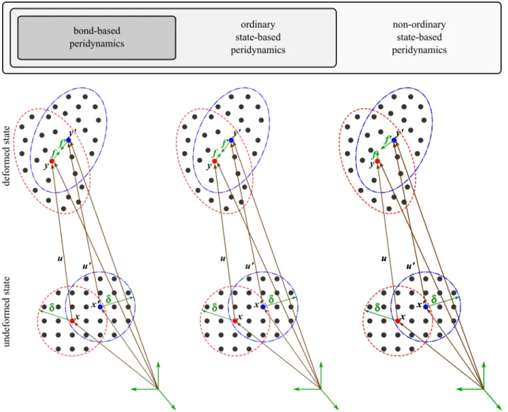
2.3 Illustration of the BB-PD, OSB-PD and NOSB-PD formulations. . . 14

2.4 Application of boundary conditions in PD. . . 19

2.5 Illustration of full and partial volumes within a neighborhood. . . 20

2.6 Material points’ neighborhoods near free surfaces and interfaces. . . 21

5.1 Cube under tension . . . 36

List of Tables

2.1 Material parameters evaluation in BB-PD. . . 12

2.2 Comparison of balance laws between PD and CCM. . . 16

Nomenclature

Abbreviations

Symbol Description

BB-PD Bond-Based Peridynamics

BC Boundary Condition

CCM Classical Continuum Mechanics

CSR Compressed Sparse Row

DBC Dirichlet Boundary Condition

DOF Degree Of Freedom

FEM Finite Element Method

IFD Internal Force Density

LEFM Linear Elastic Fracture Mechanics

LPS Linear Peridynamic Solid

NOSB-PD Non-Ordinary State-Based Peridynamics

OSB-PD Ordinary State-Based Peridynamics

PD Peridynamics

Nomenclature xi

SB-PD State-Based Peridynamics

SED Strain Energy Density

TSM Tangent Stiffness Matrix

XFEM eXtended Finite Element Method

Symbols

Symbol Description Unit

α thermal expansion coefficient K−1

∆ nodal spacing (uniform discretization) m

δ horizon m

κ bulk modulus N/m2

λ , µ Lamé constants N/m2

µ history-dependent, scalar-valued function

ω influence function

ρ density kg/m3

θ dilatation

M unit vector state in OSB-PD

T force vector state N/m6

t scalar force state in OSB-PD N/m6

X initial deformation state of x m

Y current deformation state of x m

Nomenclature xii

c bond constant in BB-PD N/m6

Gc critical energy release rate J/m2

m horizon-to-grid-spacing ratio

s bond stretch

sc critical stretch

η relative displacement vector m

σ Cauchy stress tensor N/m2

ξ peridynamic bond m

C micromodulus tensor

E Green-Lagrange strain tensor

F approximate deformation gradient tensor

I second-order identity tensor

K shape tensor

P Piola stress tensor

u′ displacement of x′ m

u displacement of x m

x′ position of a neighbor of x in the reference

con-figuration/a neighbor of x

m

x material point (its position in the reference

con-figuration)

m

y′ position of x′ in the current configuration m

Nomenclature xiii

B continuum body

Chapter 1

Introduction

1.1

Fracture Mechanics Overview

Prediction of material damage and failure by means of numerical simulations remains a chal-lenge in Computational Mechanics. Numerical methods for structural analysis are essentially based on the governing equations of Classical Continuum Mechanics (CCM) which are par-tial differenpar-tial equations with spapar-tial derivatives. As a result, difficulties emerge when the physical body under consideration contains discontinuities such as cracks. Inglis [1] proposed empirical relations to evaluate the stress concentrations in the vicinity elliptical holes using the linear elasticity theory. Since the latter assumes a continuous displacement field, these re-lations yield non-physical stress values at sharp crack tips. Aware of these results, Griffith [2] introduced an energy-based approach to predict fracture strength in brittle materials. His pioneering works laid the foundation of Linear Elastic Fracture Mechanics (LEFM). As noted in [3], LEFM is only applicable if the body under consideration has a pre-existing crack. Fur-thermore, crack growth requires the definition of external criteria. The application of LEFM into the Finite Element Method (FEM) necessitates special treatments such as remeshing the body after an incremental crack growth, so that the crack lies on element boundaries. In addition, the crack growth is defined a priori by means of a mathematical relation. These requirements affect the adequacy of the traditional FEM for practical applications involving cracks.

Various techniques have been developed to address these shortcomings including the cohesive zone concept [4, 5, 6], then the cohesive zone model (CZM) [7] as well the eXtended Finite Element Method (XFEM) [8] which is based on the concept of partition of unity method [9]. Nonetheless, these techniques have drawbacks: for the CZM, mesh quality significantly affects crack propagation and remeshing the body is necessary [10]. Although the XFEM allows for crack propagation across elements, it was observed that the method yields inaccurate solutions for problems involving complex crack interactions due to partial element enrichment around the crack tip [11]. Eringen [12] noted that the CCM formulation does not possess an internal length scale parameter that enables multiscale modeling. In contrast, due to the drastic differences in the associated length and time scales, Molecular Dynamics (MD) simulations are impractical for real-world problems at the macroscale. Consequently, nonlocal continuum theories have been introduced to account for long-range effects [13].

As indicated in [3], despite their ability to capture phenomena across different length scales, nonlocality in nonlocal theories is accounted for by means of strain averaging, i.e., their formulations still involve spatial derivatives, which is problematic when discontinuities are present in the domain.

To circumvent the difficulties associated with the aforementioned theories, Silling [14] in-troduced peridynamics as a novel continuum formulation, mathematically expressed as an integro-differential equation without spatial derivatives.

1.2

Aspects of the Peridynamics Theory

The first peridynamics (PD) formulation is referred to as bond-based peridynamics (BB-PD). Its fundamental assumption is that a continuum body is subdivided into infinitely many points of finite volume called material points, each of which interacts with those within its neighborhood through pairwise interactions of equal magnitude. As a result, several restric-tions are imposed on material properties [3]. As a remedy, an improved version of the PD formulation called state-based peridynamics (SB-PD) has been introduced [15]. There are two main types of SB-PD formulations: ordinary state-based peridynamics (OSB-PD) and

non-ordinary state-based peridynamics (NOSB-PD) formulations. In the OSB-PD formulation,

the forces between the material points act along the same line of action but are of unequal magnitudes. In contrast, in the NOSB-PD formulation, the forces have different magnitudes and can act in arbitrary directions. Therefore, the NOSB-PD formulation encompasses the

BB-PD and OSB-PD formulations and is the main focus of the current work. Since its in-troduction, PD has been attractive to researchers across a plethora of disciplines. Recently, Javili et al. [16] identified the main applications of PD up to date in various domains. Upon examining the literature, it is noted that the main applications of PD are problems involving damage and failure prediction. These analyses are generally carried out using the BB-PD or the OSB-PD formulations. Notably, Liu et al. [17] developed a highly parallel, three-dimensional BB-PD code to simulate the behavior of ductile and brittle materials. Hu et al. [18] developed a BB-PD model to investigate progressive damage in composite laminates. Oterkus et al. [19] incorporated heat conduction within the OSB-PD framework and analyzed the deformation of pre-cracked structures subjected to thermal and mechanical loads. It is worth mentioning that multiple material behaviors have been simulated by incorporat-ing classical continuum models into the NOSB-PD formulation. In particular, Warren et al. [20] implemented an isotropic elastic–plastic linear hardening constitutive model to ana-lyze three-dimensional structural deformations under transient dynamics. Foster et al. [21] extended their work and implemented a viscoplastic constitutive model within the peridy-namic framework. Furthermore, the Johnson-Cook plasticity model has been incorporated into the NOSB-PD formulation in [22], then in the work of Amani et al. [23] in the context of thermoplastic fracture. Recently, Lai et al. [24] used the modified Johnson-Holmquist material model to analyze impact-induced fracture in quasi-brittle materials.

1.3

Motivation

Given the importance of damage prediction in structural design and the costs associated with experimental procedures, tremendous efforts have been dedicated to the development of robust and accurate numerical methods.

Recently, it is noted that there has been a growing interest in meshless methods for compu-tational mechanics problems due to their flexibility in handling problems with large deforma-tions and evolving discontinuities [25]. In contrast to the FEM which requires nodal connec-tivity, the discretization does not require an underlying structure but consists of nodes only; hence they are not affected by mesh distortion, mesh reconstruction and the challenges asso-ciated with the discretization of three-dimensional geometries [26, 25]. Among the most com-mon meshless methods are the Smoothed Particle Hydrodynamics, the Reproducing Kernel Particle Method, the element-free Galerkin method and the Meshless Local Petrov-Galerkin

method. In the literature, applications of meshless methods to solid mechanics problems include metal forming [27, 28], hyperelastic deformations [29], fracture modeling [30, 31]. Marder [32] reviewed the analytical theories and numerical simulations associated with the use of particle methods in fracture modeling. PD is described as “one of the first and cer-tainly the best-developed particle method in which the particles are not atoms”. Indeed, PD has been successfully applied to a wide range of problems as shown in [16]. Further-more, significant advances have been made in the numerical implementation of PD. The earliest contribution regarding the numerical implementation of PD is the code called EMU developed by Silling [33]. It is noted that Parks et al. [34] implemented PD within the MD code LAMMPS [35]. Macek and Silling [36] implemented the discretized BB-PD within the ABAQUS commercial finite element (FE) code. The authors emphasized the importance of a PD-FE coupling for damage prediction problems in terms of computational efficiency. To date, the most effective numerical implementation of PD is the open-source, massively parallel code Peridigm [37], developed by Sandia National Laboratories. It implements the OSB-PD and NOSB-PD formulations and has been used in numerous problems involving pro-gressive damage, high-velocity impact and fragmentation. Also, the code may be extended to include custom constitutive models. Despite its remarkable features, the available documen-tation on user-defined material models is limited and the potential definition of user-defined damage models has not been indicated. The possibility to incorporate material models from CCM into the NOSB-PD formulation is highly advantageous for more realistic simulations of structural behaviors. The aforementioned contributions have motivated the present work in developing a computational framework for the qualitative and quantitative predictions of material damage and failure as well as hyperelastic deformations under prescribed loading conditions. The code is written following an object-oriented design approach.

1.4

Research Objectives and Outline

The main purpose of this project is to develop an object-oriented, extensible structural solver for the analysis of elastic deformations under various loading conditions. The code develop-ment aims to:

• provide a deeper insight into the NOSB-PD formulation, • elaborate on all aspects of its numerical implementation,

• highlight the solver’s potentials for material modeling and coupling strategies.

This manuscript is organized as follows: Chapter 2 provides a detailed description of the major peridynamic formulations. Chapter 3 elaborates on the material and damage models considered herein. Chapter 4 discusses the different aspects of the numerical implementation, particularly the discretization of equations, the construction of the tangent stiffness matrix and integration schemes. Also, it expounds on elements of the solver design namely the neighbor search and the matrix assembly technique. Finally, Chapter 5 provides an overview of the code and highlights the potential extensions of the current project.

Chapter 2

Theoretical Background

2.1

Fundamental Concepts

PD is a continuum mechanics theory in which the physical body is subdivided into material

points of finite volume. As a result, PD is, to some extent, similar to MD. MD deals with

discrete entities, i.e., atoms and molecules, at the nano- or microscale. The mutual inter-actions between these particles are governed by the parameter known as cutoff radius δ. In CCM, the state of a point within a body B is influenced by its immediate neighbors only. Therefore, the concept of nonlocality does not arise. In contrast, in PD, each material point within the continuum body _{B interacts with its neighbors located within a neighborhood H}x delimited by the horizon δ.

2.2

Governing Equation

2.2.1

Bond-based formulation

The peridynamic theory has been introduced in terms of the BB-PD formulation.

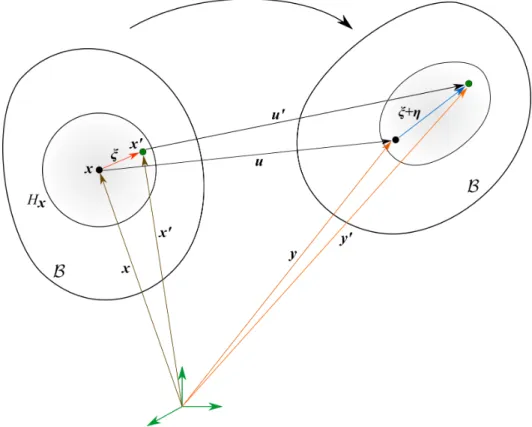
Figure 2.2: Kinematics of a peridynamic continuum.

For material points x and x′ in the reference configuration with x′ in the neighborhood of

x, let y and y′ denote their respective position vector in the current configuration. Let u and u′ denote their respective displacements. The following quantities are defined

ξ = x′− x , (2.1) η = u′ − u , (2.2) y = x + u , (2.3) y′− y = ξ + η , (2.4) s = |ξ + η| − |ξ| |ξ| , (2.5)

s the bond stretch. An alternative representation of the peridynamic formulation has been

introduced in [38] based on CCM kinematics.

The governing equation in the BB-PD formulation is

ρ ¨u(x, t) =

∫

H

f (η, ξ) dVx′+ b(x, t) , (2.6)

where ρ is the density of material point x, ¨u its acceleration, f a vector-valued pairwise force

function of unit N/m6_{, H the neighborhood and b the prescribed body force density of unit} N/m3. The pairwise force function is such that

f (−η, −ξ) = −f(η, ξ) ∀η, ξ , (2.7)

(η + ξ)× f(η, ξ) = 0 ∀η, ξ , (2.8)

where Eq. (2.7) is a restriction due to the Newton’s third law of motion and Eq. (2.8) is the conservation of angular momentum [14].

A microelastic material [39] is a material for which there exists a scalar micropotential

func-tion w such that

f (η, ξ) = ∂w

∂η(η, ξ) (2.9)

It is indicated that for a microelastic material, the two material points of a bond are “con-nected by a (possibly nonlinear) spring”. Furthermore, the micropotential function w is such that

ˆ

w(y, ξ) = w(η, ξ) ∀η, ξ (2.10)

The pairwise force function in Eq. (2.6) is of the form

f (η, ξ) = ξ + η

|ξ + η|f (|ξ + η|, ξ) ∀η, ξ (2.11) f (|ξ + η|, ξ) = ∂ ˆw

∂(|ξ + η|) (|ξ + η|, ξ) ∀η, ξ (2.12)

Within the context of small deformations, Silling [14] defined the linearization of f (η, ξ) as

f (η, ξ) = C(ξ) η ∀η, ξ , C(ξ) = ∂f

where C(ξ) is defined as the micromodulus tensor.

The material properties for the BB-PD formulation have been derived by Madenci and Oterkus [3] and will be succinctly presented herein: For the BB-PD formulation, account-ing for the pairwise interaction between material points, the force density vector t can be expressed as t(η, ξ, t) = 1 2f (η, ξ, t) = 1 2C ξ + η |ξ + η|, (2.14) t(−η, −ξ, t) = −1 2f (η, ξ, t) =− 1 2C ξ + η |ξ + η|, (2.15)

where C is a parameter dependent on material constants.

Let xk denote a material point in the reference configuration, xj a material point in the

neighborhood of xk and tkj the force density vector exerted by xj on xk. Using Eq. (2.1)

through (2.5), the peridynamic strain energy density at xk is given by Wk = a θ2k− a2θk∆Tk+ a3(∆Tk)2 + b N ∑ j=1 wkj((|yj− yk| − |xj− xk|) − α ∆Tk|xj − xk|)2Vj, (2.16)

where a, a2, a3, b are material parameters, θk the dilatation, α the thermal expansion

coeffi-cient, Vj the volume of material point xj, N the total number of neighbors of xk and ∆Tkthe

temperature change at xk. wkj will be referred to as the influence function, a dimensionless

parameter in SB-PD. The dilatation is defined as

θk = d N ∑ j=1 wkj(skj − α ∆Tk) y_j− yk |yj− yk| · (xj − xk) Vj + 3 α ∆Tk, (2.17)

where d is a parameter such that θk is dimensionless and skj is the stretch of the bond

connecting xj and xk .

The force density vector tkj is

tkj = 1 Vj ∂Wk ∂(|yj − yk|) y_j − yk |yj − yk| (2.18)

Plugging Eq. (2.17) into Eq. (2.16) and using Eq. (2.18), tkj is obtained as tkj(uj − uk, xj − xk, t) = 1 2A y_j− yk |yj− yk|, (2.19) where A = 4 wkj { d yj− yk |yj− yk| · xj − xk |xj − xk|(a θk− 1 2a2∆Tk) + b ((|yj − yk| − |xj − xk|) −α ∆Tk|xj − xk|)} (2.20) Similarly tjk(uk− uj, xk− xj, t) =− 1 2B y_j− yk |yj− yk|, (2.21) where B = 4 wjk { d yk− yj |yk− yj| · xk− xj |xk− xj|(a θj − 1 2a2∆Tj) +b ((|yk− yj| − |xk− xj|) − α ∆Tj|xk− xj|)} (2.22)

Since tjk and tkj have equal magnitude, A = B. Therefore

ad = 0 (2.23)

As a result

C = 4 b wkj((|yj− yk| − |xj− xk|) − α ∆Tk|xj − xk|) (2.24)

Inserting Eq. (2.24) into Eq. (2.14) yields

f (uj − uk, xj − xk, t) = 4 b wkj|xj− xk| (skj− α ∆Tk)

y_j − yk

|yj − yk|, (2.25)

which may be written as

f (uj− uk, xj − xk, t) = c (skj − α ∆Tkj)

y_j − yk

|yj − yk|, (2.26)

From dimensional analysis on Wk, it can be established that c

b = 4δ , (2.27)

The constraint arises from the explicit form of the influence function

wkj = δ

|ξ| (2.28)

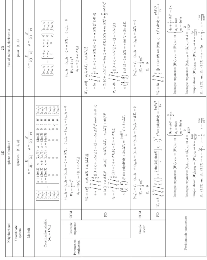
The peridynamic material parameters are determined using simplifying assumptions on the structure’s dimensions and by evaluating the strain energy density in Eq. (2.16) from a CCM standpoint. The analysis is carried out considering simple loading cases, specifically isotropic

3D 2D Neigh b orho o d sphere of radius δ disk of radius δ , thic kness h Co ordinate _system spherical (ξ , θ , ϕ ) p olar (ξ , ϕ ) Mo duli κ = E 3(1 − 2 ν ) , µ = E 2(1 + ν ) κ = E 2(1 − ν ) , µ = E 2(1 + ν ) Constitutiv e relation (σ k = C εk )  (σ        xx )k (σ y y )k (σ z z )k (σ y z )k (σ xz )k (σ xy )k        =  κ        + (4 µ/ 3) κ − (2 µ/ 3) κ − (2 µ/ 3) 0 0 0 κ − (2 µ/ 3) κ + (4 µ/ 3) κ − (2 µ/ 3) 0 0 0 κ − (2 µ/ 3) κ − (2 µ/ 3) κ + (4 µ/ 3) 0 0 0 0 0 0 µ 0 0 0 0 0 0 µ 0 0 0 0 0 0 µ          (ε        xx )k (ε y y )k (ε z z )k (γ y z )k (γ xz )k (γ xy )k          (σ  xx )k (σ y y )k (σ xy )k  =  κ  + µ κ − µ 0 κ − µ κ + µ 0 0 0 µ    (ε  xx )k (ε y y )k (γ xy )k   P arameters _evaluation Isotropic _expansion CCM (ε xx )k = (ε y y )k = (ε z z )k = ζ + α ∆ Tk , (γ xy )k = (γ xz )k = (γ y z )k = 0 W k = 9 κ 2 ζ 2 θk = tr (ε k ) = 3 (ζ + α ∆ Tk ) (ε xx )k = (εy y )k = ζ + α ∆ Tk , (γ xy )k = 0 W k = 2 κ ζ 2 θk = 2 (ζ + α ∆ Tk ) PD W k = a θ 2−k a2 θk ∆ Tk + a3 (∆ Tk ) 2 k + b δ ∫ 0 2 π ∫ 0 π ∫ 0 δ ([ ξ (1 + ζ + α ∆ Tk ) ξ − ξ ]− α ∆ Tk ξ ) 2ξ 2sin ϕ d ϕ d θ d ξ = 3 a (ζ + α ∆ Tk ) 2− 3 a2 (ζ + α ∆ Tk ) ∆ Tk + a3 ∆ T 2 k + π bζ 2δ 5 θk = d δ ∫ 0 2 π ∫ 0 π ∫ 0 δ ([ ξ (1 + ζ + α ∆ Tk ) ξ − ξ ]− α ∆ Tk ξ ) × ( ξ ξ · ξ ξ ) ξ 2sin ϕ d ϕ d θ d ξ + 3 α ∆ Tk = 4 π dδ 4 3 ζ + 3 α ∆ Tk W k = a θ 2−k a2 θk ∆ Tk + a3 (∆ Tk ) 2 k + bh δ ∫ 0 2 π ∫ 0 δ ([ ξ (1 + ζ + α ∆ Tk ) ξ − ξ ]− α ∆ Tk ξ ) 2ξ d θ d ξ = 2 a (ζ + α ∆ Tk ) 2− 2 a2 (ζ + α ∆ Tk ) ∆ Tk + a3 ∆ T 2 k + 2 π 3 bhδ 4ζ 2 θk = dh δ ∫ 0 2 π ∫ 0 δ ([ ξ (1 + ζ + α ∆ Tk ) ξ − ξ ]− α ∆ Tk ξ ) × ( ξ ξ · ξ ξ ) ξ d θ d ξ + 2 α ∆ Tk = π dhδ 3ζ + 2 α ∆ Tk Simple shear CCM (γ xy )k = ζ , (ε xx )k = (ε y y )k = (ε z z )k = (γ xz )k = (γ y z )k = ∆ Tk = 0 W k = 1 µ 2 ζ 2 θk = 0 (γ xy )k = ζ , (ε xx )k = (ε y y )k = ∆ Tk = 0 W k = 1 µ 2 ζ 2 θk = 0 PD W k = b δ ∫ 0 2 π ∫ 0 π ∫ 0 δ ξ ([ 1 + ζ sin (2 ϕ ) sin (θ ) 2 ] ξ − ξ )2 ξ 2sin ϕ d ϕ d θ d ξ = bπ δ 5ζ 2 15 W k = bh δ ∫ 0 2 π ∫ 0 δ ([1 ξ + (sin (θ ) cos (θ )) ζ ] ξ − ξ ) 2 ξ d θ d ξ = π hδ 4ζ 2 12 b P eridynamic parameters Isotropic expansion: (W k )C C M = (W k )PD ⇒    9    a + π bδ 5= 9 κ 2 a2 = 6 α a a3 = 9 α 2a Isotropic expansion: (θk )CC M = (θ k )PD ⇒ d = 9 4 π δ 4 Simple shear: (W k )CC M = (W k )PD ⇒ b = 15 µ 2 π δ 5 Eq. (2.23 ) and Eq. (2.27 ) ⇒ κ = 5 µ 3 , ν = 1 , 4 c = 18 κ π δ 4 Isotropic expansion: (W k )CC M = (W k )PD ⇒    4    a + 2 π 3 bhδ 4= 2 κ a2 = 4 α a a3 = 4 α 2a Isotropic expansion: (θk )CC M = (θ k )PD ⇒ d = 2 π hδ 3 Simple shear :( W k )CC M = (W k )PD ⇒ b = 6 µ π hδ 4 Eq. (2.23 ) and Eq. (2.27 ) ⇒ κ = 2 µ , ν = 1 , 3 c = 12 κ π hδ 3

Additionally, derivations of the BB-PD bond constants for plane stress and plane strain conditions have been presented in [40].

Thus, the traditional BB-PD model has several drawbacks in terms of modeling capabilities due to the constraints on material parameters. Silling and Askari [39] introduced a failure criterion at the bond level such that, beyond a specified limit referred to as the critical stretch, the bond is permanently broken. This variant of the BB-PD model is known as the prototype

microelastic brittle (PMB) model.

Various attempts have been made to extend the BB-PD model. As observed by Han et al. [41], overcoming the limitation on the Poisson’s ratio [42] has been a major research focus. Furthermore, improved models account for particle rotations and shear deformations for beams, bending of plates [43] as well as material anisotropy [44].

Despite its success in different types of problems, many challenges are still present. Notably, the improved models are tailored to specific problems. Also, more advanced constitutive models that can capture geometrically nonlinear deformations need to be developed.

2.2.2

State-based formulation

The state-based formulation was then proposed as a remedy to the limitations of BB-PD. Specifically, the two forms of the state-based formulation relax the assumption of pairwise interactions between material points: In the OSB-PD, the forces act in opposite directions but have different magnitude. In the NOSB-PD, the forces between the material points can act in arbitrary directions.

Central to the SB-PD theory is the concept of states. These objects are defined as mappings

of a vector ξ to a tensor of order m, m ∈ Z and m ⩾ 0. The mathematical properties of

states are thoroughly described in [15]. The following quantities are defined

X⟨ξ⟩ = ξ , (2.29)

where X⟨ξ⟩ is referred to as the initial deformation state and Y ⟨ξ⟩ the current deformation state.

Figure 2.3: Illustration of the BB-PD, OSB-PD and NOSB-PD formulations. The governing equation of the NOSB-PD is expressed as

ρ ¨u(x, t) =

∫

H{T [x, t]⟨ξ⟩ − T [x

′_{, t]⟨−ξ⟩} dV}

x′ + b(x, t) , (2.31)

where T denotes the force state.

The linear peridynamic solid (LPS) [39] is one of the main constitutive models in the OSB-PD theory. A material is said to be ordinary if there exist a scalar force state t and a vector state M such that

where M_{⟨ξ⟩ =} ξ + η

|ξ + η|.

The force scalar state is given by

t = 3 κ θ m ω|ξ| + 15 µ m ω e d , (2.33)

where ω is a spherical influence function and e denotes the extension scalar state given by

e[x, t]⟨ξ⟩ = |ξ + η| − |ξ| , (2.34) The isotropic and deviatoric parts of e are respectively

ei = θ|ξ|

3 , e

d_{= e− e}i_{. (2.35)}

m is referred to as the weighted volume and is defined as m[x] =

∫

H

ω (|ξ|)2dVξ (2.36)

θ is the dilatation defined as

θ[x, t] = 3 m[x]

∫

H

ω|ξ| e[x, t]⟨ξ⟩ dVξ (2.37)

Seleson et al. [45] have shown that, for ν = 1/4, the LPS model recovers the PMB model with µ = 3 5κ , (2.38) t[x, t]⟨ξ⟩ = 1 2 ( 18 κ π δ4 ) s (2.39)

The main differences between the NOSB-PD and the CCM formulations are the definitions of the balance laws. The term divσ is replaced by the integral operator in the NOSB-PD, which permits a discontinuous displacement field (Table 2.2).

Balance law PD CCM Linear momentum balance ρ ¨u(x, t) = ∫ H{T [x, t]⟨ξ⟩ − T [x ′_{, t]⟨−ξ⟩} dV} x′+ b(x, t) ρ ¨u(x, t) = divσ + b(x, t) Angular momentum balance ∫ H Y⟨ξ⟩ × T ⟨ξ⟩ dVξ= 0 σ = σT

Table 2.2: Comparison of balance laws between PD and CCM. The force state T_{⟨ξ⟩ acts on a bond ξ and is expressed as}

T⟨ξ⟩ = ω(|ξ|)P K-1ξ , (2.40)

where ω(|ξ|) is referred to as the influence function, P the Piola stress tensor and K the shape tensor defined as

K =

∫

H

ω(|ξ|) ((x′− x) ⊗ (x′ − x)) dV′, (2.41) where the symbol _{⊗ indicates the dyadic product of two vectors.}

It is worth noting that the balance laws in the state-based theory are satisfied over a bounded

body B.

The shape tensor K acts as a volume-averaging quantity and was shown to be a function of the horizon volume and size [3]. It is worth mentioning that the shape tensor K is symmetric positive definite.

An interesting concept is that of the correspondence material model: for a given CCM elastic material model, the peridynamic constitutive model yields the same physical properties under

affine deformations through the nonlocal deformation gradient tensor F . In the NOSB-PD,

the approximate nonlocal deformation gradient tensor is

F = [∫ H ω(|ξ|) ((y′− y) ⊗ (x′− x)) dV′ ] K-1 (2.42)

In the context of the correspondence material model, P = P (F ) is obtained using a consti-tutive model from CCM.

2.3

Influence Function

The influence function ω is a scalar state that is crucial in SB-PD. It acts as a weight parameter on the contribution of the individual bonds withinH to the computation of related quantities. Specifically, bond termination can be achieved by means of the influence function in fracture simulations. A non-negative scalar state ω is referred to as spherical if it is solely a function of _{|ξ| [15]. The proper choice of the influence function remains an open question} in PD. In this case, a Gaussian influence function is chosen

ω⟨ξ⟩ = e−|ξ|2/δ2 (2.43)

2.4

Zero-Energy Modes Control

Despite its convenience for modeling material behaviors, the peridynamic correspondence model, in its original form, is inherently affected by zero-energy mode instability. Silling [46] recently showed that the latter emerges due to material instability. By means of an en-ergy minimization approach, he demonstrated that, in the correspondence material models, multiple deformations of a neighborhood can be associated with the same F for a radially symmetric influence function. In other words, the zero-energy modes stem from the erroneous computation of the approximate deformation gradient tensor.

For a practical understanding of their origin, the explanation of Breitenfeld [47] will be reported herein:

Within a neighborhood _{H of radius δ, let the material point x be displaced by a small}

perturbation while its neighbors are fixed. Thus, the new deformation state is

Y′⟨ξ⟩ = Y ⟨ξ⟩ − u′ (2.44)

The new deformation gradient is

F′ = F − u′⊗ (∫ H ω(|ξ|) ξ dVx′ ) K-1 = F (2.45)

since the integral is evaluated inside a sphere in a within a three-dimensional context. Breit-enfeld noted that the existence of zero-energy modes in the correspondence models are “due

to the weak coupling of each point to its own family”.

In a meshless discretization, the manifest effects of zero-energy modes are oscillations in the displacement, stress and strain fields, that is, numerical instabilities. Therefore, they must be completely suppressed or at least mitigated since they induce incorrect results.

Various methods have been developed to control the effects of zero-energy modes. No-tably, Breitenfeld [47] and Silling [46] proposed the addition of a supplemental force state to Eq. (2.40). Although these techniques reduce the zero-energy modes, they require a parame-ter adjustment which may cause practical issues; for instance, the supplemental forces could dominate the total force state term if the coefficients were chosen to be large. Yaghoobi et al. [48] proposed a technique based on higher-order approximations of the nonlocal defor-mation gradient tensor to control the zero-energy modes. Following the approach presented in [46], Li et al. [49] introduced a stabilized NOSB-PD formulation free of parameter adjust-ment; the supplemental force state is derived according to an energy-based approach. It is also noted that in a recent contribution, Gu et al. [50] presented an alternative formulation of the NOSB-PD internal force density vector.

In this project, the supplemented force state described in [49] is used for simplicity. The

zero-energy modes control technique is based on the non-uniform deformation state z_⟨ξ⟩

defined as

z⟨ξ⟩ = Y ⟨ξ⟩ − F ξ (2.46)

In the Prototype Microelastic Brittle (PMB) material model, a variant of the BB-PD formu-lation, the micromodulus tensor is given by

C(ξ) = c ξ⊗ ξ/|ξ|3, (2.47) where c is the bond constant

c = 18κ/πδ4, (2.48)

where κ denotes the bulk modulus

The stabilizing term is defined as

Ts⟨ξ⟩ = 1

2ω(|ξ|) C z⟨ξ⟩ (2.50)

Using Eq. (2.40) and (2.50), the total force state is therefore

T⟨ξ⟩ = ω(|ξ|)P K-1ξ + 1

2ω(|ξ|) C z⟨ξ⟩ (2.51)

2.5

Boundary Conditions

The enforcement of boundary conditions (BCs) in PD is drastically different from that of other numerical methods based on CCM such as the FEM: As explained by Silling [14], natural boundary conditions do not appear when deriving the Euler-Lagrange equations from the potential energy functional. Moreover, no traction forces in the CCM sense are present.

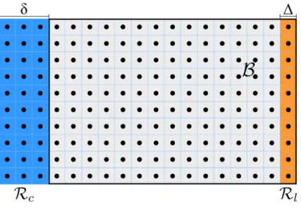
Figure 2.4: Application of boundary conditions in PD.

In the above figure, DBCs including displacements and velocities are applied to all the mate-rial points in Rcwhich will be reflected to the material points within the body B. Regarding tractions and other external forces, they cannot be directly applied to a peridynamic contin-uum but must be expressed as force densities enforced through a material layer _Rl near the domain boundary [14, 3].

2.6

Correction Procedures

2.6.1

Volume correction

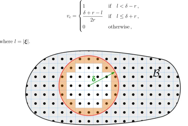
In order to improve the accuracy of the solutions, a volume correction procedure is applied to the material points lying on the horizon [3] by implementing partial volume algorithms. Let ∆ denote the spacing between material points in a uniform grid and r = ∆/2.

As proposed by Hu, Ha and Bobaru [51], an improved algorithm to compute the volume correction factor is as follows

vc=            1 if l < δ_{− r ,} δ + r− l 2r if l ≤ δ + r , 0 otherwise , (2.52) where l =|ξ|.

Figure 2.5: Illustration of full and partial volumes within a neighborhood.

In Fig. (2.5), the material points in white have full volumes whereas the ones in orange have partial volumes since they are located at the limit of the neighborhood.

2.6.2

Surface correction

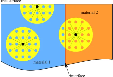
In the BB-PD and OSB-PD formulations, the material models are derived assuming that the material points located in the bulk, i.e., having a full neighborhood. This assumption is no longer valid in the vicinity of free surfaces and/or material interfaces, where material

points have incomplete neighborhoods due to truncated horizons. This phenomenon affects the accuracy of the solution as it alters the material properties in these regions. As a result, corrective procedures are required.

Figure 2.6: Material points’ neighborhoods near free surfaces and interfaces.

Fig. (2.6) depicts the states of neighborhoods within the bulk; near the domain boundary, where the neighborhood is incomplete and across material interfaces, at which a neighborhood consists of material points of different properties. For the BB-PD and OSB-PD formulations, given that the values of the parameters b and d in Eqs. (2.16) and (2.17) are dependent on the integration domain, i.e., the neighborhood, corrective procedures are required. To address these surface effects, various techniques have been developed to compute surface correction factors [52, 3]. According to the technique described in [3], surface correction factors are obtained by computing the ratio of the CCM strain energy density with the PD strain energy density assuming simple loading cases in each spatial direction. Such a procedure is not required in the context of the NOSB-PD formulation. For a correspondence material model, the evaluation of F need not be over a full neighborhood.

Chapter 3

Material and Damage Models

3.1

Constitutive Model

The state-based formulation of PD allows the generalization of the initial bond-based model by accounting for volumetric changes and rotations [15]. It is shown that Eq. (2.31) satisfies

the linear momentum balance for any bounded body B, regardless of the evaluation of T .

Indeed, rearranging Eq. (2.31)and integrating over the body B gives ∫ B (ρ ¨u(x, t)− b(x, t)) dVx = ∫ H{T [x, t]⟨ξ⟩ − T [x ′_{, t]⟨−ξ⟩} dV} x′dVx (3.1)

Given that T [x, t] = 0 when x′ ∈ H/ x, changing the domain of integration fromHx toB and applying change of variables such that x′ = x, Eq. (3.1) becomes

∫ B (ρ ¨u(x, t)− b(x, t)) dVx = ∫ B ∫ B{T [x, t]⟨ξ⟩ − T [x, t]⟨ξ⟩} dVx ′dV_x = 0 (3.2)

According to [15], for any deformation of _{B associated with the constitutive model defined} by T , the angular momentum balance holds

∫

B

The constitutive model is such that ∫

H

Y⟨ξ⟩ × T ⟨ξ⟩ dVξ = 0 ∀Y ∈ V (3.4)

It is noted that T is assumed to be bounded and Riemann-integrable on H.

Indeed, using Eqs. (2.1) through (2.4), (2.30), (2.31), ∫ B y × (ρ ¨u− b) dVx = ∫ B (x + u) × (ρ ¨u− b) dVx = ∫ B ∫ B (x + u) × (T [x, t]⟨ξ⟩ − T [x′, t]⟨−ξ⟩) dV_x′dV_x = ∫ B ∫ B (x + u) × T [x, t]⟨ξ⟩ dVx′dVx − ∫ B ∫ B (x + u) × T [x′, t]⟨−ξ⟩ dVx′dVx = ∫ B ∫ B (x + u) × T [x, t]⟨ξ⟩ dVx′dVx − ∫ B ∫ B (x′+ u′) × T [x, t]⟨ξ⟩ dVxdVx′(variable change) =− ∫ B ∫ B ((x′+ u′)− (x + u)) × T [x, t]⟨ξ⟩ dVx′dVx =− ∫ B ∫ B ((y′ − y) × T [x, t]⟨ξ⟩ dVx′dVx =− ∫ B ∫ H Y⟨ξ⟩ × T ⟨ξ⟩ dVξdVx = 0

For practical applications, it is desired that the peridynamic material response is analogous to that of a CCM material model. The NOSB-PD formulation allows the incorporation of a material model from CCM into the constitutive relation to evaluate the force state. Through the deformation gradient tensor F based on the deformation state Y , the following

correspondence may be established, within the context of homogeneous deformations

Ω(Y ) = W (F (Y )) , (3.5)

where Ω denotes the strain energy density of the peridynamic material model and W that of the CCM material model. Numerous studies dealing with quasistatics in NOSB-PD employ a linear elastic material model.

In this work, it is desired to investigate the behavior of structures undergoing large defor-mations. In order to account for geometric nonlinearity, hyperelastic material models are considered. For such materials, the constitutive relation derives from a strain energy density (SED) function. In particular, the Neo-Hookean material model is employed. The following SED function is considered

W = 1

2λ (ln J )

2₊1

2µ (F : F − 3 − 2 ln J) , (3.6) where J = det(F ) denotes the determinant of F , λ and µ the Lamé parameters.

From Eq. (3.6), the Piola stress tensor is obtained as

P = ∂W

∂F = λ ln J F

-T

+ µ (F − F-T) (3.7)

3.2

Damage Models

Owing to its formulation and meshfree discretization, the peridynamic theory has been successfully used to analyze crack initiation and propagation under various loading condi-tions [22, 18]. A major feature of PD is that damage initiation and propagation are achieved through irreversible bond rupture, the latter is governed by a pre-defined damage criterion. In the case of pre-cracked bodies, the analysis is carried out such that, prior to the integration, all bonds passing through crack surfaces are permanently terminated.

Several criteria are available including the critical stretch, the equivalent and averaged volu-metric strain failure criteria [20], the energy-based criterion [53] and the cumulative damage model for rate-dependent constitutive models [22, 23].

Within the context of quasi-static analysis, the damage criteria are associated with the critical energy release rate Gc, i.e. based on the Griffith theory. The critical stretch schas originally

been derived within the BB-PD theory [39] and is expressed as

sc= √

5 Gc

For state-based material models [3], the critical stretch is sc =                      v u u u t Gc ( 6 πµ + 16 9π2(κ− 2µ) ) δ in 2D , v u u u u t Gc ( 3µ + ( 3 4 )4( κ− 5 3µ )) δ in 3D (3.9)

At every time step, the deformation of a bond is monitored and compared to sc by means of

a history-dependent, scalar-valued function µ such that

µ(ξ, t) =    1 if s < sc ∀t > 0 , 0 otherwise (3.10)

The damage state of a material point is quantified by a quantity referred to as the local

damage index given by

φ(x, t) = 1− ∫ H µ(ξ, t) dV′ ∫ H dV′ , 0⩽ φ(x, t) ⩽ 1 (3.11)

A local damage index of 1 means that all the bonds associated with the material point are broken.

The energy-based damage criterion [53] is such that

µ(ξ, t) =    1 if wξ < wc ∀t > 0 , 0 otherwise , (3.12)

where wξ = (T [x, t]⟨ξ⟩ − T [x′, t]⟨−ξ⟩) · η is the energy density in a bond and wc = 4Gc πδ4 denotes the critical energy density.

Chapter 4

Numerical Implementation

4.1

Discretization of Equations

At a material point xk, the discretized form of Eq. (2.31) is

ρ ¨u(xk, t) = m

∑

j=1

(T [xk, t]⟨xj − xk⟩ − T [xj, t]⟨xk− xj⟩)(vcVj) + b(xk, t) , (4.1)

where m denotes the total number of material points in the neighborhood of xk, Vj the

volume of material point xj and vc is the volume correction factor for the material points

lying on the limit of the neighborhood.

It is worth mentioning that, for each material point, the partial volumes of all its neighbors are computed and stored as an array. These partial volumes will then be retrieved by the appropriate routines for the computations of K, F and the internal force density vector. Furthermore, the shape tensor is approximated as

K =

m

∑

j=1

Using the distributive property of the dyadic product and Eq. (2.30), the approximate de-formation gradient tensor is evaluated as

F = [ _m ∑ j=1 ω(|xj − xk|)((uj− uk)⊗ (xj − xk))(vcVj) ] K−1+ I , (4.3)

where I is the identity matrix.

4.2

Internal Force Density Computation

Within the context of quasi-static analysis with implicit time integration, the routine that evaluates the internal force density (IFD) vector is the principal component of a PD code. For the implicit time integration, a nonlinear solver which uses the Newton-Raphson method calls the IFD routine for the tangent stiffness matrix assembly and the residual vector eval-uation.

The internal force density routine is designed such that:

• The evaluation of T [xk, t] is not repeated when computing the summation in Eq. (4.1).

Hence, a direct approach to evaluating the summation may lead to incorrect entries in the IFD vector.

• The implementation accounts for potentially different material models at each material point in a bond.

The algorithm for the evaluation of the IFD vector is attached in the Appendix.

4.3

Tangent Stiffness Matrix Approximation

The tangent stiffness matrix (TSM) is crucial for the solution of nonlinear systems of equa-tions using Newton-based methods. The entries of the TSM are approximated using the central difference method. The entries of K are defined as

Kij = ∂fint

i ∂uj

where fint

i denotes the i-th component of the global IFD vector and uj the j-th component

of the global displacement vector u.

Based on the approach presented in [54], the following strategies were adopted:

• The entries in K are computed by means of the central difference method. The partial derivative in Eq. (4.4) is approximated as

Kij ≈

f_iint(u + ϵj)− f_iint(u− ϵj)

2ϵ , (4.5)

where ϵ is the unique nonzero entry corresponding to the j-th degree of freedom in ϵj_,

the global perturbation vector.

• The perturbation value must be carefully chosen; it should be sufficiently small relative to the quantities of interest (in this case the displacement values) but not excessively small to avoid subtractive cancellation.

• The perturbed displacement vector is constructed based on the displacements of a material point and its neighbors only.

• A submatrix is used to account for the contribution of each material point into the global stiffness matrix K using a vector of global indices.

Despite the large body of literature on PD, the structural properties of K namely its sparsity pattern as well as its symmetry, are not fully understood. The current work aims to provide a deeper insight into the peridynamic tangent stiffness matrix.

4.4

Time Integration

When inertial effects are negligible, the problem is considered quasi-static. Therefore, Eq. (2.31) becomes

∫

H

{T [x, t]⟨x′_{− x⟩ − T [x}′_{, t]⟨x − x}′_{⟩} dV}

x′ + b(x, t) = 0 (4.6)

In contrast to explicit methods, implicit methods are more stable despite their higher com-putational cost. Given that the governing equation Eq. (4.6) is a nonlinear function of displacement, the implicit integration scheme requires a nonlinear solver.

Eq. (4.6) is linearized as follows

m ∑ j=1 (T [xk, t]⟨xj − xk⟩ − T [xj, t]⟨xk− xj⟩)(vcVj) | {z } fint + b(x_{| {z }}k, t) fext = 0 (4.7) fint(un) + ∂f int ∂u   un | {z } K(un₎ ∆u + fext= 0 (4.8)

Therefore, at every iteration n, the following system of equations is solved

K(un) ∆u =−r , r = fint+ fext, (4.9)

where K denotes the TSM and r the residual vector.

An efficient and correct assembly of the K matrix is thus crucial for the solver to yield correct results.

Prior to the solution, specific operations must be carried out on the system in Eq. (4.9): • When DBCs are enforced, if their values are zero, the contributions of the corresponding

degrees of freedom (DOFs) are omitted, i.e., the appropriate rows and columns in K may be deleted or set to zero.

to the DOFs of nonzero DBC values are modified so as to stabilize the behavior of the system during the iteration process.

The standard Newton-Raphson method is in general locally convergent; its convergence rate is quadratic provided that the initial guess is close enough to the solution and that the Jacobian matrix is not ill-conditioned. However, in practice, these conditions may not be met due to the nature of the problems. As a result, the Newton-Raphson method may exhibit poor performance.

Given the aforementioned issues, the Newton-Raphson method is enhanced with a backtrack-ing line search algorithm so as to achieve global convergence [55]. The next displacement iterate after solving Eq. (4.9) is therefore

un+1 = un+ λ∆u , (4.10)

where λ is the line search parameter that adjusts the Newton step ∆u.

4.5

Solver Design

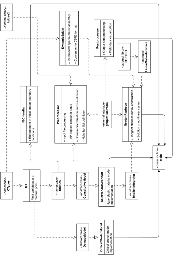
The solver is developed in C++ and exploits the main features of the language including data encapsulation, inheritance, polymorphism as well as dynamic memory allocation. The design is focused on minimal complexity, reduced number of dependencies, maintainability and extensibility. Specific computations and data processing are carried out by means of libraries and utilities. The architecture of the code is depicted in the Appendix.

4.5.1

Neighbor search

The meshfree nature of the discretization requires the construction of a neighbor list for each material point in the domain. Such an operation is crucial since the neighbor list will be used in all subsequent computations. Given the potentially large number of material points, the brute-force approach is inefficient since it has an O(N) time complexity, where N is the size of the data; in this case, the total number of material points.

A more efficient approach is the use of space-partitioning data structures such as k-d trees for which the nearest neighbor search for all the material points takes_{O(logN) on average [56]. In} this project, the neighbor search is carried out with the KDTREE2 library which implements

a k-d tree algorithm on Euclidean spaces.

Tool Functions

Armadillo [57] • Provides MATLAB®_{-like routines}

• Used for constraint region generation

Boost Provides auxiliary containers for data

manage-ment

KDTREE2 [56] • Implements a spatial data structure

• Used for neighbor list construction

PARDISO [58, 59, 60] Used for the solution of linear systems

gnuplot-iostream Used for data visualization

Table 4.1: Dependencies of the solver

4.5.2

Representations of sparse matrices

Sparse matrices are often encountered in scientific and engineering problems during the nu-merical solution of differential equations. Given their structures - the number of nonzero elements is significantly smaller than the matrix size - it is essential to use appropriate data structures to store only the nonzero entries as well as particular algorithms to manipulate them.

4.5.2.1 Storage schemes

Various storage schemes are available for sparse matrices including the Compressed Sparse Row (CSR), Compressed Sparse Column, Coordinate and Block Compressed Sparse Row formats. These storage schemes are static data structures since they are defined in terms of fixed-size arrays.

In contrast, dynamic data structures are more flexible due to run-time memory allocation. Vectors of the C++ Standard Template Library, linked lists and binary search trees are among the most common dynamic data structures.

the incremental matrix assembly with a dynamic data structure followed by the conversion of the latter into the more compact CSR format.

4.5.2.2 Incremental matrix assembly

The approach adopted herein is similar to that proposed by Jansson [61] who proposed a stack-based representation for sparse matrix assembly. In this project, the tangent stiffness matrix is populated by means of a hash table. To reduce the complexity of the implementa-tion, the hash table is implemented as an array of singly linked lists. The data structure has been designed such that only the nonzero elements are stored.

The output of the assembly, after the necessary modifications, is the global stiffness matrix stored in the CSR3 format.

The latter consists of three arrays:

• Let n denote the number of rows of the square matrix and nnz the number of nonzero entries. a is an array of length nnz that stores the nonzero entries.

• ja is an array of length nnz which stores the column indices of the nonzero entries in the original matrix.

• ia is an array of length n + 1 which stores the indices in a corresponding to the first nonzero entries in each row. It is noted that the last element in ia must be nnz and that the number of nonzero entries per row is ia[i + 1]− ia[i], i = 0, · · · , n, following a zero-based indexing.

For example, given a sparse matrix A

A =       1 −1 0 −3 −2 5 0 0 0 0 4 6 −4 0 0 7      

Using the zero-based indexing, the CSR3 representation of A is thus a = ( 1 −1 −3 −2 5 4 6 −4 7 ) , ja = ( 0 1 3 0 1 2 3 0 3 ) , ia = ( 0 3 5 7 9 )

Chapter 5

Discussion and Conclusion

5.1

Discussion

Various features of the peridynamic theory have been considered within the scope of the current work. Notably, the enforcement of BCs is one of the most challenging aspects of the problem considering the nature of the formulation; constraints are applied through material layers. Since the minimum thickness of the constraint region (Fig. (2.4)) is the horizon size, there is no restriction on the number of material points within the constraint regions. Therefore, the total number of DOFs in the system depends on the implementation. For the aforementioned reasons, the performance of a PD solver may be improved by exploiting the symmetry of the geometry whenever applicable [62].

Since PD simulations are computationally expensive, it is necessary to implement techniques that reduce storage requirements and computation time. For instance, a knowledge of the features of the TSM can be exploited to boost the efficiency of the solver; if the TSM possesses

numerical symmetry, only its upper or lower triangular part needs to be stored and passed

to the linear solver. The TSM assembly is a major bottleneck during the simulation given the method used to compute its entries along with the required modifications prior to the solution of the linear system of equations. Therefore, cache-friendly data structures should be used to store the sparse matrix; for example, containers with contiguous memory storage. Furthermore, parallelization is required for all practical applications to render the simulations less expensive. Moreover, preallocation of the TSM may be advantageous.

It is also noted that more advanced algorithms may be used for the volume correction proce-dure, at the expense of increased complexity [63]. It has been demonstrated that the volume correction procedure greatly affects the convergence of the solution [64, 63].

On the physical significance of the horizon, it is worth mentioning that, at the macroscale, a material modeled with the peridynamic formulation is assumed to possess an underlying microstructure [65] since the interactions between the material points within a body need not be physically meaningful; the horizon is a mathematical quantity that appears in the governing equation and may be calibrated with other parameters including grid spacing to reproduce the material properties. However, the horizon δ must reflect the appropriate length scale dictated by the physics of the problem; nonlocal effects are prominent for problems including nanoscale structures and fracture [66].

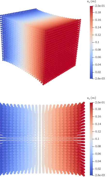
Figure 5.1 illustrates the deformation of a unit cube calculated by the peridynamic code developed here subjected to a displacement loading of magnitude d = 0.2 along its front face and fixed along its back face. The material parameters are E = 2.5 and ν = 0.45. The cube is discretized into 25 material points along each edge and the horizon size is chosen such that