I . I N T R O D U C T I O N
The idea that the real rate of interest is not fixed is not new and is addressed in Choudry, et al. (1991). Fisher (1979) and Rose (1988) also investigated the presumed stationarity of the real rate of interest.
In this short paper, we would like to approach the issue of stationarity of the real rate from a different angle emphasizing an information processing behaviour. Our starting point will be the choice-theoretic structure and the analysis of real interest behaviour within that context. The issue is best elaborated in Hirschleifer (1970). The optimization of utility over different consumption claims is satisfied by
(1) where r1is the real rate of interest. If uncertainty is allowed in this two period model, market agents are also required to consider the possible states of the world upon which the receipt of future consumption claims depend. Let us define c1A and c1B as alternative consumption claims for future period 1 with respective
(subjective) probabilities of occurrence p 1
A and p 1Bin two alternative states A and B. Maximization of expected utility in such a setting, as shown by Hirschleifer, requires the following equilibrium conditions
(2)
(3) where r1Aand r
1Bare risky real rates for the alternatives A and B.1
The results can be generalized to N individuals by utilizing weighted averages for the utility function and the probability assignments leading to market rates. Equations 2 and 3 imply that
- 1 1 + r1B = p A¶ u (c0, c1A) ¶ c0 +p B ¶ u (c0, c1B) ¶ c0 p B¶ u (c0 , c1B) ¶ c1B - 1 1 + r1A = p A ¶ u (c0, c1A) ¶ c0 +p B¶ u (c0, c1B) ¶ c0 p A¶ u (c0 , c1B) ¶ c1A - 1 1 + r1 = ¶ U / ¶ c0 ¶ U / ¶ c1
A choice-theoretic and information-oriented
approach to the short-run characteristics of
real and nominal interest rates
U MI T E RO L a n d E RO L M . BA L K A N
Department of Economics, Bilkent University, Ankara, Turkey and Department of Economics, Hamilton College, Clinton, NY 13323, USA
Received 8 February 1995
The paper adopts a choice-theoretic, information-oriented approach to the issue of stationarity of real interest rates. It is shown that a constant real rate of interest, even for short run and within the context of a simple two-market framework, requires overly demanding assumptions which are unlikely to be satisfied if efficient market hypothesis is explicitly considered. Such a model which indirectly supports the short-run variability of real interest rates in response to random information signals is tested empirically by utilizing multiple time series models for the 1959–87 observation period. The empirical results suggest a favourable interpretation of the model.
1350–5851 © 1995 Chapman & Hall 191
1The existence of two risky real interest rates for the same period corresponds, in the actual world, to variation in interest rates on assets of
real interest rates are functions of the probabilities assigned to future events and the market participants’ utility functions in a world of uncertainty. In what follows, we will attempt to describe a framework which shows and tests how this insight may lead to short- run non- stationarity of the real rate of interest.
The first step is to explicitly associate the sets of equations above with the concept of information and efficient market hypothesis. We can write p A(A), p B(A), . . . , p N(A), where A is a general set of information that is utilized by a representative market agent in the current period to assess the possible states of the world.2 This form implies that the probabilities assigned to future events are based on all currently available information under the efficient market hypothesis. The incorporation of a new signal can affect the subjective probabilities of a representative agent (and the average probabilities of aggregated market participants) and hence, through Equations 2 and 3, the real interest rate. Then it is clear that the real interest rate may be subject to change, even over a short time period.
A second step that logically follows from a careful interpretation of the equation set is the following one. A change in the probabilities change the real price of future consumption claims in terms of present consumption claims. If the analysis is confined to a two-market (bond/commodity) framework for the sake of simplcity, two results follow from the earlier premises mentioned. The first relates to the fact that the same information bit liwould lead to adjustments in both commodity and bond markets.
This follows from the fact that new information lithat increases (decreases) the premium on present consumption versus future consumption would theoretically increase (decrease) the demand for present consumption. Given that market participants are utility maximizers, this would simultaneously lead to higher (lower) demand for commodities, a negative (positive) effect on the real demand for bonds and a positive (negative) effect on the real supply of bonds. The latter two effects follow from the fact that bonds entitle their holders to higher future consumption claims in return for lower present consumption possibilities. It is evident that the real interest rate will change simultaneously with the commodity demand in response to the same information bit. The foregoing analysis indicates the theoretical possibility of certain states of the world where a new information bit (signal) l iwould lead to short-run adjustments in both the real interest rate and prices. To the degree that new information l iaffects the present consumption claims for most of the traded goods, the information originated short-run variations will be observed in both the real interest rates and the change in the general price level (actual inflation rate) in a contemporaneous way. The next section develops a testable framework for the arguments utilizing a multiple time series approach and presents empirical results. The last section summarizes the conclusions.
I I . A T E S T A B L E F R A M E W O R K B A S E D O N M U L T I P L E T I M E S E R I E S MO D E L S
The following equation is proposed as a starting point for the several arguments that will follow:
R·= r·+ E· (4)
where R·is the first difference of log R, r· is the first difference of log r and E·is the first difference of log E. The variables R, r and E respectively denote the nominal interest rate, the real interest rate and inflationary expectations. Equation 4 posits a relationship which is similar in content but different in form with respect to the Fisher hypothesis. The purpose of proposing the form in Equation 4 is twofold. First, it transforms all variables into a nearly stationary form which will be of practical convenience for us in the rest of the analysis. Second, it expresses the relationship between the nominal interest rate, real rate and expected inflation in terms of rates of change rather than levels. Hence it allows us to interpret the effect of new information as signaling expected deviations from historical trends. This view assumes that trends of actual variables are determined by the long-run tendencies of economy-wide factors and systematic influences. The novel information in our context is of random nature and is assumed to affect the real rate expectations by changing the probability assignments. Hence we are referring to a set of mostly weak signals which are potent enough to change the subjective state probabilities but not potent enough to cause a trend reversal by themselves. Thus we assume that the type of information which may affect the state probabilities is generated and incorporated into the information set in a random manner.3
The right hand side of Equation 3 can be written as
R·= r·[ l-r] + E·[ l-E] (5)
where r·= r·[l-rand E·= E·[l-E].
The first term specifies that the rate of change of the expected real rate is generated by information vector l-rwhere all elements l i
rof vector l
-rsatisfy the condition of affecting the state
probabilities and consequently the expected real rate. The second term specifies that the rate of change of expected inflation is generated by information vector l-Ewhere all elements l i
E of
vector l-E satisfy the condition of affecting expectations of inflation.
Assuming that the elements l i
r and l iE are generated
randomly, Equation 4 can be written as:
R·= A (L)e r+ B (L)e E (6)
2A is any kind of publicly available information actively utilized in the assessment of future states of the world, e.g., policy decisions, money
announcements, international events, etc.
3This view may be partially supported by the fact that the time series of US nominal interest rates apart from a seasonal autoregressive
component may be modelled as a MA1 or MA2 process. The real interest rate and expected inflation components are non-observable and any tests associated with them can only be undertaken through a more indirect approach by using multiple time series.
We also introduce an inflation vector in the form of
X· = C(L)e r + D(L)e E (7)
which describes the rate of change of the actual inflation rate as a moving average representation of its own distributed innovations and the innovations of the real interest rate. The logic of introducing Equation 6 follows from earlier discussions. A direct test of the short-run variability of the real rate of interest avoiding proxies is very difficult given its ex ante nature. An indirect test, however, may be possible. Following the rigorous interpretation of the choice-theoretic approach and the arguments set forth in the first section, we require the trend- free components of inflation vector and particularly the real rate vector to be responsive only to short-term, non-persistent innovation terms. Moreover, these innovation terms should be contemporaneously correlated in order to be compatible with the common response behaviour of real rates and price movements to the same set of signals. Then we combine Equations 5 and 6 as:
R·= A (L)e r + B (L)e E (8)
X· = C(L)e r + D(L)e E (9)
Though it is difficult to distinguishe rand e Eon an observational level, Equations 7 and 8 imply multiple feedback effects between the X·and R· vectors. This suggests a multiple time series model which can be empirically tested in the form:
R·= q 11a1 (t–1) + q 12a1 (t–2) + · · · + q 1na1(t–n)
q 21a2 (t–1) + q 22a2 (t–2) + · · · + q 2 (t–n)a2 (t–n) (10) X· = q 11a1(t–1) + q 12a1 (t–2) + · · · + q 1na1 (t–n)
q 21a2 (t–1) + q 22a2 (t–2) + · · · + q 2 (t–n)a2 (t–n) (11) This defines an nth order moving average process for two variables in a multiple time series setting. Note that R· is the first difference of the logarithm of nominal interest rates, while X· is the second difference of the logarithm of the actual inflation rate.4
We expect upon estimating the model that: a) the component of real rate and inflation series which do not include unit roots can be jointly modelled as a low-order moving average process rather than an autoregressive process showing that this component is dominated by random responses to information signals,
b) the cross-correlation matrix between R· and X· is non-triangular showing the contemporaneous or nearly contemporaneous correlation between the innovation terms.
I I I . E MP I R I C A L RE S U L T S
We estimated a multivariate model with the nominal interest rate and inflation rate as variables for the 1959–87 period. A total of 340 monthly observations are used.5 The data for interest rates are 90 day monthly treasury bill yields from the Federal Reserve Bulletin. This choice is motivated by the expected higher sensitivity of T-bill yields to new information in the short-run given the depth of the secondary market. The sensitivity of T-bill yield to the inflation-related information content embedded in money announcement information is cited elsewhere (Cornell, 1983). The inflation rate series is constructed by taking the first difference of the natural logarithm of the consumer price index (CPI). The stationarity inducing operations are applied to the series. The outline described by Tiao and Box (1981) and Jenkins and Alavi (1981) is utilized for the identification, estimation and diagnostic checking stages of the model.
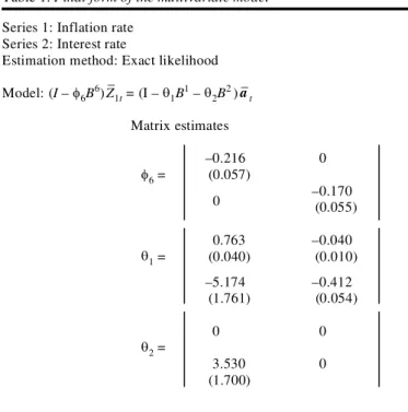
The identification and estimation stages suggested the following model:
(I – f 6B6)Z–
l t= (I – q 1B1– q 2B2)a–t (12)
as the most parsimonious model on the basis of diagnostic checking. The 2 ´ 1 vector Z contains the transformed inflation and nominal interest rate series, and a is a 2 ´ 1 vector of independently distributed random shocks. The parameters are contained in the 2 ´ 2 matrices f 1, q 1and q 2. The parameters were first estimated by conditional least squares and then re-estimated by the exact likelihood method.6 The determinants of the estimated q and f matrices have their roots outside the unit circle, satisfying the invertibility and stationarity conditions. Table 1 gives the sample estimates of the matrices. The residual diagnostic checking (Table 2) confirms that the model transforms all the sample cross- correlation matrices approximately into realizations of white noise process. Splitting the data into two or three parts and re-estimating the model did not change the content of the results. The generating mechanism for the data is more easily seen using the following explicit form:
(1+ 0.21B6)X
t= (1 – 0.73B)a1 t+ 0.04a2 t (13) (1+ 0.17B6)R
t= (5.17 – 3.53B2)a1 t+ (1 + 0.41B)a2 t (14) 4The first difference of the logarithm of the actual inflation rate display a strong systematic term particularly in the second moment. Hence we
required a second differencing. Studies of monthly US inflation rate suggest a second unit root as illustrated by Schwert (1987) which seems to be eliminated by the second differencing.
5The observation period, more exactly, is from January 1959 to December 1987. Earlier periods were not considered because of interest rate
pegging prior to 1951 and its possible effects in the subsequent years. Though higher data frequency is desirable in a study which is information oriented, the obvious restraint is the availability of only monthly data for the actual inflation rate.
6Conditional least squares may give unstable and biased estimates of the parameters in the moving average operator. The exact likelihood
method proposed by Ansley (1979) and Hillmer and Tiao (1979) is an alternative algorithm to derive more efficient moving average parameter estimates.
In Equations 13 and 14, Rtis the first difference of the logarithm of nominal interest rates, Xtis the first difference of the logarithm of the actual inflation rate, a1 tis the innovation driving the
inflation rate and a2 tis the innovation driving the nominal interest rates and B is the lag operator satisfying BX = Xt–1, B2X = X
t–2, etc.
The model is dominated by moving average terms. The inflation rate series is driven by the innovations of the interest rate with a short lag and the interest rate is driven by lagged innovations of the inflation rate. The existence of sixth-order autoregressive parameters may imply residual seasonal correlation.7
The empirical results seem to be supportive. There is a direct empirical support to the fact that the components of nominal interest rates and inflation rate that are free of unit roots are dominated by low order innovation terms and results indicate contemporaneous correlation between these innovation terms as would be suggested by the framework outlined in section I.8
I V . CO N CL U S I O N
In this paper, we adopted a beginning point borrowed from the choice- theoretic structure of the interest rates. When such a model is associated with the efficiency hypothesis and an information-oriented interpretation, it may imply the short-run variability of the real interest rates. This however, is not directly testable. Hence we reverted to the empirical testing of the other observable features of the model which follow from the model itself. An empirical test employing multiple time series methodology and applied to US data seem to support the predictions of the model. Hence the results may be interpreted as indirectly supporting the short-run variation of the real interest rates. At least, the necessary conditions, if possible not the sufficient conditions, seem to be satisfied for the model. The more direct results of the study are
Table 1. Final form of the multivariate model Series 1: Inflation rate
Series 2: Interest rate
Estimation method: Exact likelihood Model: (I – f 6B6)Z– 1t= (I – q 1B1– q 2B2) –at Matrix estimates –0.216 0 f 6= (0.057) –0.170 0 (0.055) 0.763 –0.040 q 1= (0.040) (0.010) –5.174 –0.412 (1.761) (0.054) 0 0 q 2= 3.530 0 (1.700)
Note: Only the statistically significant estimates are reported as coefficients. The statistically insignificant coefficients at the 95% level are reported as 0. Standard deviation estimates are in parentheses.
Table 2. Residual diagnostic checking Lags 1 through 6 · · · · · · · + · · · · · Lags 7 through 12 · · · · · – · · · · Lags 12 through 18 · · · + · · · · Lags 19 through 24 – · · · · · · · – · · · · Lags 25 through 30 – – · · · · · · · · Lags 31 through 36 · · · – · · · ·
7In a frequency domain sense, the frequency corresponding to a sixth month cycle is the first harmonic of the frequency corresponding to a
seasonal twelve month cycle. The following harmonics are at frequencies corresponding to 12/3, 12/4, 12/5 . . . months. Strong aliasing effects may cause a broad, strong peak nearly corresponding to a sixth month cycle which may not be adequately attuned by a logarithmic transformation.
8Admittedly the two-market model employed here is too restrictive. However, it enables direct comparison with Fisher hypothesis which depends
on similar restrictions. Also the model becomes very complex deterring anything meaningful even at a three-market level. For example, we estimated a three-vector model including money supply proxied by M1A. Money variable required a set of complicated transformations such as logarithmic transformation, first differencing and seasonal differencing to be transformed into stationary form. All three series turn out to be correlated by own and cross innovation terms, but the lag structure is complex because of the multiplicative seasonal polynomial. The innovation lag structure was simplified by eliminating those parameters that are not significantly different zero but still the remaining structure was complex.
the domination of stationary vectors of nominal interest rates and inflation rate by random factors and the nearly contemporaneous correlation between the innovation terms of the inflation and nominal interest rate vector. This last point may indicate a common response of prices and interest rates to information signals in the short run.
RE F E R E N CE S
Ansley, C. F. (1979) An algorithm for the exact likelihood of a mixed autoregressive-moving average process, Biometrika, 66, 59–66. Choudry, T., Placone, D. and Wallace, M. (1991) Changes in the fisher
effect in the 1980s: evidence from various models, Journal of
Economics and Business, 43 (1), 59–68.
Cornell, B. (1983) The money supply announcement puzzle: review and interpretation, American Economic Review, 73, (4) 644–57.
Fisher, S. (1979) Anticipation and the nonneutrality of money, Journal
of Political Economy, 87, (2) 225–52.
Hillmer, S. C. and Tiao, C. C. (1979) Likelihood function of stationary multiple autoregressive moving average models, Journal of the
American Statistical Association, 74, 632–60.
Hirschleifer, J. (1970) Investment, interest, and capital, Prentice-Hall, Inc. New Jersey.
Jenkins, G. M. and Alavi, A. S. (1981) Some aspects of modeling and forecasting multivariate time series, Journal of Time Series Analysis, 2, 1–47.
Rose, A. K. (1988) Is the real interest rate stable?, Journal of Finance 43 (5), 1095–112.
Schwert, G. W. (1987) Effects of model specification on tests for unit roots in macroeconomic data, Journal of Monetary Economics, 20 (1), 73–103.
Tiao, G. C. and Box, G. E. P. (1981) Modeling multiple time series with applications, Journal of the American Statistical Association, 76, 802–16.