RESEARCH PAPER
An Empirical Assessment of the Contagion Determinants
in the Euro Area in a Period of Sovereign Debt Risk
Hazar Altınbaş1 · Vincenzo Pacelli2 · Edgardo Sica3
Received: 4 September 2020 / Accepted: 25 February 2021 © The Author(s) 2021
Abstract
This paper uses learning methods and optimization techniques to investigate the determinants of shock propagation in the Euro area for the period 2001–2015. First, principal component analyses are used with country bond yields to identify sub-periods and country groups; second, influencing factors for country bond yields are investigated with random forest models; lastly, shock propagation among groups are examined with impulse response functions. Models in steps two and three are improved by using simulated annealing algorithm. The empirical findings achieved can be particularly relevant for both investors and policymakers. Shedding light on the determinants of financial contagion may be in fact useful for investors who can derive relevant information about countries which are less sensitive to be affected by shocks, orienting thus their investment strategies. At the same time, policymakers could draw worthwhile and preventive hedging strategies and design the most suit-able crisis management policies.
Keywords Contagion · Euro area · Sovereign debt · Time-series analysis · Machine learning · Optimization
JEL Classification C3 · C4, · 61 · F36 · G1
* Edgardo Sica [email protected]
1 Department of Banking and Finance, Beykent University, Istanbul, Turkey
2 Ionic Department in Legal and Economic System of Mediterranean: Society, Environment,
Culture, University of Bari Aldo Moro, Bari, Italy
3 Department of Economics, Management and Territory, University of Foggia, via A. da Zara 11,
1 Introduction
In the last 20 years, economic literature has devoted a large amount of effort into investigating contagion, i.e. the unexpected transmission of shocks across coun-tries (Rigobon 2016). Although some evidence of contagion can be traced back to the Great Depression in 1930s and to the Debt Crisis in 1980s, the first empirical contributions were only produced in the 1990s, and specifically after the Mexican (1994), Asian (1997), and Russian (1998) currency collapses. The intensity of the propagation mechanisms that characterized these shocks greatly surprised both academicians and practitioners. Indeed, whereas it is reasonable to expect that large countries suffering crises may influence smaller countries (as happened dur-ing the Great Depression), or that shocks in one country may affect its main trad-ing partner (as in the case of the collapse in Russia in the 1980s that caused the collapse of Finland), in the aforementioned 1990s crises countries were heavily affected by shocks generated in other countries, despite the limited trading links with those countries. In contrast, in those years, other crises produced a confined contagion (or did not produce any contagion at all) as in the case of the Brazilian (1999), Turkish (2000), and Argentinean (2002) crises. This significantly contrib-uted to the increase of interest in studying the drivers of shocks and, above all, the prevention of the related propagation mechanisms (Kaminsky et al. 2003). The 2008 US sub-prime crisis and the 2010 EU fiscal crisis have renewed the interest about contagion, creating a “near-ideal laboratory” for researchers in order to study causes and effects of financial contagion that arise at the time of stress (Longstaff 2010). As happened in the 1990s crises, in both the 2008 and 2010 crises a shock in small and isolated markets produced a huge impact at the global level. Indeed, even though the size of the sub-prime market in 2007 rep-resented a very limited portion of the financial system, it had a massive impact in the US and across the world. Similarly, although Greece contributes in a very limited way to the financial flows in the Euro area, this makes it particularly hard to explain why other countries were affected by the collapse of Greece. Whereas in their recent study, Caporin et al. (2018) show there is no evidence for shift-contagion in European debt crisis, subject is still open to debate.
From an empirical point of view, the proper analysis of the possible conta-gion’s determinants (if any exists) requires the inclusion of many variables into the estimated models. However, due to the increasing number of variables, the dimension of data space increases and observations become sparse and the situa-tion worsens in presence of small samples. In convensitua-tional statistical techniques (in several forms of regression settings), obtaining statistically significance results becomes therefore nearly impossible. Even when significant results are achieved, model assumptions and validity are not hold. In order to deal with high dimensionality, a number of approaches can be employed. One of the simplest examples is to conduct a stepwise variable selection procedure to find the best fitting combination of variables (Siebenbrunner et al. 2017). But as the number of candidate variables increases, this approach quickly becomes time-consuming and mostly not efficient at finding the best or near-best combination of variables.
Today, there are more options to deal with so-called curse of dimensionality, particularly machine learning methods (Athey 2018; Athey and Imbens 2019), combinatorial optimization techniques (Gilli and Winker 2008) and their hybrid forms. Their use in economic empirical research is fast growing providing a valu-able option instead of simplification and misspecification in highly complex prob-lems in economics.
In this framework, the present article contributes to the empirical literature on contagion by investigating the determinants of shocks propagation in the Euro area using data from 2001 to 2015 applying a hybridized approach based on a machine learning, metaheuristic optimization and conventional econometric methods. More specifically, we adopted a three-step methodology. Firstly, we used a principal com-ponent analysis (PCA) on the first differences of countries’ bond yields to reveal any co-movement in bond yields’ changes. This allowed us to divide analysis period into sub-periods and to group countries in sub-groups. Secondly, we employed a ran-dom forest (RF) model with the aim of searching for government bond yields’ deter-minants in the identified sub-periods. Thirdly, impulse response functions (IRF) were produced from estimated vector auto regression (VAR) models. In equations, we used bond yield spreads between groups and focused on those in which spreads were regressed on their own lags along with selected variables’ (from second step) lags. In second and third steps, a simulated annealing (SA) algorithm was used for the variable selection (i.e. for optimization) to increase efficiency and reliability of our results. The improved success of RF learning and diagnosis test results on VAR models confirmed the SA contribution to our objective. We believe therefore that the methodology employed and the robust results achieved in this study contribute to literature in both respects.
Next section reports the literature review followed by the material and methods section. Results are then presented along with discussions, and the paper ends with some concluding remarks.
2 Literature Review
2.1 Definition, Identification, and Explanation of Contagion
Despite the large amount of both theoretical and empirical literature investigat-ing contagion, literature lacks a universally recognised definition of contagion. In their seminal article, Forbes and Rigobon (2002) define contagion as a significant increase in cross-market linkages after a shock to one market. Alternatively, con-tagion can be defined as the propagation of shocks between two markets in excess of what should be reasonably expected (Billio and Pelizzon 2003). Relatedly, Broto and Perez-Quiros (2015) defined contagion as a significant variation in the cross-country co-movements (of CDS spreads) compared with that of non-crisis periods. This definition is consistent with the fact that realization of a reasonable expectation can mostly be possible in calm periods.
In more general terms, contagion can be identified with the process of shock transmission occurring within a complex system (i.e. a system composed of many
elements interacting with each other by means of non-linear dynamics) in both calm and crisis periods (Kaminsky et al. 2003). In this study, we refer to this definition to test the contagion determinants in Euro area. Following such approach, financial system provides a relevant example of a “complex system” where contagion can be conceived as the probability that the instability of a given financial institution (mar-ket, infrastructure, etc.) spreads to other parts of the system, thus creating a negative effect that leads to a wide financial crisis (Allen et al. 2009; Gai et al. 2011; Helbing
2012) and in some cases segmentation in global system.
It is worth noting that banking system is inherently more vulnerable to conta-gion. According to Kaufman (1992), bank failure contagion occurs faster, spreads more broadly within the industry, results in a larger number of failures, causes greater losses to creditors (depositors) at failed banks, and spreads further beyond banking industry. This causes substantial damage to both financial system and macroeconomy.
In order to identify contagion, the literature proposes several different criteria (Smaga 2014). In particular, contagion happens when: (i) the transmission is in excess of what can be explained by economic fundamentals; (ii) the transmission is different from regular adjustments observed in calm times; (iii) the events constitut-ing contagion are negative extremes; (iv) the transmission is sequential, for example, in a causal sense.
Moreover, contagion can happen by means of both direct and indirect channels (Upper 2011). Direct channels are exposures arising from interbank loans, payment systems, and derivative securities. For instance, the fear that a bank might become insolvent stokes a panic that pushes depositors to withdraw their deposits on mass, thus increasing the risk of insolvency of the bank itself. Cases of bank runs hap-pened recently in London due to Brexit, and in Greece and Cyprus in 2015. In addi-tion, interbank connections can act as a contagion channel that exposes banking system to a lack of coordination phenomena (gridlock equilibrium) even when all banks are solvent. Indirect channels include the effects of deterioration in the assets of balance sheet price.
The literature explains contagion by means of three main approaches, namely the fundamental, financial, and coordination views (Rigobon 2016). The funda-mental view concentrates on real channels (such as bilateral trade and macroeco-nomic policies) to explain the propagation of shocks across countries (Corsetti et al. 2000, 2005; Gerlach and Smets 1995). This approach was used mainly to explain contagion deriving from Great Depression, as well as for the 1970s and 1980s crises in Europe. The financial view believes that contagion is caused by constraints and inefficiencies in banking sectors and international equity markets (Goldstein et al. 2000; Kaminsky and Reinhart 2003). The main idea behind this approach is that imperfections in the financial system can be exacerbated dur-ing a crisis, increasdur-ing the propagation of shocks across countries. Finally, the coordination view explains contagion by means of coordination failures among investors and/or policymakers (Calvo and Mendoza 2000; Drazen 2000; Masson
1998). According to this approach, the transmission of shocks occurs because of informational problems that may push market participants to withdraw resources jointly across countries, or policymakers to give up a macroeconomic policy.
More recently some authors (Acemoglu et al. 2015; Gai and Kapadia 2010) have examined how shocks propagate through a network based on debt holdings or interbank lending; also, how shocks propagate as a function of network archi-tecture. Results suggest that incomplete networks are more inclined to contagion than complete ones, and that the more the network is connected, the more it is resistant. This is because the proportion of losses in the portfolio of a bank is transferred to more banks through interbank agreements.
2.2 Contagion Determinants
The literature has proposed several different variables as possible determinants of contagion. In particular, fundamental macroeconomic variables (especially GDP growth rate, GDP per capita, unemployment rate, inflation rate, government debt amounts and GDP ratios) are the more frequently used ones in the empirical stud-ies (Bernal et al. 2016; Boumparis et al. 2015; Bratis et al. 2015; Brutti and Sauré
2015; Dufrénot et al. 2016; Gómez-Puig and Sosvilla-Rivero 2016; Ho 2016). Together with variables that measure financial linkages and regional/global shocks (Gómez-Puig and Sosvilla-Rivero 2016), it is possible to distinguish the effects of the economic situation and interconnections of countries on contagion; this is also known as “fundamentals-based contagion” (Calvo and Reinhart 1996; Kaminsky and Reinhart 2000).
Moreover, some studies suggest that contagion also occurs due to the behav-ioural reactions of investors or market participants, not just because of economic fundamentals (Masson 1999; Mondria and Quintana-Domeque 2013). Benchmark stock market indices, economic policy uncertainty indices, rating announcements from rating agencies, political announcements, economic indicators/information announcements and events are incorporated into models for better understanding the transmission of shocks (Apergis 2015; Baum et al. 2016; Bernal et al. 2016; Brutti and Sauré 2015; Dufrénot et al. 2016; Gómez-Puig and Sosvilla-Rivero 2016; Pra-gidis et al. 2015). These studies generally conclude that contagion transmission is seen as stemming from both fundamentals and market sentiment variables.
Starting from this framework, the present study follows Gómez-Puig and Sos-villa-Rivero (2016) by setting two main variable categories:
1. Market sentiment variables that proxy the participant behaviour in the economy related to existing information. These variables ultimately shape future expecta-tions.
2. Macroeconomic fundamentals variables that proxy the financial and economical linkages that may adversely affect several countries simultaneously.
Within the above two categories, we have defined two sub-categories of vari-ables, namely country-specific and global. In this way, we aim to assess whether cross-country contagion is effective on economic variations, and investigate which indicators primarily influence cash flows and credit collections.
3 Materials and Methods
3.1 Data
In order to assess the determinants of contagion in Euro area, we selected 10 out of 17 countries belonging to Economic and Monetary Union (EMU). These were Aus-tria, Belgium, France, Germany, Greece, Ireland, Italy, Netherlands, Portugal, and Spain. Five of these (Portugal, Ireland, Italy, Greece, Spain; also known as “PIIGS”) are EMU peripheral countries and exhibit serious sovereign debt problems. In con-trast, remaining countries (Netherlands, Austria, Belgium, France, and Germany) are EMU core economies: they are financially stabilised and considered to be “safe-heavens” by investors.
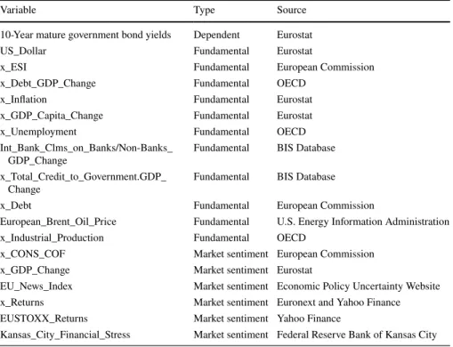
Our initial dataset included 28 global variables. We first reduced the dataset dimension by dropping variables with a correlation score higher than 0.9. Then, we combined the remaining variables (total of 17) with each country-specific variable dataset. A summary of the ultimate variables used in our empirical investigation is reported in Table 11 and description of variables can be found in Appendix A.
Table 1 Types and data sources of variables
Variable Type Source
10-Year mature government bond yields Dependent Eurostat
US_Dollar Fundamental Eurostat
x_ESI Fundamental European Commission
x_Debt_GDP_Change Fundamental OECD
x_Inflation Fundamental Eurostat
x_GDP_Capita_Change Fundamental Eurostat
x_Unemployment Fundamental OECD
Int_Bank_Clms_on_Banks/Non-Banks_
GDP_Change Fundamental BIS Database
x_Total_Credit_to_Government.GDP_
Change Fundamental BIS Database
x_Debt Fundamental European Commission
European_Brent_Oil_Price Fundamental U.S. Energy Information Administration
x_Industrial_Production Fundamental OECD
x_CONS_COF Market sentiment European Commission
x_GDP_Change Market sentiment Eurostat
EU_News_Index Market sentiment Economic Policy Uncertainty Website
x_Returns Market sentiment Euronext and Yahoo Finance
EUSTOXX_Returns Market sentiment Yahoo Finance
Kansas_City_Financial_Stress Market sentiment Federal Reserve Bank of Kansas City
1 x is used as a generic name. Possible abbreviations are: IR (Ireland), DE (Germany), GR (Greece), IT
(Italy), FR (France), PT (Portugal), AT (Austria), NL (Netherlands), ES (Spain), EU (European Union), EA (Euro Area), OECD (Organisation for Economic Co-operation and Development), G7 (United States, Canada, France, Germany, Italy, Japan, United Kingdom), US (United States).
First, we used yields of Euro area sovereign 10-year mature bonds as the depend-ent variable, for PCA and RF. The literature (see, for instance, Cronin et al. 2016; Gómez-Puig and Sosvilla-Rivero 2016; Koop and Korobilis 2016; Singh et al. 2016) uses country bond yield spreads (mostly difference with Germany bond yields) instead of yields, but we initially opted for yields because we did not differentiate Euro area countries as a priori “core” and “peripheral”. After country groups and bond yields’ determinants are identified, mean bond yields of groups are calculated and spreads between groups are used in VAR models. We employed monthly sam-pled observations from 2001:01 to 2015:12; a total of 179 observations for each var-iable for each country.2
3.2 Methodology
As shortly described in introduction, in this study we followed a three-step methodology.
In step 1, PCA on the first differences of countries’ bond yields was used to reveal any co-movement in bond yields’ changes. By exploiting information provided by PCA, we could thus identify disturbances/breaks in co-movements and find evidence on the dissociation of Euro area economies. Analysis period was then divided into sub-periods and countries grouped according to the findings achieved. Within each group, a bond yield variable was calculated by averaging countries’ bond yields. In step 2, an RF model was employed with the aim of searching for the govern-ment bond yields’ determinants in the identified sub-periods. We preferred to use a machine learning method rather than conventional statistical approach (e.g. linear regressions) since RFs are usually more reliable and efficient to determine which variables are more important in predicting yields, especially when relationships are not linear but in complex forms and with a large number of features that are not related to the outcome (Athey and Imbens 2019; Wager and Athey 2018). In step 3, IRF were produced from estimated vector auto regression (VAR) models. In equa-tions, we used bond yield spreads between groups and focused on those in which spreads were regressed on their own lags along with selected variables’ (from step 2) lags. In steps 2 and 3, an SA algorithm was used for selecting variables (i.e. for opti-mization) in order to remove redundant predictors, decrease noise, increase degrees of freedom, and thus enhance efficiency and reliability of our results. Improved suc-cess of RF learning and diagnosis test results on VAR models confirmed the SA contribution to our objective. All this process is visualized in Appendix B.
2 We excluded 2015:07 from our dataset as Greece’s 10-year bond yield had a missing value. Moreover,
Ireland was missing its “Economic Sentiment Indicator” score, so we did not include it as a determinant variable in analysis for that country.
3.2.1 Step 1: Principal Component Analysis
We started our investigation by checking for stationarity in bond yields using the Augmented Dickey-Fuller (ADF) test.3 Unit root tests showed that none of the yields were stationary at 95% significance. Consequently, we calculated logarithmic first differences finding that all yields were now stationary and could be treated as first-difference stationary variables. We then performed PCA on the stationary dataset.
Following James et al. (2000), the combination of loading values on the first PC (PC1) can be written as:
where φp1 are the loadings of variable p on PC1.
The PC1 computation is an optimisation problem expressed as:
where there are n observations of p variables and zi1:
where zn1 are scores of sample observations on PC1. PC1 allows us to explain most of the variance over the variables used.
PC1 allowed us to explain most of the variance over the variables used. Sec-ond principal component (PC2) can be found in a similarly way to PC1. However, because it must be uncorrelated with PC1, an orthogonality constraint between directions PC1 and PC2 must be added to the problem. Following this procedure, it is also possible to find the remaining PCs, any PC being uncorrelated.
Although components can be interpreted in many ways, we focused on examina-tion of correlaexamina-tion behaviour among variables in order to reveal any changes. In this way, we were able to identify different sub-periods and assess their differentiation with further analysis. To this end, we employed Pruned Exact Linear Time (PELT) method proposed by (Killick et al. 2012) that considers changes in mean in the score values—which is associated with co-movements—provided by PCA.
A PCA was conducted on 10-year mature yields of sovereign bonds for all countries in our dataset, with the aim of investigating correlation behaviour of the countries’ yields over the whole period analysed. We chose PCA to overcome any (1) Z1= 𝜑11X1+ 𝜑12X2+ ⋯ + 𝜑p1Xp (2) maximize 1 n n ∑ i=1 z2i1 (3) subject to, p ∑ j=1 𝜑2j1=1 (4) zi1= 𝜑11xi1+ 𝜑21xi2+ ⋯ + 𝜑p1xip
3 Indeed, using non-stationary time-series in PCA can be problematic as indicated in several studies
possible bias arising from high correlations among the variables. Indeed, traditional econometric estimates are based upon strict assumptions about data used, taking the risk to of being biased due to existence of a high correlation among variables. The analysis of variance in variable/feature space with PCA overcomes this kind of prob-lems by building normalized linear combinations (principal components—PCs) of variables.
3.2.2 Step 2: Random Forest Models
In the second step, we run RF models for any sub-period defined in step 1, by using all variables. RF is a kind of “tree-based method”. These techniques recursively sub-divide data into smaller groups by means of binary splits (nodes) through branches and selects the best combination that has the lowest error to explain response. The best split is made at the top of the tree and continues until the end of the splitting process. In terminal nodes of the tree, class decisions are made. However, trees may suffer from several drawbacks: e.g. a tree can be too complex to retrieve useful infor-mation; a dominant variable may prevent possibility of other predictors to be con-sidered, thus resulting thus in a biased output; high variance-related problems may emerge, hindering possibility of generalising the learning process. RF allowed us to overcome most of these problems. RF selects a random subset of predictors every time a new split is considered and eventually provides de-correlated trees. Diversity is maintained through the process and low biased predictions are thus obtained.
There are three tuning parameters that adjust RF performance, namely (i) size of each predictor subset, (ii) number of trees to be grown, and (iii) minimum number of observations in terminal nodes. In our case, we used 1/3 of predictors for any subset, set the size of the forest to 200 and the minimum number of observations in terminal nodes to 1.4 We ran the randomforest function of the RF library (Liaw and Wiener
2002). This tool provides an important report that indicates the predictors’ explana-tion powers with increase in mean square error of predicexplana-tions when the correspond-ing variable is excluded from the subset. Such measure was therefore referred to as the indicator of influences of determinant variables on bond yields.
3.2.3 Step 3: Impulse Response Function Production
In the third and final step of our analysis, we built VAR models with the variables selected from step 2. As Sims (1980) mentioned in his study, structural econometric models, the models which are based on economic theories have ad hoc restrictions. But most of economic relationships are too complex to be revealed by strict and static approaches. In this sense, it will be more beneficial to let data, rather than the analyst, to specify the dynamic structure of the model (Pyndyck and Rubinfeld
4 Performance of RF models was checked for several parameter values. Those used were the most
1991, p. 354). Without a stringent theoretical framework,5 all variables in the system are assumed as endogenous and necessary lag lengths are added.
VAR models are multi-equation systems constructed with the variables which are all assumed as endogenous. Vector of this endogenous variables are modelled as an autoregressive function of their lagged values. A VAR model with lag order m equa-tion can be constructed as:
where, Yt denote the vector of variable values at time t, β1..m denote coefficient matrices and 𝜖t is an unobservable zero mean white noise vector process. We used
vars (Pfaff 2008) library to build VAR models and create IRFs. Groups’ monthly bond yields were calculated as means of in group countries’ monthly bond yields. Differences between each groups’ monthly bond yields were used as spread meas-urements and included in VAR models along with variables selected from previous step. Stationarity of all variables was checked with Augmented-Dickey Fuller (ADF) and Kwiatkowski, Phillips, Schmidt, Shin (KPSS) tests (Dickey and Fuller 1979; Kwiatkowski et al. 1992). We differentiated the series when stationarity was rejected by ADF test. If unit root existence was rejected, we additionally referred to KPSS test to ensure stationarity. This process continued until all series were approved as stationary.
Moreover, since the order of a VAR process is an important parameter affect-ing explanatory power of the model on relationships, we used the Akaike Informa-tion Criterion to determine lag order with maximum lag order of 4 for the pre-crisis period models and 2 for the crisis period models.
No matter VAR models are useful tools, small degrees of freedom will be a seri-ous problem as the number of lags and variables increase. Thus, individual param-eters cannot be estimated precisely, and they will not be reliable. We have tried to overcome this issue by reducing total number of variables included in VAR models, by using the SA algorithm selection procedure again.
Lastly, in order to understand how shock propagation takes place, we applied impulse response analyses. IRFs created by these analyses determine how each vari-able responds to a shock (in one or more varivari-able and trace that response over time (Pyndyck and Rubinfeld 1991, p. 385).
3.2.4 Simulated Annealing Algorithm
SA algorithm is inspired by the controlled cooling processes of metals. Material is heated to a high level of temperature and then, the temperature is gradually lowered gradually in order to obtain a minimum energy crystalline structure. Similarly, SA algorithm begins with a high value of T, which is the system state variable and gradually lowered to a termination level (which is 2000 for SA-RF (5)
Yt=𝜷1Yt−1+𝜷2Yt−2+ ⋯ + 𝜷mYt−m+ 𝜖t, t = p + 1, … , T
5 Since there is no consensus on theoretical framework for contagion, we preferred to use reduced form
VAR models rather than structural VAR models. This approach is also advised in Núñez and Usabiaga (2008).
and 1 for SA-VAR). T was initially set to 15,000 (SA-RF) and 200 (SA-VAR) and geometric scheme (Tupdated = Tcurrent × α) is used to update T after n number of new solution acceptances (iterations) completed at current temperature level.
n is set to 7 (SA-RF) and 10 (SA-VAR) and with a constant factor of α (set as
0.95 for SA-RF and 0.99 for SA-VAR).
After T value is updated, it is used as current T level. All parameters of SA algorithm were evaluated with several trials. Selected values provided adequate investigation of solution space with meaningful run time.
Initially, a random vector consisting of cells with a size of the number of independent variables is created and accepted as current solution. Each cell cor-responds to a specific variable and may take value of 1 or 0. A cell with value of 1 indicates the corresponding variable is used for learning whereas a value of 0 indicates exclusion. By using selected variables, explained variances in RF mod-els and AdjustedR2 in VAR models are used as performance measures of selec-tions. At any system state a new solution (neighbour) is created by flipping a random cell’s value. If neighbour solution has better performance, it is accepted as the current solution. In case of worse performance, neighbourhood movement can still be accepted, depending on following probability:
which this known as “metropolis acceptance criterion”. ΔC is the difference of cost values between the neighbour solution and the current solution.
In a maximization problem like ours, the cost value of a solution is inversely proportional to its performance value (fsolution) and it must be calculated by mul-tiplying explained variance or AdjustedR2 of associated model by “− 1”. But in this study, differences in performance values were less than 1, so their impact on probability of acceptance change that is calculated from exponential function would be minimal. Because of that, the performance values were altered with “1/fsolution” operation. This allowed to convert the maximization problem to a minimization problem and thus, newly obtained fsolution values were used as solu-tion costs without multiplicasolu-tion by “− 1”.
SA algorithm was used for variable selection process for both RF and VAR models developed in steps 2 and 3, with the aim of obtaining more reliable results. Indeed, high-dimensional, and complex datasets like that used in our investigation can result in low and/or non-optimal performances on learning. From this viewpoint, a search algorithm like SA may significantly reduce the number of variables to be considered by models, thus improving explanation success achieved.
In this study, hence therefore, we run RF and VAR models by using the vari-ables selected by SA algorithm at any candidate solution. We implemented all models and algorithms in statistical computing software “R” (version 3.3.1) via R Studio interface. (6) P(ΔC) = 1 exp(ΔC T )
4 Empirical Findings
4.1 Principal Component Analysis Results
Identification of periods with different characteristics of co-movements among bond yields can be very useful for a more reliable analysis of contagion determinants. Especially in presence of integrity/diversity shifts, there is a possibility that determi-nant variables and their impact levels, which effected these shifts may have changed. A determinant with a relatively strong influence on an idiosyncratic time period will lower chance of distinguishing other influencing determinants over remaining peri-ods. Dividing a wide and heterogeneous horizon into smaller and more homoge-neous ones thus provides a less biased examination opportunity along with better understanding of time-varying structure of Euro area contagion.
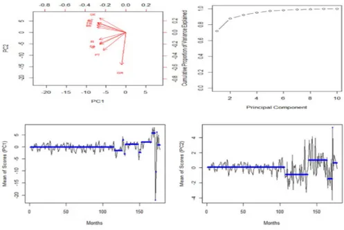
We found that PC1 and PC2, together, explain 88% of variance (see Fig. 1, top row; 72% by PC1 and 16% by PC2). It is worth noting that, apart from Greece, PC1 corresponds to a high correlation of bond yields. PC2 obviously corresponds to dif-ferentiation of bond yields as core and peripheral countries’ bond yields (top of zero belongs to core and bottom to peripheral). Among core countries, Austria and Neth-erlands are highly correlated, although, within peripheral countries, Italy and Spain are in a close relationship one with each other. As this component explicitly refers to economic powers of countries, Germany is in the strongest position and Greece is in the weakest. Such results seem therefore to be in line with the situation.
Bottom row of Fig. 1 shows means of scores on PC1 and PC2. Looking at the left plot, it is possible to note that PC1 dynamics do not change before the 150th
observation, which corresponds roughly to 2.5 years before the end of 2015. This implies that high correlation was valid for a very long time period. In contrast, dif-ferentiation emerges after the 100th observation on the right plot, which corresponds approximately to the date 2009:05. These results show, therefore, existence of some breakpoints for Euro area countries’ systemic co-movements in our sampling period. Using PELT method, we detected 11 change point locations for PC1 and 5 for PC2. Looking to bottom-right plot in Fig. 1, it can be said that the integrity of sovereign bond yields was maintained until 2010:08. Later, fluctuations became apparent with several lengths, and even monthly changes were observed.
The bottom-right plot which indicates differentiation of core and peripheral coun-tries, shows fewer change points and larger intervals. As we focused on disintegra-tion, we determined our sub-periods based on this information by combining the last four intervals in order to obtain enough observations for our future analysis and to simplify the process. Ultimately, we determine that bond yield co-movement levels haves changed significantly at following dates: 2009:11, 2012:07, and 2014:09.
Robustness Checks and Country Groups
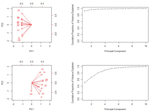
In order to test for significance of our sub-periods’ determination, we ran a PCA on bond yields for any sub-period identified. First time period (TP1) covers the sub-period from 2001:01 to 2009:10; second (TP2) from 2009:11 to 2012:06; third (TP3) from 2012:07 to 2014:08; finally fourth (TP4) from 2014:09 to 2015:12. For visualized relationships between bonds in different time intervals, see Figs. 2 and 3.
Fig. 2 The first two PCs for bond yields and cumulative proportion of variance explained by PCs (TP1-top row; TP2-bottom row)
For TP1, PC1 achieves an explanation rate of 92%, which represents an adequate score to rely on its significance alone. We can conclude that all bond yields are char-acterised by a strong correlation during this sub-period, which implies that TP1 can be defined as the pre-crisis period.
TP2 needs a deeper examination according to PCs’ scores. Loading scores for first four PCs and their explanation rates can be seen in Table 2. In this period, first two PCs suggest a break in common trends of yield movements, which can be
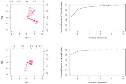
Fig. 3 The first two PCs for bond yields and cumulative proportion of variance explained by PCs (TP3-top row; TP4-bottom row)
Table 2 Loadings on the first four PCs of TP2 and their explanation rates Country PC1 PC2 PC3 PC4 Belgium (BE) 0.392 − 0.091 0.259 − 0.025 Germany (DE) 0.304 0.483 − 0.218 0.170 Ireland (IR) 0.277 − 0.190 − 0.423 − 0.376 Greece (GR) − 0.017 − 0.387 − 0.414 0.806 Spain (ES) 0.318 − 0.379 0.214 − 0.075 France (FR) 0.418 0.116 0.097 0.139 Italy (IT) 0.272 − 0.501 0.236 − 0.023 Netherlands (NL) 0.359 0.376 − 0.039 0.114 Austria (AU) 0.409 0.078 0.071 0.161 Portugal (PT) 0.174 − 0.133 − 0.646 − 0.339 Explanation Rate 51% 17% 13% 8%
attributed to a reduction in investor confidence on several countries, thus core and peripheral duality emerges. On PC2, gaps among countries become more evident, which conceivably relates to the fact that Germany and Netherlands were perceived as more secure economies whereas Spain, Italy, and Greece as the riskiest investing zones. It is not easy to read information provided by PC3, but it is possible to say that this component shows more complex divergence among countries. PC4 refers almost entirely to Greece bond yield movements. Thereby, it can be concluded that this period is highly associated with changing dynamics in Euro area countries. Thus, we called this period as the crisis period for Euro area.
For TP3, enough explanation rate (82%) is achieved with first two PCs (see Fig. 3). During the period, Belgium converges to other core countries and all strong economies tend to move together. PC2 loadings of countries whose economies suffer from sovereign debt problems are on same direction but, by considering both PC1 and PC2 loadings, it is not possible to say that these countries have high co-move-ments among themselves like core economies through this time period. Impacts of crisis are distinguishable. As this period still refers to a de-facto crisis phenomenon, we consider this period together with TP2 as the crisis period.
Finally, by examining first two PCs for TP4 (see Fig. 3), we can substantiate re-integration of core and peripheral countries except Greece with an explanation power of 82%. Distinctions are still observable among countries on PC2. The most notable point is that Greece is on in a very particular position compared to other countries on PC1 and PC2. This implies serious economic problems still observable for this country, and thus it deserves a more emphasis in order to understand reasons for this. Excluding Greece, we called this period as the post-crisis period for most Euro area countries, but it is not included in following analyses because it has too few observations for a reliable examination, specifically in VAR models.
These results are in line with Baur (2018) who found evidence of partially disin-tegrated Euro area bond markets during the debt crisis period, which is also seen as a necessary condition for strong contagion effects.
We built VAR models with groups of similar characteristics as found in here. Plots show clear evidence about these similar and different bond yield characteris-tics. Especially after pre-crisis period, groupings become obvious among Germany, France, Netherlands, Austria, Belgium (core) and among Portugal, Greece, Italy, Ireland, Spain (peripheral). Because Greece exhibits a distinct behaviour in periph-eral countries, we treat it as a third group itself in VAR models.
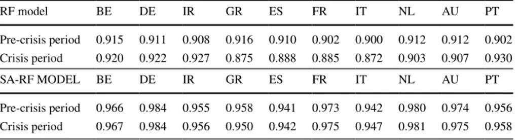
4.2 Random Forest Results and Simulated Annealing Algorithm Improvement
We ran RF models 20 times. Then, we calculated the average importance values of indicators and consulted rate of variance explained as the performance measure of the models. In Table 3 (RF Model part), the explanations for both pre-crisis and cri-sis periods are shown. Explanations are adequate for all countries but as explained before, a variable selection (also known as feature selection) technique is an ideal tool to overcome a high dimensional predictor space problem; as they foster learning by excluding irrelevant variables from the model. For this reason, we implemented
SA algorithm as a variable selection approach to find a near-optimal subset of predictors.
The enhanced learning performances achieved with the proposed variable selec-tion process can be seen in Table 3 (SA-RF part). The table shows improvement for both periods. We also conducted paired-samples t-test and non-parametric Mann–Whitney test to assess significance of explanation performances regarding to the base and the enhanced models. The hypothesis that mean explanation per-formance of the base model is equal to mean perper-formance of SA-RF model was rejected at 1% level of significance. Therefore, results from our model may conveni-ently be relied on.
4.2.1 Influencers of Bond Yields in Euro Area
Determinants of bond yields are selected according to the importance of variables given by RF models.
4.2.1.1 The Pre‑crisis Period Table 4 reports, for all countries, importance of the variables during the pre-crisis period and those selected for VAR models are under-lined. Looking at core countries, Belgium seems to be mostly influenced by Euro area unemployment, Euro area inflation, US unemployment, and the country’s own unemployment. Excluding Euro area inflation, the same influencers affected Ger-many, although US dollar rate played an influential role for Germany than Belgium. Influencing variables for Germany also had similar impacts on Netherlands. France bond yields was intensively related with country unemployment, whereas US unem-ployment and financial corporations’ debts had relatively minor effects. Among core countries, we found Brent oil price as one of primary influencers only for Austria, together with Euro area unemployment and financial corporations’ debts.
On the side of peripheral countries, some primarily influencing indicators are analogous to those affecting core countries and, we found that some market sen-timent variables were prominent. In particular, Ireland’s unemployment rate was the primary influencer for this country, followed by Euro area inflation, US unem-ployment, and Euro area industrial production. Greece had three high influencers, namely country GDP change rate, Euro area unemployment, and country economic sentiment indicator score. US dollar, Euro area inflation, country inflation, unem-ployment and government debt to GDP ratio change rates were main modifiers for
Table 3 Means of the variances explained by models
RF model BE DE IR GR ES FR IT NL AU PT Pre-crisis period 0.915 0.911 0.908 0.916 0.910 0.902 0.900 0.912 0.912 0.902 Crisis period 0.920 0.922 0.927 0.875 0.888 0.885 0.872 0.903 0.907 0.930 SA-RF MODEL BE DE IR GR ES FR IT NL AU PT Pre-crisis period 0.966 0.984 0.955 0.958 0.941 0.973 0.942 0.980 0.974 0.956 Crisis period 0.967 0.984 0.956 0.950 0.942 0.975 0.947 0.981 0.975 0.958
Table 4 V ar iable im por tance dur ing t he pr e-cr isis per iod Var iable BE DE IR GR ES FR IT NL AT PT countr y_ESI 4.391 4.583 9.124 7.267 4.604 CONS_countr y_C OF 3.897 7.411 7.596 13.588 countr y_Debt.GDP_Chang e 7.497 4.473 6.913 8.332 9.901 7.659 6.278 6.897 countr y_Inflation 3.788 7.662 10.042 8.666 8.588 countr y_U nem plo yment 9.653 13.113 11.897 11.670 16.573 11.541 11.799 10.207 countr y_GDP_Chang e 6.100 7.705 13.445 5.372 7.451 4.683 countr y_T ot al_Cr edit_t o_Go ver ment.GDP_Chang e 2.646 4.138 6.208 5.617 4.207 countr y_S toc k_R etur ns 0.417 0.604 countr y_GDP .Capit a_Chang e 3.271 4.747 7.439 5.346 EA_ESI 5.126 6.024 5.005 6.456 4.396 6.291 6.090 5.345 Eur opean_N ew s_Inde x 2.259 5.800 6.364 CONS_EA_C OF 7.060 4.667 6.527 7.182 8.340 US_Dollar 8.691 6.621 16.146 8.590 10.727 11.509 EA_Inflation 10.864 5.099 8.580 13.608 14.167 6.990 8.670 11.863 US_U nem plo yment 9.639 10.556 8.489 6.203 8.028 9.952 10.384 11.347 EA_U nem plo yment 16.754 11.222 6.657 11.659 8.539 10.208 16.708 17.675 Financial_Cor por ations_Debt 8.387 7.994 6.779 9.165 10.343 K ansas_City_F inancial_S tress 7.760 7.913 8.339 8.302 6.165 7.369 7.633 Eur ope_Br ent_Oil_Pr ice 7.050 7.065 10.736 10.606 EA_Indus trial_Pr oduction 5.861 8.131 8.084 8.099 6.934 6.411 6.687 EUS TO XX_R etur ns 1.014 − 0.611 1.568 − 0.163 US_S toc k_R etur ns 0.964 0.579 1.266 0.502 W or ld_GDP_Chang e 3.187 6.411 7.469 8.042 EA_GDP_Chang e 6.045 6.840 7.013
Var iable BE DE IR GR ES FR IT NL AT PT Int_Bank_Clms_on_Bank s.GDP_Chang e 4.128 3.597 3.909 Int_Bank_Clms_on_N on.Bank s.GDP_Chang e 4.142 2.842 4.745 4.020 6.065 5.124 Table 4 (continued)
bond yields in Spain. Italy had five remarkable influencers: Country unemployment rate, US dollar rate, Euro area inflation, Euro area unemployment, and Brent oil price. Lastly, consumer confidence indicator, country and US unemployment rates, and Euro area inflation rate were found as directive variables for Portugal.
4.2.1.2 The Crisis Period Table 5 reports, for all countries, importance of the vari-ables during the crisis period and those selected for VAR models are underlined. Fundamental variables that affected core countries during the pre-crisis period seem preserved their relevance during the crisis period. Euro area inflation and unemploy-ment rates, US dollar rate, and US unemployunemploy-ment rate were noteworthy for Belgium. Euro area unemployment was determinant for all core countries, especially for Neth-erlands with its high importance value. Country unemployment rate was mutually important for Germany, France, Netherlands, and Austria. US unemployment was the other primary influencer for bond yields in both Germany and Austria. France, Netherlands, and Austria were under the influence of US dollar. Country GDP change rate was another relevant variable for Austria, whereas country economic sentiment indicator seems to be the only market sentiment variable that had a notable effect on Netherlands.
Looking at peripheral countries, country unemployment rate, GDP change, and US unemployment represented three primary influencers for Ireland where they exerted increased effects on the bond yields compared to the pre-crisis period. Greece received higher exposure to country economic sentiment indicator, country government debt to GDP ratio change, and Euro area inflation. Together with these, Euro area unemployment rate exerted a relevant influence on bond yields in Greece. Spain and Italy had more primary influencers than other countries. Country govern-ment debt to GDP change and country inflation, US dollar, Euro area inflation and Euro area industrial production were the most significant bond yields’ influencers in Spain; also, as a market sentiment indicator, Kansas City Financial Stress score was found to be high. Country unemployment and Euro area inflation rates were important for both Italy and Portugal. US dollar rate, US and Euro area unemploy-ment rates, and World GDP change rate were remaining noteworthy determinants for Italy, and country GDP change, consumer confidence indicator, and Kansas City Financial Stress score were in the foreground for Portugal. Selected variables to include in VAR models in next step are summarized in Appendix C.
4.3 Vector Autoregression Models’ Results and Simulated Annealing Algorithm Improvement
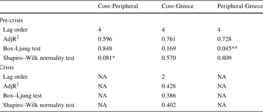
Key performance measures of VAR models are shown in Table 6. Tests suggest that for both crisis and crisis periods, only Core-Greece models are adequate. In pre-crisis period, other models’ diagnostics failed to validate appropriateness of mod-els but especially in crisis period, modmod-els have series problems. These problems are mainly due to low number of observations against total number of variables with their lags included in models.
Table 5 V ar iable im por tance dur ing t he cr isis per iod Var iable BE DE IR GR ES FR IT NL AT PT countr y_ESI 5.098 5.024 10.771 7.246 9.760 4.608 6.625 CONS_countr y_C OF 5.605 13.401 countr y_Debt.GDP_Chang e 6.371 5.109 7.506 10.825 10.224 7.082 7.039 countr y_Inflation 7.092 10.470 6.249 7.932 4.834 countr y_U nem plo yment 13.542 13.967 12.920 10.736 10.742 10.501 9.550 countr y_GDP_Chang e 6.127 10.756 8.641 4.338 5.754 9.421 9.927 countr y_T ot al_Cr edit_t o_Go ver ment. GDP_Chang e 4.371 5.283 4.042 countr y_S toc k_R etur ns 0.300 1.494 1.825 countr y_GDP .Capit a_Chang e 5.448 8.914 7.464 4.929 5.556 5.385 8.142 EA_ESI 5.898 5.678 4.493 5.527 5.813 6.000 Eur opean_N ew s_Inde x 3.927 4.863 5.752 5.338 CONS_EA_C OF 7.108 5.475 6.747 US_Dollar 10.413 7.035 15.887 9.303 9.626 9.516 9.503 6.404 EA_Inflation 12.044 5.571 10.849 15.000 6.114 14.627 6.683 7.189 13.025 US_U nem plo yment 10.534 12.042 9.181 8.738 8.638 9.439 9.901 EA_U nem plo yment 15.736 11.942 8.211 13.918 8.039 11.578 9.255 18.349 15.215 Financial_Cor por ations_Debt 8.485 7.441 8.017 K ansas_City_F inancial_S tress 7.996 7.225 9.224 7.403 4.941 9.192 Eur ope_Br ent_Oil_Pr ice 9.174 6.242 7.974 EA_Indus trial_Pr oduction 8.729 9.623 7.365 7.016 6.193 7.857 EUS TO XX_R etur ns 1.400 0.074 US_S toc k_R etur ns 0.864 0.874 0.958 W or ld_GDP_Chang e 7.633 6.638 7.011 11.005 5.784 EA_GDP_Chang e 6.484 5.545 4.077 6.590 5.503 4.886
Var iable BE DE IR GR ES FR IT NL AT PT Int_Bank_Clms_on_Bank s.GDP_Chang e 3.576 3.357 6.492 Int_Bank_Clms_on_N on.Bank s.GDP_ Chang e 4.219 5.437 4.005 6.153 3.503 3.786 Table 5 (continued)
After SA algorithm was used for variable selection, better results are achieved, and high-dimension problem have overcome. Results are shown in Table 7. In next step, variables with significant impacts on spreads are considered and presented only.
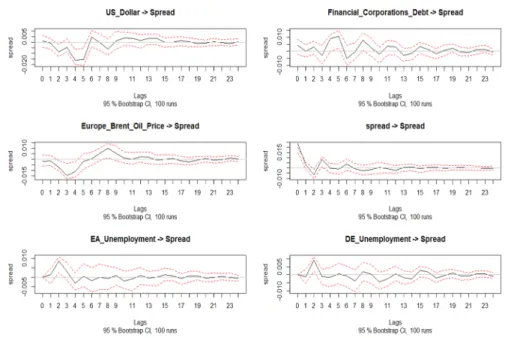
4.3.1 Contagion in Euro Area
4.3.1.1 The Pre‑crisis Period Reaction of Core-Peripheral groups’ bond yield spread to shocks in selected variables’ can be seen in Fig. 4. IRFs indicate that most sig-nificant effects are emerged from shocks in US Dollar, Brent Oil Price, Spread’s own innovations, EA Unemployment and DE Unemployment. Shocks in Spread has instant and high positive impact on itself, which turns to negative and become posi-tive again within few lags. US Dollar shocks have negaposi-tive significant responses on spread after two periods and this effect fades off after six periods. Like US Dollar,
Table 6 Key performance measures of VAR models with all determinant variables
*Significant at the 10% level **Significant at the 5% level
Core-Peripheral Core-Greece Peripheral-Greece Pre-crisis
Lag order 4 4 4
AdjR2 0.596 0.761 0.728
Box-Ljung test 0.848 0.169 0.045**
Shapiro–Wilk normality test 0.081* 0.570 0.809
Crisis
Lag order NA 2 NA
AdjR2 NA 0.428 NA
Box–Ljung test NA 0.386 NA
Shapiro–Wilk normality test NA 0.402 NA
Table 7 Key performance measures of VAR-SA models with selected variables
Core-Peripheral Core-Greece Peripheral-Greece Pre-crisis
Lag order 4 4 4
AdjR2 0.688 0.788 0.739
Box–Ljung test 0.552 0.528 0.480
Shapiro–Wilk normality test 0.699 0.531 0.842
Crisis
Lag order 2 2 2
AdjR2 0.321 0.582 0.659
Box–Ljung test 0.587 0.153 0.449
Brent Oil Price shocks have negative significant responses on spread between lags two and four and at lag eight, a positive impact becomes evident. Oil Price’s effect then declines to zero sharply. Shocks in Financial Corporations’ Debt have positive impact on spread through four and five period lags. Beside these, significant shock effects emerge at some lags; negatively from ES Debt to GDP Ratio at lag 4 and posi-tively from EA Unemployment and DE Unemployment shocks at lag two.
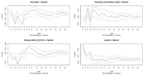
Impulse response plots of core-Greece groups’ bond yield spreads with selected variables are shown in Fig. 5. US Dollar and Brent Oil Prices impacts follow very similar patterns to core-peripheral ones. Significant negative impacts are observed at lag lags two and five from US Dollar and after first period to fourth period for Brent Oil Price, which eventually turned to positive impact for eight and ninth lags. Spread shocks have positive responses which begin instantly and continues until fourth lag. Financial Corporations’ Debt causes significant positive responses on spread at lags two and five.
Impulse response plots of Peripheral-Greece groups’ bond yield spreads with selected variables are shown in Fig. 6. Again, for Peripheral-Greece bond yield spreads, Brent Oil Price shocks have similar response pattern like in previous two groups. As observed in core-Greece spreads, Spread shocks have gradually decreas-ing positive impacts until third period. ES Debt to GDP Ratio Change shocks effect spread positively at lag two. Unemployment rates in IR and PT have significant neg-ative impacts on spread at lag one.
Broadly, it is possible to say that spreads against core countries’ bond yields are more sensitive to US Dollar, Financial Corporations’ Debt and Brent Oil Price. Latter one is also an important contagion factor for Peripheral-Greece bond yield
spreads. Spread is found as the most effective shock source on all three group spreads.
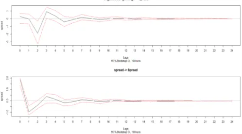
4.3.1.2 The Crisis Period Industrial production and inflation in EA,
unemploy-ment rates in IR and IT and spread’s own shocks have significant impacts on bond yield spreads between core and peripheral groups in crisis period (see Fig. 7).
Fig. 5 Core countries-Greece bond yield spread responses to shocks in pre-crisis period
Industrial production has a negative significant effect at first lag which then rapidly converges to zero. Shocks in EA Inflation have significant positive responses on spread after first period until third period. Both unemployment rates have positive impacts on spread at first lag. Spread’s own shocks have an instant and strong posi-tive impact on itself; but shocks are no longer effecposi-tive after first period.
Core economies-Greece contagion (see Fig. 8) is triggered by short term pow-erful shocks of GR Debt to GDP Ratio Change at lags two with negative response and Spread’s own shocks with positive response emerging instantly which turns into negative response for lags one and two.
GR Debt to GDP Ratio Change shocks and Spread’s owns shocks effect periph-eral countries-Greece bond yield spreads likewise core economies-Greece bond yield spreads (see Fig. 9). Beside these two, PT Unemployment has a positive impact on spread at lag two, which then loses its significance and settles around zero after eight period.
In the crisis period, number of transmission channels have seen decreased and shocks are significant only at short lags. This points to disintegration of EA coun-tries during the crisis time and possible proactive strategies to prevent adverse effects to spread. An important finding is that between Greece and other groups, magnitude of impacts is very high. Together with Step 1 findings, Greece is found in an opted-out position among EA.
5 Conclusions
The 2008 US sub-prime crisis has been remarkable in its severity and has raised many concerns about the problem of contagion in financial markets. In particular, the risk of large shock transmissions in sovereign default has driven policymakers to invoke necessity of bailouts aimed at containing the negative effects resulting from shock
Fig. 8 Core countries-Greece bond yield spread responses to shocks in crisis period
propagation. In this context, understanding the determinants of financial contagion can be particularly relevant for policymakers to take corrective actions and investors to implement preventive hedging strategies and eventually design the most suitable crisis management policies. Shedding light on the contagion determinants may be useful for investors who can derive relevant information about countries which are less sensitive to be affected by shocks, orienting thus their investment strategies.
Major challenge of such examinations is their complex nature; there are too many candidate variables and it is not an easy -and sometimes impossible- task to form proper models and obtain consistent results. Instead of making subjective modelling decisions, which are mostly based on prior knowledge and/or intuitions, implementing machine learning methods without any restrictions possess more opportunities in terms of information revealing from data. Besides, more meaningful and reliable outputs can be reached by using metaheuristic optimization algorithms for variable selection.
In this framework, the present study has contributed to the empirical literature on contagion by investigating the determinants of shocks propagation in the Euro area with optimized learning and econometric models, using data for the period 2001–2015 from ten EMU countries (five core economies and five peripheral countries). First part of our analysis show that Greece must be considered as a separate country than other peripheral countries due to its government bond yield’s distinct behaviour.
Overall, our analysis indicates that innovations in bond yield spreads between groups represents the most significant source of shock propagation in the Euro Area and that other global indicators—especially US dollar/Euro exchange rate, Financial Corpora-tion’s Debts and Brent Oil Price—form the most relevant subset in increasing the prob-ability of a contagious event. In contrast our findings reveal a less relevant role played by macroeconomic fundamental variables in attracting bear market speculative attacks that could generate financial tensions upon the public accounts, short selling strategies on public securities and consequently increase the risk of contagion. It is worth noting that the economic literature has suggested other possible determinants of shock propa-gation in addition to those considered in this article, such as changes in risk aversion or an updating of creditors’ beliefs about the likelihood of a sovereign default. Therefore, further lines of research could assess these other channels so that policymakers can be fully informed about the potential externalities from a sovereign default. Finally, our findings could induce to analyse in detail the risk of contagion resulting from specula-tive strategies of institutional investors, above all in those countries or areas with struc-tural weaknesses that therefore may significantly suffer from a speculative attack, as happened in several EMU countries in recent years.
Appendix A: Details on Variables
US_Dollar US dollar exchange rate against Euro. Monthly averages
ESI Composite statistical indicator in order to quantify overall economic activity based on the results from business surveys about current economic situation and expectations about future developments of different sectors
CONS_COF Consumer confidence indicator about current economic situation and expectations about future developments
Debt_GDP_Change Yearly change rate of the ratio that is the amount of a country’s total gross government debt as a percentage of its GDP. The same change rate was used for all months of corresponding year
Inflation Yearly inflation rate. A harmonised index of consumer prices was used as inflation measure. The rate used was the same for all months of the corresponding year
GDP_Capita_Change Yearly change rate of Gross Domestic Product per capita. The change rate used was the same for all months of corresponding year Unemployment Harmonised unemployment rate that defines the unemployed as people
of working age who are without work, are available for work, and have taken specific steps to find work
Int_Bank_Clms_on_Banks/
Non-Banks_GDP_Change Banks’ cross-border claims denominated in all currencies plus their local claims denominated in foreign currencies to global GDP ratio changes. They were used as “global liquidity” indicators. Data were quarterly; the change rate used was the same for all months of the corresponding quarter
Total_Credit_to_Government
GDP_Change Credit to the general government sector to GDP ratio quarterly change rate. Instruments included are currency and deposits; loans; debt securities. The change rate used was the same for all months of the corresponding quarter
Debt Indebtedness of private sector in Europe. Three sectors were used: banks, non-financial corporations and households
European_Brent_Oil_Price Spot price of oil, which is a blended crude stream produced in the North Sea region and that serves as a reference or "marker" for pricing a number of other crude streams
Industrial_Production The output of industrial establishments; this covers sectors such as min-ing, manufacturing and public utilities (electricity, gas and water) GDP_Change Yearly GDP change. The change rate used was the same for all months
of the corresponding year
EU_News_Index European policy-related economic uncertainty, an index based on news-paper articles regarding policy uncertainty developed by (Baker et al. 2016). The higher the value, the more the uncertainty
Returns Monthly stock market returns of countries. Closing value of the month was used. Benchmark indexes: BEL20 (Belgium), CAC40 (France), DAX (Germany), ISEQ20 (Ireland), FTSE MIB (Italy), AEX (Neth-erlands), IBEX35 (Spain), ATX (Austria), PSI 20 (Portugal), ATHEN INDEX COMPOS (Greece)
EUSTOXX_Returns Monthly Euro area stock returns. ESTX 50 index is used as benchmark. Closing value of the month was used
Kansas_City_Financial_Stress The Kansas City Financial Stress Index. This is a monthly measure of stress in the US financial system based on 11 financial market variables. A positive value indicates that financial stress is above the long-run average, while a negative value signifies that financial stress is below the long-run average
Appendix C: Selected Variables for Each Group, According to SA‑RF Results
Pre-crisis period
Core Peripheral Greece
BE_Unemployment IR_Unemployment GR_ESI
EA_Unemployment US_Unemployment GR_GDP_Change
DE_Unemployment ES_Unemployment EA_Unemployment
FR_Unemployment IT_Unemployment NL_Unemployment EA_Unemployment US_Unemployment PT_Unemployment EA_Inflation EA_Inflation US_Dollar ES_Inflation Financial_Corporations_Debt US_Dollar Europe_Brent_Oil_Price EA_Industrial_Production ES_Debt.GDP_Change Europe_Brent_Oil_Price CONS_PT_COF Crisis period:
Core Peripheral Greece
EA_Unemployment IR_Unemployment
DE_Unemployment US_Unemployment GR_ESI
FR_Unemployment PT_Unemployment GR_Debt.GDP_Change
NL_Unemployment EA_Unemployment EA_Unemployment
US_Unemployment IT_Unemployment EA_Inflation
AT_Unemployment IR_GDP_Change NL_ESI PT_GDP_Change EA_Inflation US_Dollar US_Dollar ES_Inflation EA_Inflation EA_Industrial_Production ES_Debt.GDP_Change Kansas_City_Financial_Stress CONS_PT_COF World_GDP_Change
Appendix D: Considered VAR Equations for Pre‑crisis and Crisis Periods
where D denotes the vector of selected variables given in Appendix C, β the vector of variable coefficients, m the lag order and ϵt is an unobservable zero mean white noise vector process. It is worth noting that IRFs are created after SA improvement, which also lowers the number of included variables.
Funding Open access funding provided by Università di Foggia within the CRUI-CARE Agreement.
Data availability All data employed in the manuscript are available on request.
Declarations
Conflict of interest The authors declare that they have no conflict of interest.
Open Access This article is licensed under a Creative Commons Attribution 4.0 International License, which permits use, sharing, adaptation, distribution and reproduction in any medium or format, as long as you give appropriate credit to the original author(s) and the source, provide a link to the Creative Com-mons licence, and indicate if changes were made. The images or other third party material in this article are included in the article’s Creative Commons licence, unless indicated otherwise in a credit line to the material. If material is not included in the article’s Creative Commons licence and your intended use is not permitted by statutory regulation or exceeds the permitted use, you will need to obtain permission directly from the copyright holder. To view a copy of this licence, visit http://creat iveco mmons .org/licen ses/by/4.0/.
References
Acemoglu D, Ozdaglar A, Tahbaz-Salehi A (2015) Systemic risk and stability in financial networks. Am Econ Rev 105(2):564–608
Allen F, Babus A, Carletti E (2009) Financial crises: theory and evidence. Annu Rev Financ Econ 1(1):97–116
Apergis N (2015) Forecasting Credit Default Swaps (CDSs) spreads with newswire messages: evi-dence from European countries under financial distress. Econ Lett 136:92–94
(7)
Core − Peripheral Spreadt= j=m ∑
j=1
𝛽jCore − Peripheral Spreadt−j+ j=m ∑
j=1
𝜷jDt−j+ 𝜖t
(8)
Core − Greece Spreadt= j=m ∑ j=1
𝛽jCore − Greece Spreadt−j+ j=m ∑ j=1
𝜷jDt−j+ 𝜖t
(9) Peripheral − Greece Spreadt=
j=m
∑
j=1
𝛽jPeripheral − Greece Spreadt−j+
j=m
∑
j=1
Athey S (2018) The impact of machine learning on economics. In: Agrawal A, Gans J, Goldfarb A (eds) The economics of artificial intelligence: an agenda, pp 507–552. https ://doi.org/10.7208/ chica go/97802 26613 475.003.0021
Athey S, Imbens GW (2019) Machine learning methods that economists should know about. Annu Rev Econ 11(1):685–725. https ://doi.org/10.1146/annur ev-econo mics-08021 7-05343 3
Baker SR, Bloom N, Davis SJ (2016) Measuring economic policy uncertainty. Q J Econ 131(4):1593–1636
Baum CF, Schäfer D, Stephan A (2016) Credit rating agency downgrades and the Eurozone sovereign debt crises. J Financ Stab 24:117–131
Baur DG (2018) Decoupling and contagion: the special case of the eurozone sovereign debt crisis. Int Rev Finance. https ://doi.org/10.1111/irfi.12220
Becker B, Hall SG (2012) Spurious common factors
Bernal O, Gnabo J-Y, Guilmin G (2016) Economic policy uncertainty and risk spillovers in the Euro-zone. J Int Money Financ 65:24–45
Billio M, Pelizzon L (2003) Contagion and interdependence in stock markets: have they been misdi-agnosed? J Econ Bus 55(5):405–426
Boumparis P, Milas C, Panagiotidis T (2015) Has the crisis affected the behavior of the rating agencies? Panel evidence from the Eurozone. Econ Lett 136:118–124
Bratis T, Laopodis NT, Kouretas GP (2015) Creditor moral hazard during the EMU debt crisis. J Int Financ Mark Inst Money 39:122–135
Broto C, Perez-Quiros G (2015) Disentangling contagion among Sovereign CDS spreads during the European debt crisis. J Empir Financ 32:165–179
Brutti F, Sauré P (2015) Transmission of sovereign risk in the euro crisis. J Int Econ 97(2):231–248 Calvo GA, Mendoza EG (2000) Rational contagion and the globalization of securities markets. J Int Econ
51(1):79–113
Calvo SG, Reinhart CM (1996) Capital flows to Latin America: is there evidence of contagion effects? Caporin M, Pelizzon L, Ravazzolo F, Rigobon R (2018) Measuring sovereign contagion in Europe. J
Financ Stab 34:150–181. https ://doi.org/10.1016/j.jfs.2017.12.004
Corsetti G, Pericoli M, Sbracia M (2005) ‘Some contagion, some interdependence’: more pitfalls in tests of financial contagion. J Int Money Financ 24(8):1177–1199
Corsetti G, Pesenti P, Roubini N, Tille C (2000) Competitive devaluations: toward a welfare-based approach. J Int Econ 51(1):217–241
Cronin D, Flavin TJ, Sheenan L (2016) Contagion in Eurozone sovereign bond markets? The good, the bad and the ugly. Econ Lett 143:5–8
Dickey DA, Fuller WA (1979) Distribution of the estimators for autoregressive time series with a unit root. J Am Stat Assoc 74(366):427–431
Drazen A (2000) Political contagion in currency crises. In: Currency crises. University of Chicago Press, pp 47–67
Dufrénot G, Gente K, Monsia F (2016) Macroeconomic imbalances, financial stress and fiscal vulnerabil-ity in the euro area before the debt crises: a market view. J Int Money Financ 67:123–146
Forbes KJ, Rigobon R (2002) No contagion, only interdependence: measuring stock market comove-ments. J Financ 57(5):2223–2261
Gai P, Kapadia S (2010) Contagion in financial networks. Proc R Soc Lond A Math Phys Eng Sci 466(2120):2401–2423
Gai P, Haldane A, Kapadia S (2011) Complexity, concentration and contagion. J Monet Econ 58(5):453–470
Gerlach S, Smets F (1995) Contagious speculative attacks. Eur J Polit Econ 11(1):45–63
Gilli M, Winker P (2008) A review of heuristic optimization methods in econometrics. Swiss Finance Institute Research, 08–12
Goldstein M, Kaminsky GL, Reinhart CM (2000) Assessing financial vulnerability: an early warning system for emerging markets. Peterson Institute
Gómez-Puig M, Sosvilla-Rivero S (2016) Causes and hazards of the euro area sovereign debt crisis: pure and fundamentals-based contagion. Econ Model 56:133–147
Helbing D (2012) Agent-based modeling. In: Social self-organization . Springer, pp 25–70
Ho SH (2016) Long and short-runs determinants of the sovereign CDS spread in emerging countries. Res Int Bus Financ 36:579–590
Kaminsky GL, Reinhart CM (2000) On crises, contagion, and confusion. J Int Econ 51(1):145–168 Kaminsky GL, Reinhart C (2003) The center and the periphery: the globalization of financial turmoil
Kaminsky GL, Reinhart CM, Vegh CA (2003) The unholy trinity of financial contagion. J Econ Perspect 17(4):51–74
Kaufman GG (1992) Bank contagion: theory and evidence (No. 92-13). Federal Reserve Bank of Chicago Killick R, Fearnhead P, Eckley IA (2012) Optimal detection of changepoints with a linear computational
cost. J Am Stat Assoc 107(500):1590–1598. https ://doi.org/10.1080/01621 459.2012.73774 5 Koop G, Korobilis D (2016) Model uncertainty in panel vector autoregressive models. Eur Econ Rev
81:115–131
Kwiatkowski D, Phillips PCB, Schmidt P, Shin Y (1992) Testing the null hypothesis of stationarity against the alternative of a unit root: how sure are we that economic time series have a unit root? J Econom 54(1–3):159–178
Lansangan JRG, Barrios EB (2009) Principal components analysis of nonstationary time series data. Stat Comput 19(2):173–187. https ://doi.org/10.1007/s1122 2-008-9082-y
Liaw A, Wiener M (2002) Classification and regression by RandomForest. R News 2(3):18–22
Longstaff FA (2010) The subprime credit crisis and contagion in financial markets. J Financ Econ 97(3):436–450
Masson PR (1998) Contagion: monsoonal effects, spillovers, and jumps between multiple equilibria, pp 1–32
Masson PR (1999) Contagion: macroeconomic models with multiple equilibria. J Int Money Financ 18(4):587–602
Mondria J, Quintana-Domeque C (2013) Financial contagion and attention allocation. Econ J 123(568):429–454
Núñez F, Usabiaga C (2008) Introducing VAR and SVAR predictions in system dynamics models. In: Onatski A, Wang C (eds) Int. J. simulation and process modelling, vol 4. CEMFI, Madrid. Spurious Factor Analysis (No. 2020/01)
Pfaff B (2008) VAR, SVAR and SVEC models: implementation within {R} package {vars}. J Stat Softw 27(4)
Pragidis IC, Aielli GP, Chionis D, Schizas P (2015) Contagion effects during financial crisis: evidence from the Greek sovereign bonds market. J Financ Stab 18:127–138
Pyndyck RS, Rubinfeld DL (1991) Econometric models and economic forecasts. McGraw Hill, New York
Rigobon R (2016) Contagion, spillover and interdependence. European Central Bank Working Paper Series No. 1975
Siebenbrunner C, Sigmund M, Kerbl S (2017) Can bank-specific variables predict contagion effects? Quant Financ 17(12):1805–1832
Sims CA (1980) Macroeconomics and reality. Econometrica, 1–48.
Singh MK, Gómez-Puig M, Sosvilla-Rivero S (2016) Sovereign-Bank linkages: quantifying directional intensity of risk transfers in EMU countries. J Int Money Financ 63:137–164
Smaga P (2014) The concept of systemic risk. Systemic Risk Centre Special Paper, 5
Upper C (2011) Simulation methods to assess the danger of contagion in interbank markets. J Financ Stab 7(3):111–125
Wager S, Athey S (2018) Estimation and inference of heterogeneous treatment effects using random for-ests. J Am Stat Assoc 113(523):1228–1242. https ://doi.org/10.1080/01621 459.2017.13198 39
Publisher’s Note Springer Nature remains neutral with regard to jurisdictional claims in published maps and institutional affiliations.