A MULTI FOCI CLOSED CURVE: CASSINI OVAL, ITS
PROPERTIES AND APPLICATIONS
ÇOK MERKEZLİ KAPALI BİR EĞRİ: CASSİNİ OVALİ, ÖZELLİKLERİ VE UYGULAMALARI
Mümtaz KARATAŞ
Naval Postgraduate School, Operations Research Department [email protected]
ABSTRACT: A Cassini oval is a quartic plane curve defined as the set (or locus) of
points in the plane such that the product of the distances to two fixed points is constant. Its unique properties and miraculous geometrical profile make it a superior tool to utilize in diverse fields for military and commercial purposes and add new dimensions to analytical geometry and other subjects related to mathematics beyond the prevailing concept of ellipse. In this study we explore and derive analytical expressions for the properties of these curves and give a summary of its applications with distinct examples.
Keywords: Cassini Ovals; Multi Foci Curves JEL Classification: C65; C60
ÖZET: Cassini ovali, düzlem üzerindeki sabit iki noktaya olan mesafelerinin
çarpımı yine bir sabit olan noktalar kümesinin oluşturduğu kuadratik bir eğri olarak tanımlanabilir. Benzersiz özellikleri ve geometrik profili, bu ovalleri pek çok askeri ve ticari alanda kullanılmasına imkan tanıyan üstün bir araç haline getirmiş, ayrıca analitik geometriye ve genel elips konseptinin ötesindeki matematik teorisiyle ilişkili diğer konulara yeni bir boyut kazandırmıştır. Bu çalışma kapsamında, Cassini ovallarinin çeşitli özellikleriyle ilgili analitik ifadeler geliştirilmiş ve farklı alanlardan örnekler kullanılarak söz konusu ovallerin uygulama alanlarına ilişkin özet bilgi verilmiştir.
Anahtar Kelimeler: Cassini Ovalleri; Çok Merkezli Eğriler
1. Introduction
Curves in the plane that arise as the set of solution points of equations have been studied for hundreds of years, some going back to ancient Greece. Some of the more interesting examples have been studied in great detail and a lot is known about them. The purpose of this paper is to convey a small amount of the vast body of knowledge amassed over the centuries about the Cassini ovals in the plane in terms of geometrical properties and application areas.
Ovals of Cassini (or the Cassinian Ovals) were first studied in 1680 by Giovanni Domenico Cassini (1625–1712, aka Jean-Dominique Cassini) as a model for the orbit of the Sun around the Earth (Gibson, 2007). He discovered four satellites of Saturn and made measurements of the rotation periods of Mars and Jupiter. He then rejected the theory of Kepler ellipses and Roemer’s theory and he discovered the so-called Cassini ovals suggesting that stellar bodies followed paths traced out by one of these curves (Sivardiere, 1994; Gillespie, 1971, Glenn, Littler 1984, The New Encyclopedia Britannica, 1987). Other names include Cassinian ovals, Cassinian
curves and ovals of Cassini. These curves are characterized in such a way that the product of the distances from two fixed focal points F1 and F2 is constant b2 (while
for a normal ellipse the sum of the distance of two fixed focal points is constant) and the distance (F1,F2)=2a (Hellmers, Eremina, Wriedt, 2006). Therefore it is possible
to express a Cassini oval by using the parameters a and b where a is the semi-distance between the two foci and b is the constant which determines the exact shape of the curve as will be discussed later. In (James, James, 1949) a Cassini oval is defined as “the locus of the vertex of a triangle when the product of the sides adjacent to the vertex is a constant and the length of the opposite side is fixed”. The curve is symmetrical about the x-axis as well as the y-axis. So it is sufficient to generate the first quadrant of the coordinate system and use reflection about the x-axis and the y-axis to generate the other three parts (Ray, Ray, 2011).
Besides being a model for the orbit of planets, Cassinian curves are also used in various scientific applications such as nuclear physics, biosciences, acoustics, etc. Its unique properties and miraculous geometrical profile make it a superior tool to utilize in diverse fields for military and commercial purposes. Being an interesting curve makes it to be much better known than it is. In this study our main ambition is to explore some of the useful properties of these curves, derive analytical expressions for its area, perimeter, convex hull and interior cover and give a summary of its applications in science and commerce with distinct examples. We start with a short and formal description of the Cassini ovals and its Cartesian and polar equations. This is followed by an overview of the useful properties continued by the derivation of its area, perimeter, convex hull and interior cover together with some approximations rarely given in the literature. Next we present an overview of the applications in nuclear physics, biosciences, demography, acoustics, military, commerce, etc. Finally we give a summary and conclusions.
2. Cassinian Oval Properties
2.1. Oval Equations
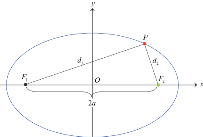
The Cassini ovals are defined in two-center bipolar coordinates by the equation below:
2 1 2
d d b (1)
where d1 and d2 denote the ranges F1 to P and P to F2 respectively as in Figure 1. If
we locate the origin (0,0) of Cartesian plane at the midpoint of the two foci F1 and
F2, and choose the x-axis as the line joining them, then the foci will have the
coordinates (±a,0). The F1, P and F2 triangle is sometimes called as the “bistatic
triangle” to describe the sensor-target geometry especially in military applications of the ovals that will be discussed in Chapter 3. The Cassini ovals have the following quadratic polynomial Cartesian equation:
2 2 2 2 4
(x a) y (x a) y b a b, , .
Figure 1. A Cassini oval with foci F1 and F2 on the x-axis
Since substituting -x for x and/or –y for y does not change the equality (2), the above curve is symmetric with respect to both axis and origin. Next let us convert the equation to one in polar coordinates. Let x=r.cosθ and y=r.sinθ so that x2y2 r2. Then we have;
4 2 2 2cos(2 ) 4 4 0
r a r a b (3)
2 2cos 2 4cos (2 ) (2 4 4)
r a a a b (4)
which means for r,
4 2 cos(2 ) b sin (2 ) r a a (5)
There are two conventions for r in polar coordinates: i) that r be nonnegative, ii) that it can take any real value. For the first alternative it ties in strongly with complex numbers, but it lacks in describing the curve smoothly in all cases (Hirst, Lloyd, 1997). To remedy the situation we will restrict θ so that the radicand will be greater than or equal to zero. To do this we define 0
as in (6)
:2 2 1 0 1 sin(2 ) sin 2 b b a a (6)
Assuming that negative values of r are redundant and restricting (5) to the case where x y 1 d d2 O 2a P 1 F 2 F
0 0 [ , ] and 2 1 0 1 sin 2 b a . the parametric formula for the oval becomes:
cos( ),sin( )
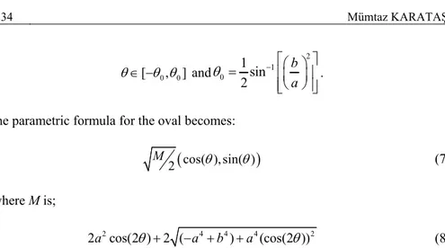
2 M (7) where M is; 2 4 4 4 2 2 cos(2 ) 2 (a a b )a (cos(2 )) (8) with 0<θ<2π and a<b. The parameterization only generates parts of the curve whena>b.
2.2. Cassini Shapes
The Cassini shape depends on the parameters a and b and is generally categorized by evaluating the ratio a/b. In Figure 2 are drawn Cassini ovals for fixed a on the left and fixed b on the right.
Figure 2. A family of Cassini Ovals
The form of the ovals can be characterized as follows:
For a b 2 2 the curve is a single loop that looks like an ellipse and intersects x-axis at x a2b2 .
For 2 2a b1 the oval attains a dent on top and bottom (peanut-shaped).
When a/b=1 the curve is a Lemniscate of Bernoulli (in Latin lemniscates means “adorned with ribbons”) which has a point of self intersection. This shape passes through the origin has a shape similar to the ∞ symbol. For a/b>1 the curve splits into two mirror-imaged disjoint ovals and there
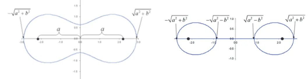
In Figure 3 are the intersection points on x-axis for a/b<1 and a/b>1 cases. For the a/b>1 case, there are two additional real x-intercepts.
Figure 3. Real x-intercepts for a/b<1 and a/b>1 cases
Looking at Figure 2 and Figure 3 we can come up with some other useful properties of the Cassini ovals such as the least thickness, 2 b2a2 , greatest thickness, b a , 2 and diameter, 2 a2b2 . One other property of a special case of Cassini oval, the Lemniscate of Bernoulli, is that the curve is also described by the equation;
2 2cos(2 )
r a (9)
Equation (9) is defined for
4, 4
and
3 4,5 4
.2.3. Area of a Cassini Oval
The area of a Cassini oval, AC, can be reduced to a single numerical integration as
follows. Since the oval is symmetric with respect to both axes we can compute AC
by multiplying the area of a quarter oval by four.
2 2 2 2 2 2 0 4 ( ) , 1 4 ( ) , 1 a b C C a b C a b f x dx a b A f x dx a b
(10)In the above equation we derive f xC( ) after solving (2) for y as follows:
2 2 2 2 4
( ) 4
C
y f x a x x a b (11)
To compute AC one can also use the approximation (14) derived by (Willis, 2005).
Willis uses polar coordinates (3) to express the area as follows:
1 2 2 4 2 2 4 0 2 1 sin (2 ) C a A b d b
(12)Integrating (12) directly for a b1 yields the first part of approximation (14). For the two-oval case where a b1 Willis modifies (12) by a substitution of variables
4 2 2 4 sin a sin (2 ) b ,
thus the area within two ovals becomes,
1 2 2 4 4 2 2 2 4 0 2 cos 1 sin , 1 C b b A d a b a a
(13)And performing the integration yields the second part of approximation (14).
4 8 2 4 8 4 4 8 12 2 4 8 12 3 1 , 1 4 64 3 25 1 , 1 2 8 64 1024 C a a b a b b b A b b b b a b a a a a (14)
Another method of computing the area for a/b<1 is by using the elliptic integrals; 2 2 2 2 C a A a b E b (15)
where E(x) is the complete elliptic integral of the second kind. By using (15) one can compute the area as 2a2 for a/b=1 when the curve is a lemniscate (Wolfram
MathWorld, 2012).
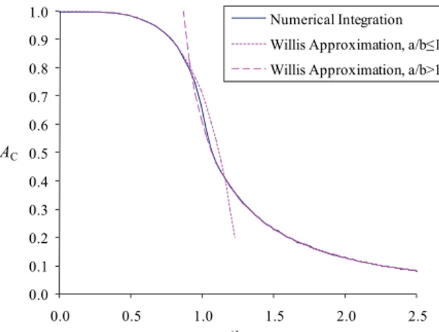
Both the numerical integration (10) and the approximation (14) for AC normalized with
respect to the area of a circle with radius b, πb2 as a function of ratio a/b is plotted in
Figure 4. The Willis equation (14) for the area seems to be a good approximation when compared to the actual area computed by the numerical integral.
Figure 4. Normalized area of a Cassini oval with numerical integration and Willis approximation 0.0 0.1 0.2 0.3 0.4 0.5 0.6 0.7 0.8 0.9 1.0 0.0 0.5 1.0 1.5 2.0 2.5 Numerical Integration Willis Approximation, a/b≤1 Willis Approximation, a/b>1
a/b AC
2.4. Perimeter of a Cassini Oval
To compute the perimeter, PC, of a Cassini oval, we follow a similar numerical
integration approach and depending on the symmetry property we multiply the arc length of a quarter oval by four. To do that, we use the infinitesimal calculus theorem which computes the arc length, S, of a function f(x) between x x l and
u
xx limits by a single integration.
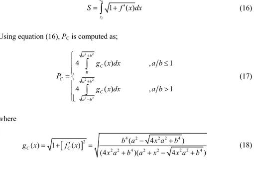
1 ( ) u l x x S
f x dx (16)Using equation (16), PC is computed as;
2 2 2 2 2 2 0 4 ( ) , 1 4 ( ) , 1 a b C C a b C a b g x dx a b P g x dx a b
(17) where
2 2 2 4 42 2 2 2 4 2 2 2 4 4 (4 )( ( ) ( 1 ( ) 4 ) ) C C b x a b x a b a x a g x f x a b x (18)As an alternative to numerical integration, we derive PC by hypergeometric
functions based on the parameters displayed in Figure 5 and computations in (Matz, 1985) as follows.
Figure 5. Cassini oval in Cartesian plane
In Figure 5 OP=r and 1
2
POD
. (Matz, 1985) uses using polar equations;
4 4 4 4 4 4 4 4 2 2 2 4 4 2 4 4 4 4 4 4 2 2 2 4 4 4 4 4 2 ( ) 4 [( ) ] cos 2 , sin 2 2 4 ( ) , [( ) ] 2 sin 2 4 [( ) ] b a r a r b a r a r a r d b a r rd b a r dr a r dr a r b a r (19)
and 2 2 2 4 4 4 4 1 1 2 2 ( ) 1 ( ) cos sin 2 2 2 a r b b a r ar a r (20)
Therefore when θ=0 it is true that 2 2 1
r b a and for θ=π/2, c
2 2
2
r b a . From that point by using the symmetry property, (Matz, 1985) c expresses PC as: 2 1 2 1 2 2 4 4 4 4 4 4 4 4 2 4 4 4 4 4 2 2 2 2 2 4 4 2 2 2 4 ( ) ( ) 4 4 ( ) 8 ( ) ( ) c C c c c a r b a r b a r P dr a r b a r r b dr b a r r b a
(21) restating, 4 ( 2 2 2) cos2 ( 2 2 2) sin2 r b a b a (22) follows, 2 2 2 1 2 2 2 2 2 2 2 2 4 2 sin cos ( ) cos ( ) sin b a r dr d b a b a (23)So equation (21) can be written by using (22) and (23) as follows (Matz, 1985): 1 2 2 1 2 2 2 2 2 2 2 2 2 2 4 0 1 2 2 1 2 2 2 2 4 0 4 ( ) ( ) ( ) sin 4 1 sin C d P b b a b a b a b d b a b
(24)At this point we can express PC by using hypergeometric functions as: 2 . ( , )
C
P b a b (25)
2 1 2 1 1, ,1, 4 2 ( , ) 4 1 a b a b (26) where2 1 1 1 , ,1, 4 2 is a Gauss-Hypergeometric function with parameters
1 4 , 1 2 , 1 and
2 2 1 a b a b .In the literature there are three approximations for PC all derived in (Matz, 1985).
Stating these approximations, in this study we display the best approximation that is derived by Taylor series in equation (27).
4 2 4 6 2 2 15 75 2 1 . 8 256 2048 C b P etc b a (27) where 2 2 2 2 2 2 4 ( ) b a b a .
The second approximation by (Matz, 1985) is:
4 2 2 2 2 2 2 2 2 2 2 2 2 2 2 2 2 2 2 2 2 2 4 2 2 2 2 2 2 2 2 2 2 ( ) ( )(2 ) ( ) ( ) 2 . ( ) 2 (2 ) ( ) ( ) ( )(2 ) .log ( ) C b b a b a a b b a b b a P b b a a b a b b a b b a b a a b b b a (28)
The third and final Matz approximation is by means of elliptic functions. The expression for the perimeter for a/b<1 (Matz, 1985) is:
2 2 2 2 2 2 1.3.5.7...(2 1) 2 1 . 1 1 2.4.6.8...2 n C n a a P b n b b
(29) for a/b=1,2 1.3.5.7...(2 1) 2 1 .2 2.4.6.8...2 n C n P a n
(30)and for a/b>1 the equation becomes:
2 2 2 2 2 2 2 1.3.5.7...(2 1) 2 1 1 1 2.4.6.8...2 n C b n b b P a a n a a
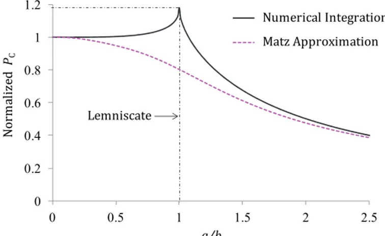
(31)Both the numerical integration (17) and the first Matz approximation (27) for PC
normalized with respect to the perimeter of a circle with radius b, 2πb as a function of ratio a/b is plotted in Figure 6. The actual normalized perimeter of a Cassini oval computed by numerical integration or hypergeometric functions gains a dent when a/b=1 and decreases as a/b ratio increases. The first Matz approximation seems to be a good approximation when a/b ratio is close to 0 and for a/b>2.
Figure 6. Normalized Perimeter of a Cassini oval
Also in (Willis, 2008) approximations for the area of a Cassini oval are given as in Table 1. If we call RR(max) and RR(min) as the maximum and minimum distances that
can be drawn from a foci to the border of an oval respectively; they are computed with the following formulae.
Table 1. Area and Max/Min Distances of a Cassini Oval
Case Distance Area (of one oval) RR(max) RR(min)
Circle 0 b2 b b One oval < 2b 2 (2 ) (64 )4 2 b a b (a2b2)12a (a2b2)12 a Two ovals > 2b b b2 2 (2 )a2 a(a2b2)12 (a2b2)12 a > 3b b b2 2 (2 )a2 b2 (2 )a b2 (2 )a 0 0.2 0.4 0.6 0.8 1 1.2 0 0.5 1 1.5 2 2.5 Numerical Integration Matz Approximation a/b Numerical Integration Matz Approximation No rm al iz ed PC Lemniscate
Figure 7. Normalized area and perimeter of a Cassini oval
Figure 7 is the plot of normalized values of both AC and PC with respect to the ratio
a/b. Note that the area gets its largest value when the oval is a regular circle (a/b=0) and gets a sudden decrease at around a/b=1 whereas the perimeter gets its largest value for a/b=1 and an increase in a/b accompanies a decrease both in the area and the perimeter. Therefore it can be inferred that in applications where the area or the perimeter of the oval is to be maximized, setting the a/b ratio at its relevant value as 0 and 1 respectively would be the optimal choice.
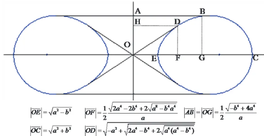
2.5. The Convex Hull and Interior Cover of a Cassini Oval
Let’s call Ce the convex hull of a Cassini oval and Ci the internal cover realized by a
closed elastic string drawn about the two foci F1 and F2 and crossing over at a point
O placed between them as in Figure 8. If e C
P and i C
P denote the perimeters of Ce
and Ci respectively, it is obvious that e C
P will be equal to PC fora b 2 2 and Ci
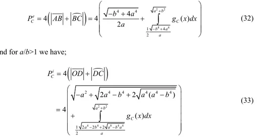
is 0 for a/b<1. Using information in Figure 8 we can compute e C P for a b 2 2 as follows:
2 2 4 4 4 4 1 4 2 4 4 4 ( ) 2 a b e C C b a a b a P AB BC g x dx a
(32)and for a/b>1 we have;
2 2 4 4 8 4 4 2 4 4 4 1 2 2 2 2 4 4 4 2 ( ) 4 ( ) 2 a b a i C a b C b a a P OD DC a b g x d a a a b x
(33)Figure 8. Intersection points of a Cassini oval on x-axis 2.6. Cassini Ovals as Sections of a Torus:
If we rotate the two-dimensional Cassini oval when 2 2a b1 around the vertical axis we get a three-dimensional shape of an oblate discsphere with a concavity on the top and bottom as seen in Figure 9.
Figure 9. Example of an oblate discsphere generated by rotating the Cassini oval on the left
By changing the parameters a and b we get different shapes having different diameter, thickness and concavity. However since those parameters are not directly related with the thickness or diameter the influence is an indirect one, therefore introducing a new parameter c we get a better flexibility for changing the three dimensional shape (Angelov, Mladenov, 2000).
Figure 10. Examples of oblate discspheres for various a, b and c parameters.
Let c be the radius of the generating circle. Let d be the distance from the center of the tube to directrix of the torus. The intersection of a plane p distant from the torus’ directrix is a Cassinian oval, with a=d and b2 4dp. One thing we realize is that for Cassini oval with large constant b2, the curve approaches a circle, and the
directix. That is a self intersecting torus without the hole which approaches to a sphere.
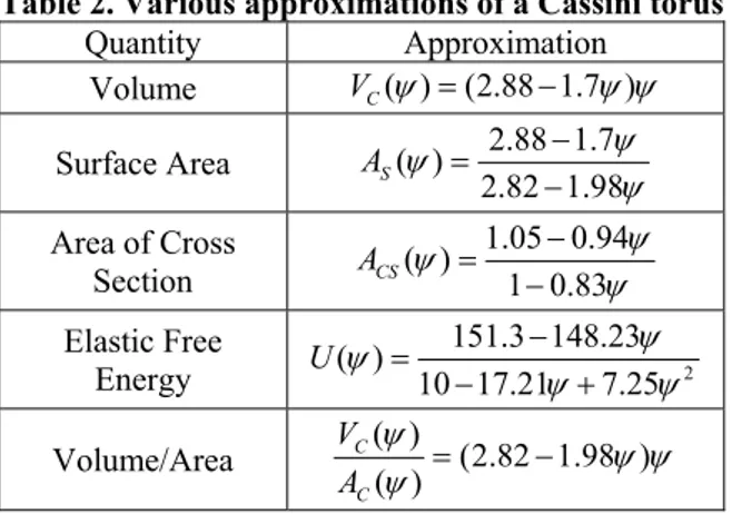
Table 2. Various approximations of a Cassini torus
Quantity Approximation Volume VC( ) (2.88 1.7 ) Surface Area ( ) 2.88 1.7 2.82 1.98 S A Area of Cross Section 1.05 0.94 ( ) 1 0.83 CS A Elastic Free Energy 2 151.3 148.23 ( ) 10 17.21 7.25 U Volume/Area ( ) (2.82 1.98 ) ( ) C C V A
In (Angelov, Mladenov, 2000) some useful measures of a Torus is approximated with an error of 1%. The approximated formulae in Table 2 is valid for the range
1 ,1 2
where a b. In Table 2 VC is the volume, AS is the surface area, ACS is the cross
section area and U is the elastic free energy of a torus (Angelov, Mladenov, 2000).
3. Applications
Cassinian curves are also utilized in various scientific applications such as nuclear physics, biosciences, acoustics, etc. Besides being a model for the orbit of planets, the multi foci closed curve, Cassini ovals, add new dimensions to analytical geometry (coordinate geometry) and other subjects related to mathematics beyond the prevailing concept of ellipse (Khilji, 2004). The unique geometrical properties that are discussed in the previous chapter are used for both military and commercial purposes. A few examples are; new generation bistatic radar and sonar systems, modeling human red blood cells, simulating light scattering, modeling textile fabric, modeling population growths, etc. that are discussed in detail below.
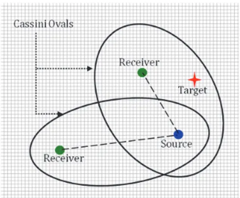
Military systems such as radars and sonars are the areas that the ovals are applied with a remarkable success. Radar and sonar systems are categorized as monostatic, bistatic and multistatic systems. A monostatic system is composed of a transmitter and a receiver located at the same place or in the same body. Radars originally made for monostatic use could be added a bistatic or multistatic mode by adding additional receivers spread out in the terrain as illustrated in Figure 11 or a set of netted radars could all operate in both mono and bistatic modes, adding increased complexity but also possibilities for better overall performance (Johnsen, Olsen, 2006). Similarly a multistatic sonar network consists of multiple sonar sources and receivers distributed over the surveillance area. Transmissions from one or more sources may be processed by one or more receivers to produce increased numbers of sonar echo contacts. Furthermore, this increased number of contacts comes from diverse source-receiver geometries and environmental conditions (Coraluppi,
Grimmett, 2003). Introducing the bistatic and multistatic concept, arises the problem of determining the effectiveness of such systems and utilizing the sensors for maximal coverage or probability of detection. Both in bi and multistatic radar and sonar systems the shape of the detection zone of the system is modeled with the interior of Cassini ovals (Cox, 1989) where the source, receiver and the target forms a bistatic triangle. Hence, to answer the questions mentioned here the geometrical properties such as the area, perimeter, convex hull, etc. are taken into consideration as in (Karataş, 2012) where the multistatic underwater sensor fields are optimized based on the shape and area of the ovals. Random fields of multistatic sensors are analyzed in (Washburn, 2010).
In nuclear science the theory suggests that the electron orbit will vary with the changes in the shape of the nucleus. It clubs the two great concepts; the concept of classical physics, an electron behaves as a particle and moves in standard orbits around the nucleus; and the concept of quantum mechanics which indicates the wave property of the electron and also the probability of the electron clouds (Beiser, 1997). Multi foci curve can be defined as a group curve in which the electron moves with a group velocity in the orbit. At that point the Cassini ovals are used to model the orbit of the electrons almost with no error (Beiser, 1997). In (Pashkevich, 1971) it is proved that the shape of the nucleus in the zeroth-order approximation is modeled with the Cassinian ovals, the deviation being expanded in a series of Legendre polynomials. As another example to nuclear science, in (Allen, Grove, Zanche, 2002) the cross-sectional area of a nuclear magnetic resonance coil that used to induce electrically conductive coil is modeled as a Cassini oval. Moreover, the coil induces a cylindrical body in the shape of a Cassini oval and a conducting shield with a cross sectional area substantially in the shape of another Cassini oval is formed around the cylindrical body.
Figure 11. Multistatic sensor network coverage defined by two Cassini ovals
An individual application in physics, Cassini ovals are a good fit for the simulation of light scattering by small particles. Although there are a great variety of methods to simulate the scattering which have been developed over the years the nullfield method with discrete sources is applied to analysis of light scattering by biconcave Cassini-like particles, which can be described as oblate discspheres with central concavities on their top and bottom (Angelov, Mladenov 2000). The appropriate mathematical description of the concave particle shapes that are used to simulate the light scattering is easily done by Cassini ovals. This kind of presentation is also used to approximate the shape of the human red blood cell as in (Angelov, Mladenov
2000; Mazeron, Muller, 1998; Di Biasio, Cametti, 2005) which is an exceptional application of the ovals in biology. Within such ovals the shape and volume changes in the red blood cells are modeled with negligible deviation and high confidence. Since Cassini ovals can be described as three parameters a, b and c, they can be easily implemented into computer algorithms, in Cartesian as well as polar coordinates to model the three-dimensional red blood cells and the properties pertinent to the ovals as sections of torus.
Cassinian ovals are also used to model evolutionary processes such as morphogenetic sequences (Koenderink, 1990) as well as to model the sub-atomic level and electro-magnetic activity in the case of wires of equal current and direction (Guangxi, Ximing, 1989).
In the report (Ryan, Verderaime, 1993) concerning the optimization of the fuel tanks used in Marshall Space Flight Center it is stated that "Tank end closures are usually elliptically shaped, but may not be the best configuration for performance and cost. The lox and fuel tank forward domes are designed primarily for internal pressure. Cassinian domes may provide as much volume as an ellipse in a shorter length and with less discontinuity at the edges for a total vehicle net weight saving." which is a good example of the miraculous shape of the ovals that is the best fit for fuel tanks. In (Daukantiene, Papreckiene, Gutauskas, 2003), the behavior of woven and knitted fabrics while pulling a disc-shaped specimen through a round hole of an experimental stand is analyzed by using some mathematical simulation models that are formed for this complicated process of textile deformation. At the end of the analysis of computational and experimental results it is shown that the best results are achieved by using models of the Cassini oval which have the sufficient precision and best reliability.
The ovals are also used as a model of population distribution between two regions where the spatial structures of population distribution are given. Such an example is in (Zong, Yang, Ma, Xue, 2009) where growth of population between the two metropolitan cities, Beijing and Tianjin of China which is a distinct dual-nuclei metropolitan area in the world, is modeled by the a/b characteristic index of Cassini ovals. In the study when a/b>1, the population density is more than 3000 persons/km2. When a/b=1, the population density is about 3000 persons/km2. For
√2/2<a/b<1, the density is between 500-3000 persons/km2 and so on. The results
show that owing to the combined action and influence of the regional dual-nuclei, the population distribution of Beijing-Tianjin region is in accord with Cassini model significantly.
A hash function is any algorithm or subroutine that maps large data sets of variable length, called keys, to smaller data sets of a fixed length (Hash function, 2012). In (Rusinol, Llados 2008) it is described how the hash function is formulated to be able to describe shapes in terms of the Cassinian ovals parameters, a and b, and how these parameters are used as indexing keys. The presented method aims to index large documents contained in large databases by the graphical symbols appearing in it by means of a hash table.
4. Summary and Conclusion
Although related to an ellipse for which the sum of the distances is constant, a Cassini oval has the product of the distances constant which makes it an interesting multi foci curve that is to be much better known than it is now. This unique property enables these ovals to be utilized in various scientific, military and commercial areas to model phonemes such as the detection zone of a bistatic radar/sonar, the orbit of the electrons, shape of the nucleus, the cross-sectional area of a nuclear magnetic resonance coil, light scattering by small particles, human red blood cell, the behavior of woven and knitted fabrics, population distribution between regions, mapping large data sets of variable length with hash functions, etc. Besides giving an overview and summary of the application areas of these magnificent ovals we also explore some of the useful properties of these curves, derive new analytical expressions for its area, perimeter, convex hull and interior cover in closed and open forms.
The parameters a and b where a is the semi-distance between the two foci and b is the constant which determines the exact shape of the curve is the starting point to understand how sensitive are the curves to the changes in those parameters, or the ratio a/b that is commonly used to identify the character of the curve, such as a single oval, a single oval with dents on the top and bottom or two disjoint mirror-imaged ovals. Another effect of the ratio is on the perimeter and area which get their maximum values for a/b =1 and a/b =0 respectively that can be computed with zero error by integrations in (10) and (17). The approximations in the literature are as in (14) and (27). The commonly used geometrical properties such as the length of the convex hull or interior cover can be numerically computed by equations (32) and (33) respectively. Moving from two-dimensions to three, the properties volume, surface area, area of cross section, elastic free energy of its torus can be approximated by the equations stated in Table 1.
This study is the first one in the literature that gives an overview of the properties of Cassini ovals as well as deriving new equations and creating a bridge between the unique properties and distinct applications in science, commerce, military, etc. Analyzing the analytical expressions in this paper, although there are no closed form analytical equations for the area and the perimeter of Cassini ovals in the literature, integrations stated in this paper can be effectively used to compute those properties without error. It is highly recommended to designers, planners or tactical decision makers to consider the sensitivity of the curve to the a/b ratio in terms of shape, area and perimeter, and to carefully adjust the distance between foci or the constant b to optimize their objectives.
5. Acknowledgments
The author would like to thank Prof. Alan R. Washburn in Naval Postgraduate School, Monterey, CA, USA for his guidance in this study.
This work was supported by the Scientific and Technological Research Council of Turkey (TUBITAK) (B.02.1.TBT.0.06.01-214-36-109)
6. References
ALLEN P.S., GROVE S., ZANCHE N. (2002). Nuclear magnetic resonance birdcage coil with Cassinian oval former. United States Patent, US 6,452,393 B1.
ANGELOV B., MLADENOV I.M. (2000). On the geometry of red blood cell. International Conference on Geometry, Integrability and Quantization, Coral Press, Sofia, pp.27-46. BEISER A. (1997). Concept of modern physics. Tata McGraw Hill Publishing Company Ltd.
N. Delhi. pp.131.
CORALUPPI S., GRIMMETT D. (2003). Multistatic sonar tracking. Signal Processing, Sensor Fusion, and Target Recognition XII, I KADAR (ed.), Proceedings of SPIE Vol. 5096.
COX, H. (1989). Fundamentals of bistatic active sonar. Underwater Acoustic Data Processing (Y. CHAN, ed.), Kluwer, pp.3-24.
DAUKANTIENE V., PAPRECKIENE L., GUTAUSKAS M. (2003). Simulation and application of the behaviour of a textile fabric while pulling it through a round hole. Fibres & Textiles in Eastern Europe, Vol 11-2, pp.41.
DI BIASIO A., CAMETTI C. (2005). Effect of the shape of human erythrocytes on the evaluation of the passive electrical properties of the cell membrane. Bioelectrochemistry. Vol 65-2, pp.163-169.
GIBSON K. (2007). The ovals of Cassini. Lecture Notes.
GILLESPIE C.C. (1971). Dictionary of scientific biography. New York: Charles Scribner’s Sons.
GLENN J.A., LITTLER G. H. (1984). A dictionary of mathematics. London: Harper and Row.
GUANGXI D., XIMING L. (1989). Approach to dynamics of fission described by Cassinian ovaloid. High Energy Physics and Nuclear Physics Journal, Vol 13-55, pp.8-455. Hash function. (2012). [Available at:] http://en.wikipedia.org/wiki/hash_function. [Accessed:
10.06.2012]
HELLMERS J., EREMINA E., WRIEDT T. (2006). Simulation of light scattering by biconcave Cassini ovals using the nullfield method with discrete sources. Journal of Optics A: Pure and Applied Optics, Pure Appl. Opt. Vol 8. pp. 1-9. HIRST A. E., LLOYD E. K. (1997). Cassini, his ovals, and a space probe to Saturn. The Mathematical Gazette, Vol 81, No. 492, pp.409-421.
JAMES G., JAMES R.C. (1949). Mathematics dictionary. D. Van Nostrand Co., Inc., New York. pp.39.
JOHNSEN T., OLSEN K.E. (2006). Bi and multistatic radar. Advanced Radar Signal and Data Processing, Vol. 4-1, pp.4-34.
KARATAŞ, M. (2012). Optimization of distributed underwater sensor networks with mixed integer non-linear programming. Marmara University Journal of Science, Vol. 24(3), pp.77-92.
KHILJI M.J (2004). Multi foci closed curves. Journal of Theoretics, Vol 6-6.
KOENDERINK J.J. (1990). Solid shape (Artificial intelligence). Massachusetts Institute of Technology, The MIT Press.
MATZ F. (1985). The Rectification of the Cassinian Oval by Means of Elliptic Functions, Am.Math. Monthly, Vol 2, pp.221-357.
MAZERON P., MULLER S. (1998). Dielectric or absorbing particles: EM surface fields and scattering. Journal of Optics, Vol 29, pp.68-77.
PASHKEVICH V.V. (1971). On the asymmetric deformation of fissioning nuclei. Nuclear Physics Journal, Vol 169-2, pp.275–293.
RAY K.S., RAY B.K. (2011). A method of deviation for drawing implicit curves. International Journal of Computer Graphics, Vol 2, No 2.
RUSINOL M., LLADOS J. (2008). A region-based hashing approach for symbol spotting in technical documents, graphics recognition. Recent Advances and New Opportunities, pp.104-113.
RYAN R., VERDERAIME V. (1993). Systems design analysis applied to launch vehicle configuration. NASA Technical Paper-3326.
SIVARDIERE J. (1994). Kepler ellipse or Cassini oval. European Journal of Physics, Vol 15, pp.62-84.
The New Encyclopedia Britannica (1987). Chicago, USA.
WASHBURN A. (2010). A multistatic sonobuoy theory. Technical Report, NPS-OR-10-005, Naval Postgraduate School, Monterey, CA.
WILLIS N.J. (2005). Bistatic radar. 2nd edition, SciTech Publishing.
WILLIS N.J. (2008). Bistatic radar. Radar Handbook. 3rd edition, M.I. SKOLNIK (Editor in
Chief), McGraw-Hill Professional, pp.23.4.
Wolfram Mathworld (2012). Cassini Ovals. [Available at:] http://mathworld. wolfram.com /CassiniOvals.html. [Accessed: 10.06.2012]
ZONG Y., YANG W., MA Q., XUE S. (2009). Cassini growth of population between two metropolitan cities - A case study of Beijing-Tianjin region. Chinese Geographical Science, Vol 19-3, pp.203-210.