A COMPARATIVE STUDY OF THE CAPABILITY OF ALTERNATIVE MIXED INTEGER PROGRAMMING FORMULATIONS

(1)

2018 Volume 24(2): 561–584 doi:10.3846/20294913.2016.1213202

Corresponding author Yusuf Tansel Ic E-mail: ytansel@baskent.edu.tr

A COMPARATIVE STUDY OF THE CAPABILITY OF ALTERNATIVE

MIXED INTEGER PROGRAMMING FORMULATIONS

Baris KECECI, Tusan DERYA, Esra DINLER, Yusuf Tansel IC Industrial EngineeringDepartment, Faculty of Engineering, Baskent University,

Eskisehir Yolu, 20. Km. 06810, Ankara, Turkey Received 30 June 2015; accepted 22 May 2016

Abstract. In selecting the best mixed integer linear programming (MILP) formulation the impor-tant issue is to figure out how to evaluate the performance of each candidate formulation in terms of selected criteria. The main objective of this study is to propose a systematic approach to guide the selection of the best MILP formulation among the alternatives according to the needs of the decision maker. For this reason we consider the problem of “selecting the most appropriate MILP formula-tion for a certain type of decision maker” as a multi-criteria decision making problem and present an integrated AHP-TOPSIS decision making methodology to select the most appropriate formula-tion. As an example the proposed decision making methodology is implemented on the selection of the MILP formulations of the Capacitated Vehicle Routing Problem (CVRP). A numerical example is provided for illustrative purposes. As a result, the proposed decision model can be a tool for the decision makers (here they are the scientists, engineers and practitioners) who intend to choose the appropriate mathematical model(s) among the alternatives according to their needs on their studies. The integrated AHP-TOPSIS approach can simply be incorporated into a computer-based decision support system since it has simplicity in both computation and application.

Keywords: capacitated vehicle routing problem, AHP, TOPSIS, multi-criteria analysis, optimiza-tion, operations research, mathematical model.

JEL Classification: C02, C44, C61, D81. Introduction

The modeling and optimization concepts are important for scientists, engineers and indus-trial practitioners. As computers are getting cheaper and more powerful and they are used more widespread, mathematical models play an increasingly important role in engineering optimization and it has become an increasingly cost-effective alternative to the experimen-tation. Besides, from an industrial point of view, the ability to understand and predict the real-world systems via mathematical modeling provides a distinct competitive advantage (Dobson 2003).

(2)

In most studies in the area of operations research (Luss, Rosenwein 1997; Pannirselvam

et al. 1999), the combinatorial optimization problems (COPs) are formulated as a mixed

integer linear programming (MILP) formulation and then they are solved by using either exact or meta-heuristic solution approaches. Also the solution of a COP can be obtained by solving the MILP formulation directly using an integer linear programming solver, as well.

Since everyone has a different knowledge-base and a unique way of looking at prob-lems, people may come up with different mathematical formulations for the same COP. In addition, different solution approaches for a problem may require the use of different formulations. Therefore, in the cases where there is more than one formulation (one can develop his/her own formulations in addition to already existing ones from the literature); we will try to answer the question of “which is the most appropriate formulation?” among the proposed candidates. It is important that selecting the best efficient formulation for a particular application depends on the needs of the solution approach and the nature of the problem to be optimized (Backlund et al. 2012).

In selecting the best MILP formulation, the important issue is to figure out how to evaluate the performance of each candidate formulation in terms of selected criteria. In most studies (see e.g, Gouveia, VoB 1995; Stadtler 1996; Sarin et al. 2005; Ordóñez et al. 2008; Öncan et al. 2009; Özgüven et al. 2010; Bektas et al. 2011; Ebadi, Moslehi 2012; Bek-tas 2012; Wu, Shi 2011; Wu et al. 2011, 2012) evaluation is based on some basic indicators, i.e. linear programming relaxation value (LPR), solution time, GAP value (this is defined as (U − L)/L, where U is the value of either the best or the optimal solution obtained within the time limit, and L is the value of the best lower bound after branching), and the number of optimally solved problems in a set of experiments. When dealing with small scale prob-lems which the optimal solution can be found in a reasonable time, the comparison of the mathematical formulations can be made easily by these basic indicators. However, when the problem size expands the optimal solution of the problem cannot be found in a reason-able time and it is difficult to find even a feasible solution. That’s why; the comparison of the formulations would not be so easy according to few basic indicators. Moreover taking into account just one or two criteria would lead to decide less efficient formulation. For example, when two different MILP formulations are compared within a given time, if we take into account only the value of the GAP value, the formulation which has the smaller GAP is chosen. However, the formulation which we choose with the smaller GAP may have a larger best integer objective value (upper bound) or may have a smaller best bound (lower bound). As well as in problems with minimizing objective function, the formulation with the largest LPR value is considered to be better. However when enough time is given, the formulation which has the worse LPR value may find the optimal solution in a shorter time. As Stadtler’s (1996) results also shows that “good bounds provided by an LPR do not guarantee that feasible solutions are found quickly”.

As mentioned above different approaches may require the use of different mathematical formulations. In the area of operations research (OR), a COP can be solved using either exact or meta-heuristic solution approaches. We refer these approaches as algorithms based on mathematical formulations. Those approaches use the proposed MILP formulation di-rectly or indidi-rectly in some part of the algorithm (Ball 2011). In this context assume that two different researcher types are defined; one tries to develop a heuristic or meta-heuristic

(3)

algorithm (an improvement type algorithm which starts from an initial feasible solution found by MILP formulation and tries to improve the solution quality) based on a MILP formulation and the other one tries to solve the COP by solving the MILP formulation di-rectly with solver software. According to this, on one side, the researcher who is interested in solving pure mathematical formulations, would prefer the formulation “which gives the optimal solution in shortest time”; on the other side, a researcher who is interested in model-based meta-heuristics would prefer the formulation “which gives the best quality feasible solution (that will be used as a starting feasible solution as good as possible in a fixed short time interval) in a shortest time”. For the reasons we try to explain above, se-lecting the most appropriate formulation for a particular use should be evaluated by taking into account other indicators as well.

The main objective of this study is to propose a systematic approach to guide the selec-tion of the best MILP formulaselec-tion among the set of alternatives according to the needs of the decision maker. The proposed systematic approach is not intended to be used in the comparison of alternative solution approaches (like heuristics or meta-heuristics), instead it is developed to be used in the comparison of alternative mathematical formulations those are desired to be used directly or indirectly in a specific solution approach. Thus, we consider the problem of “selecting the most appropriate MILP formulation for a certain type of decision maker” as a Multi-Criteria Decision Making (MCDM) problem and pres-ent an integrated Analytic Hierarchy Process, Technique for Order Preference by Similar-ity to Ideal Solution (AHP-TOPSIS) decision making model to select most appropriate formulation. The proposed decision model is implemented on the selection of the MILP formulations of the Capacitated Vehicle Routing Problem (CVRP). A numerical example is also provided for illustrative purposes. In the example, 7 different formulations which have been proposed within the CVRP literature were chosen and 8 criteria are determined. The AHP was used to prioritize the selected criteria. Each of the 27 test instances from the CVRP standard benchmark library were solved by each formulation and the performance values for each criterion were obtained. The criteria weights and the performance values of the mathematical formulations were combined by using the TOPSIS.

The remainder of this study is organized as follows: in Section 1, preliminary definitions on the MCDM methods are briefly given with their related literature. In Section 2, steps of the proposed model are shown. In Section 3, a numeric application for the proposed model is explained. Finally in the last section, conclusions and future research are discussed. 1. Definitions and preliminaries: MCDM

The selection of the most appropriate formulation can be regarded as an MCDM method where many criteria should be considered in the decision-making. There have been several MCDM methods developed in the literature (Vincke 1992; Zeleny 1982). Each method has its own characteristics and there are no better or worse techniques. However, some techniques better suit to particular decision problems than others do (Mergias et al. 2007; Dagdeviren et al. 2009). The most popular methods are scoring models (Nelson 1986), AHP (Ecer 2014; Ivlev et al. 2014; Myronidis et al. 2016; Singh, Nachtnebel 2016), Analytic

(4)

Network Process (ANP), Axiomatic Design (AD) (Khandekar et al. 2015), Utility Models (Munoz, Sheng 1995), TOPSIS (Liu 2009; Antuchevičiene et al. 2010; Maimoun et al. 2016), Elimination and Choice Translating Reality (ELECTRE) (Wang, Triantaphyllou 2008) and Preference Ranking Organization Method for Enrichment Evaluation (PROMETHEE) (Ka-bak, Dağdeviren 2014). These MCDM methods can be classified in many ways. One way is to classify them according to the type of data they use and another way is to classify them according to the number of decision makers involved in the decision process. According to the classification of Belton and Stewart (2002) there are value measurement models such as Multi-Attribute Utility Theory (MAUT) and AHP; goal aspiration and reference level mod-els such as TOPSIS; and at last outranking modmod-els such as ELECTRE and PROMETHEE.

It can be stated based on the authors’ literature survey that MCDM is the most com-mon approach applied for ranking alternatives. Acom-mong the MCDM approaches, the most used one is AHP because of its advantages over others (Wang, Chang 2007; Opasanon, Lertsanti 2013). As Saaty (1980) indicates, the most noted advantages of the AHP approach are; its ability to handle the inconsistencies in managerial judgments (perceptions); and its user friendly nature where users may directly input judgment data without any previous mathematical calculations. It can also be combined with other MCDM approaches and operations research models to allow users to structure complex problems in the form of a hierarchy or a set of integrated levels. The main objective and our motivation are to propose a systematic evaluation model to guide the selection of an effective formulation among a set of available alternatives by using the MCDM. Therefore, this study presents an MCDM model for the researchers which uses AHP to determine the importance weights of evalu-ation criteria, and TOPSIS to obtain the performance ratings of the feasible alternatives (Yurdakul, İç 2005; Dagdeviren et al. 2009; Tsai, Chang 2013; Kou et al. 2014; Hacioglu, Dincer 2015; Mandic et al. 2014; Prakash, Barua 2015). Although AHP and TOPSIS meth-ods are explained in the following sections, the readers are referred to Saaty (1980), Sen and Yang (1998), Yurdakul and İç (2005), Dagdeviren et al. (2009) for detailed explanations and application steps of AHP and TOPSIS methods. These approaches are implemented for three reasons: (a) it is easy and rational to apply; (b) the resulting table obtained from the solution of the formulations is directly used as the decision matrix of the TOPSIS; and (c) the importance weights obtained by AHP are included in the comparison procedures (Wang, Chang 2007).

2. The proposed model

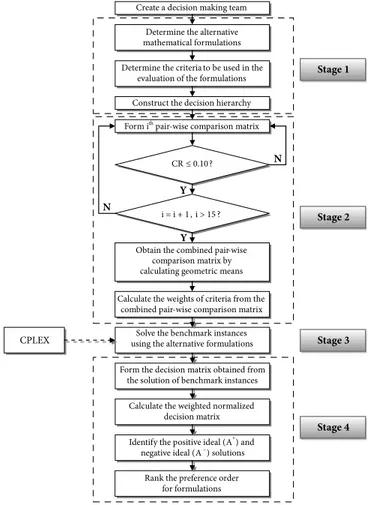
The proposed MCDM model for the evaluation of the mathematical formulations consists of the AHP and TOPSIS methods. This approach has four basic stages: (1) identifying the criteria to be used in the decision model and constructing the decision hierarchy, (2) calculating the weights of the criteria using the AHP computations, (3) solving each of the benchmark instances with each of the MILP formulations proposed for the understudy COP, (4) ranking the preference order of the alternative formulations with the TOPSIS. The flow diagram of the proposed decision model for the evaluation of the MILP formulations is provided in Figure 1.

(5)

Prior to the stages of the proposed decision model, a decision making team is created which consists of 15 researchers with OR background. According to Chang et al. (2008), expert opinions should be on a range from 10 to 30 and according to Robbins (1994) the decision making group probably should not be too large, i.e. a minimum of five to a maxi-mum of about 50. Therefore, for each type of decision maker, a decision team that consists of 15 researchers in the area of operations research is formed.

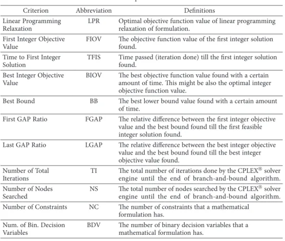
Possible criteria to be considered in the selection of the MILP formulations are deter-mined by the decision team with the use of the output that the CPLEX_{solver engine can} give. The criteria and their definitions and abbreviations are given in Table 1. The defini-tions of the criteria are given in the following:

Linear Programming Relaxation (LPR): It is the optimal objective function value of the

MILP formulation when the integrality restrictions of the variables are omitted. It gives the lower bound (for minimizing problem) and the bigger the LPR, the better the formulation is. Thus, it shows how tight (good) is the formulation.

Fig. 1. The flow diagram of the proposed decision model Create a decision making team

Determine the alternative mathematical formulations Determine the criteria to be used in the

evaluation of the formulations Construct the decision hierarchy

Stage 1

Form ith_{pair-wise comparison matrix} CR≤0.10?

Obtain the combined pair-wise comparison matrix by calculating geometric means

i = i + 1, i > 15? N Y N Y Stage 2

Calculate the weights of criteria from the combined pair-wise comparison matrix

Solve the benchmark instances using the alternative formulations Form the decision matrix obtained from

the solution of benchmark instances Calculate the weighted normalized

decision matrix

Stage 3

Identify the positive ideal (A*_{) and} negative ideal (A–_{) solutions}

Rank the preference order for formulations

Stage 4

(6)

Table 1. Criteria obtained from the CPLEX_{output and definitions}

Criterion Abbreviation Definitions

Linear Programming

Relaxation LPR Optimal objective function value of linear programming relaxation of formulation. First Integer Objective

Value FIOV The objective function value of the first integer solution found. Time to First Integer

Solution TFIS Time passed (iteration done) till the first integer solution found. Best Integer Objective

Value BIOV The best objective function value found with a certain amount of time. This might be also the optimal integer objective function value.

Best Bound BB The best lower bound value found with a certain amount of time.

First GAP Ratio FGAP The relative difference between the first integer objective value and the best bound found till the first feasible integer solution found.

Last GAP Ratio LGAP The relative difference between the best integer objective value and the best bound found till the best integer objective value found.

Number of Total

Iterations TI The total number of iterations done by the CPLEX _solver engine until the end of branch-and-bound algorithm. Number of Nodes

Searched NS The total number of nodes searched by the CPLEX _solver engine until the end of branch-and-bound algorithm. Number of Constraints NC The number of constraints that a mathematical

formulation has. Num. of Bin. Decision

Variables BDV The number of binary decision variables that a mathematical formulation has.

First Integer Objective Value (FIOV): It is the objective function value of the first feasible

solution found for the MILP formulation in the branch-and-bound tree. It gives the upper bound (for minimizing problem) and the lower the FIOV, the quicker the branch-and-bound may converge to the optimal solution.

Time to First Integer Solution (TFIS): It is an indicator of the time passed in seconds

until the first integer feasible solution is found during the CPLEX_{run. It shows how fast} a starting feasible integer solution (an upper bound for a minimizing problem) can be obtained. Especially for the researchers who use the MILP formulations for the model-based heuristics or the one who use the formulations for the exact solution algorithms, it may be beneficial to use the fastest formulation in terms of reaching first feasible integer solution, namely obtaining a starting feasible solution. So, the shorter the TFIS, the better the formulation is.

Best Integer Objective Value (BIOV): It is the objective function value of the best feasible

integer solution found within a given time limit. Other words it is the best upper bound (for minimizing problem) obtained. This value may be the optimal solution of the problem. Assume that there are two different formulations to be compared. When the optimal solu-tion is found by both formulasolu-tions within a given time limit for a specific test problem,

(7)

then this indicator does not make sense; since the BIOV of both formulations are the same. In this case, of course the solution time of the formulations is more decisive. However, when the size of a problem increases, then solving the problem optimally (or even to find a feasible integer solution) becomes more difficult. In such cases, the BIOV, if exists, may lead to decide which formulation is better. The lower the BIOV (for minimizing problem), the better the formulation is. In case the optimality is neglected (especially in practical applications where quicker decisions must be given in a limited time) the BIOV in a given time limit becomes more important than the optimal solution for both researchers and decision makers.

Best Bound (BB): It is the best lower bound (for minimizing problem) obtained in a

given time limit. Namely, it is the best objective function value of among the linearly re-laxed problems (nodes) solved in the branch-and-bound tree in a given time limit. Together with the upper bound value, the best bound shows how small the gap is. Withal, the larger “best bound” may lead the branch-and-bound algorithm converges to the optimal solution more quickly. So it can be said the bigger the BB, the better the formulation is.

First GAP Ratio (FGAP): It is the relative difference between the first integer objective

value and the best lower bound obtained till the first feasible integer solution found. It shows how small the starting feasible solution is relative to the current lower bound. So, it can be said the smaller the FGAP, the better the formulation is. However, this indicator may reveal another aspect of the formulations, different from the FIOV and BB since it gives a relative value. For example, when two different formulations are compared and if only the value of FGAP is considered, then the formulation with the smaller FGAP is chosen. However, the formulation which we choose with the smaller FGAP may have the bigger FIOV value or may have the smaller BB.

Last GAP Ratio (LGAP): It is the relative difference between the best integer objective

value and the best lower bound obtained till a given time limit is reached. Actually this value is calculated by using the BB and the BIOV. It shows how small the last (best) feasible solution (found so far) is relative to the BB. So it can be said smaller the LGAP, the better the formulation is.

Number of Total Iterations (TI): It is the total number of iterations done by the CPLEX solver engine till the end of the branch-and-bound algorithm. This indicator shows how fast the solver engine can solve a given MILP formulation in a predefined time limit. Thus it can be said, the bigger the TI, the better the formulation is. Instead of this value the ratio TI/Time may be considered as well.

Number of Nodes Searched (NS): It is the total number of nodes searched by the CPLEX solver engine till the end of the branch-and-bound algorithm. Like the TI, this indicator also shows how fast the solver engine can solve a given MILP formulation in a predefined time limit in terms of the nodes searched in the branch-and-bound tree. Thus it can be said, the bigger the NS, the better the formulation is. Instead of this value the ratio NS/ Time may be considered as well. There is a relation between the values TI and NS. That is, while solving a given MILP formulation, if the solver engine does more iteration per unit time, then it will search fewer nodes in the branch-and-bound tree or vice versa.

(8)

Number of Constraints (NC): It is the number of constraints that a MILP formulation

has. It shows how big the formulation is and it also effects directly the solution time of the relaxed formulations in each node in the branch-and-bound tree. Because when the number of constraints increases, the constant matrix (A) of the linear model increases and so to solve the simplex tableaus becomes harder. Hence it can be said the smaller the NC, the better the formulation is.

Number of Binary Decision Variables (BDV): It is the number of binary decision

vari-ables that a MILP formulation has. It shows how big the formulation is and also how big the branch-and-bound search tree is. When the number of binary variables increases, the number of nodes that must be searched in the branch-and-bound tree will increase expo-nentially. So it can be said the less the BDV, the better the MILP formulation is.

In the literature of the MCDM, Chen and Hwang (1992) advise a decision maker to gen-erate 7±2 criteria based on the Miller’s theory (Miller 1965). Also Saaty (1980) states that the criteria used for the application of AHP in a decision problem must be independent of each other (i.e. any criterion must not affect the others) and the number of the criteria should be around seven. This requirement is explained based on the fact that if the number of the criteria increases, the influence of each individual criterion decreases and this causes a decrease in sensitivity of the AHP. For this reason in this study, 8 of the 11 criteria are selected. FGAP and LGAP, are not considered since they are calculated by using FIOV, BIOV and BB (i.e. FGAP = FIOV/current best bound, LGAP = BIOV/BB). Also the criteria BDV is eliminated in advance since it does not mean anything because of the reason that the number of binary decision variables in the MILP formulations is same except the one presented in the Baldacci et al. (2004). One can choose a different set of criteria different from ours. For example the BDV criterion can be selected in the case where there is alterna-tive MILP formulations having different number of binary decision variables.

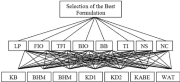
After the identification of criteria those are considered in the decision making problem, the decision hierarchy for the evaluation of MILP formulations is established. There are three levels in the decision hierarchy which are presented in Figure 2. The overall goal of the decision process determined as “the selection of the appropriate MILP formulation for a

certain type of decision maker” is in the first level of the hierarchy. The criteria are on the

second level and the alternative MILP formulations (abbreviations are given in Section 3) are on the third level of the hierarchy.

In the second stage, after the construction of the AHP hierarchy, the pair-wise compari-son matrices of the selected criteria are formed to determine the criteria weights. Each of the 15 researchers in the decision-making team makes their individual evaluations using the 1–9 scale proposed by Saaty (1980), to determine the values of the elements of pair-wise comparison matrices.

One of the important issues on the pair-wise comparison matrices is the consistency. Because in making pair-wise comparisons, errors arising out of inconsistency in judgments affect the final answer. The consistency of a decision matrix can simply be explained as follows: If a decision maker has judgments that ith_{criterion is α}

ij times important then jth_{criterion, and j}th_{criterion is β}

(9)

maker must judge the ith_{criterion is ∆}

ik = αijβjk times important then the kth criterion. Namely there must be transitivity on the judgments. Consistency Ratio (CR) is used to measure the inconsistency in the decision matrix. That’s why the CR value of each indi-vidual pair-wise comparison matrix is checked and in case of the inconsistency, the related matrix is revised by the same team participant until it will be consistent (Saaty 1980). On a scale from zero to one, the overall inconsistency should be below 10%.

Then all of the 15 pair-wise comparison matrices are reduced to one combined matrix whose elements are computed by calculating the geometric average of corresponding ele-ments in each of the matrices. This final matrix shows the joint point of view of the decision team on the importance of the criteria. Later on the weights of the criteria are calculated based on this combined comparison matrix.

In the third stage, the benchmark instances of the understudy COP are solved using the alternative MILP formulations. The decision matrix of the TOPSIS is formed by using this numerical values gathered within those solutions. In the fourth stage, the ranks of the MILP formulations are determined by using TOPSIS method. The formulation having the biggest

C_i*_{value (see Sen, Yang 1998; Yurdakul, İç 2005) is determined as the most appropriate} formulation according to the calculations by TOPSIS. Ranking of the other formulations is determined according to the C_i*_{values in descending order.}

3. The numerical application of the proposed model

In this section, as an application field, we choose the CVRP as the COP and the proposed decision model is implemented on the selection of the MILP formulations of the CVRP which have been presented in the literature.

The Vehicle Routing Problem (VRP) is one of the most studied combinatorial optimi-zation problem and is concerned with the optimal design of routes to be used by a fleet of vehicles to serve a set of customers. Since it was first proposed by Dantzig and Ramser (1959), for over 40 years the problem has been analyzed and tried to be solved using both exact optimization methods and heuristic algorithms (Baldacci et al. 2010).

The CVRP is the key operational problem that must be solved in the daily operation of physical distribution and logistics. Therefore the CVRP has been described as the most

(10)

common management problem in the food, fuel and the retail goods distribution. The CVRP applications has been studied by many researchers in the literature (Vaidyanathan

et al. 1999; Tan et al. 2001; Bell, McMullen 2004; Bektas 2006; Faulin, Juan 2008; Ji, Chen

2007; Eksioglu et al. 2009; Ali et al. 2009; Moghadam et al. 2010; Ezzatneshan 2010; Youse-fikhoshbakht, Sedighpour 2011; Soysal et al. 2015; Dominguez et al. 2016).

The CVRP can be defined as a problem of finding the m optimal routes from one cen-tral depot to a number of customers, in such a way that, each route starts and ends at the depot, each customer belongs to exactly one route, the load of a vehicle on each route does not exceed the capacity Q of the m identical vehicles, all customer demands are met by one vehicle and the sum of the total distance of all m routes is minimized. It is well known that the CVRP is an NP-hard (in the strong sense) problem (Haimovich et al. 1988; Ji, Chen 2007; Ali et al. 2009; Expósito-Izquierdo et al. 2016) and generalizes the well-known Traveling Salesman Problem (TSP).

A survey covering early exact methods for the CVRP is given by Laporte and Nobert (1987). The book edited by Toth and Vigo (2002) provides a comprehensive overview of CVRP and other variants proposed up to the end of the twentieth century (Baldacci et al. 2010). The most recent survey about the CVRP and exact solution algorithms is given by Cordeau et al. (2007) and Baldacci et al. (2010). The surveys of Laporte and Semet (2002) and of Gendreau et al. (2002) in the book edited by Toth and Vigo (2002) can be read for the researchers who are interested in the heuristic algorithms.

In this study, four different CVRP and three different Distance Constrained Capacitated Vehicle Routing Problem (DCVRP) formulations are considered. CVRP formulations are the formulation of Kara and Bektas (2005), two formulations of Baldacci et al. (2004) (one is multi-commodity flow formulation and the other is two-commodity flow formulation), and the formulation of Waters (1988). DCVRP formulations are the two formulations of Kara and Derya (2011) (one is node-based and the other is arc-based formulation), and the formulation of Kulkarni and Bhave (1985). Since we are interested in the formulations of the CVRP, we ignored the distance constraints and used only the capacity constraints in the DCVRP formulations. In this study, considered formulations are given with their abbreviations in the following: The Formulation of Kulkarni and Bhave (1985): KB; The Formulation of Baldacci, Hadjiconstantinou and Mingozzi (2004): BHM1; The Formulation of Baldacci, Hadjiconstantinou and Mingozzi (2004): BHM2; The Formulation of Waters (1988): WAT; The Formulation of Kara and Derya (2011) (Node Based Formulation): KD1; The Formulation of Kara and Derya (2011) (Arc Based Formulation); KD2; The Formula-tion of Kara and Bektaş (2005): KABE.

In the literature there are various mathematical formulations for the CVRP other than the ones considered above. Some of the formulations (see Toth, Vigo 2002: 12, 15, 21) even cannot be directly used to solve by a generic solver like CPLEX_{. The aim in this study is} not to compare all of the formulations in the CVRP literature, but to propose an MCDM method to select the appropriate formulation among the alternatives which can be solved directly by CPLEX_{. Hence, as a numerical application the most popular CVRP} formula-tions in the literature are chosen.

(11)

Suppose that there are three different types of researchers who are trying to solve the CVRP with different approaches using one of the proposed MILP formulations. So, those researchers will be the decision makers who intend to choose the appropriate mathemati-cal model(s) among the alternative candidates according to their needs on their ongoing studies. Assume that there is a decision maker who wants to find the optimal solution of the CVRP by just solving a MILP formulation (he/she would select) directly using a solver software. And we call this decision maker as “Decision Maker Type-1”. This type of decision makers would prefer the MILP formulation which finds the optimal solution in the shortest time. Also we define another decision maker who studies on an exact solution algorithm (i.e. a branch-and-cut or a branch-and-price algorithm which uses the MILP formulation he/she would select inside the algorithm) and wants to find the optimal solution of the CVRP by using the exact solution algorithm. We call this decision maker as “Decision Maker Type-2”. This type of decision makers would prefer the MILP formulation which gives the better lower and upper bounds.

Finally we assume a decision maker who studies on a heuristic or meta-heuristic algo-rithm (i.e. optimization based algoalgo-rithm which directly or indirectly uses the MILP for-mulation he/she would select inside the algorithm) and wants to find the optimal or near optimal solution of the CVRP by using the heuristic algorithm. We call this decision maker as “Decision Maker Type-3”. This type of decision makers would prefer the MILP formula-tion which gives the best starting feasible soluformula-tion in a shortest time. Each type of decision maker has its own preferences to choose the most appropriate MILP formulation.

The criteria to be used in the decision model are determined by the decision team with the use of the output that the CPLEX_{solver engine can give. Each member of decision} making teams makes individual judgments about the criteria to determine the values of the elements of pair-wise comparison matrices according to the preferences of the decision making team that reflects the type of decision maker. The numerical example is performed as it is provided on the steps in the Section 3 and the step by step explanations together with the results are given in the following sections.

3.1. Calculation of the weights of the criteria

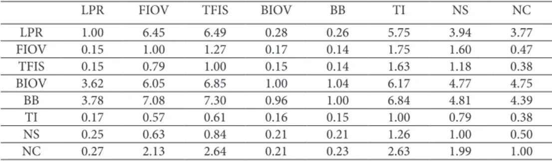
In the second stage of the proposed decision model, the weights of the selected criteria are calculated by using AHP method. In this stage, each member in each decision team makes individual judgments about the criteria by using the Saaty’s 1–9 scale (Saaty 1980) to determine the values of the elements of pair-wise comparison matrices according to the preferences of decision team that represents the corresponding Type of Decision Maker. Geometric averages of these values are found to obtain the combined pair-wise comparison matrix for each type of decision maker (Tables 2–4).

The weights of criteria obtained from the combined pair-wise matrices are given in Table 5 for each type of decision maker. CR value of the combined pair-wise comparison matrix is calculated for each type of decision maker and it is observed that they are all consistent since CR ≤ 0.1.

(12)

Table 2. The combined pair-wise comparison matrix for criteria according to decision maker Type-1

LPR FIOV TFIS BIOV BB TI NS NC

LPR 1.00 6.45 6.49 0.28 0.26 5.75 3.94 3.77 FIOV 0.15 1.00 1.27 0.17 0.14 1.75 1.60 0.47 TFIS 0.15 0.79 1.00 0.15 0.14 1.63 1.18 0.38 BIOV 3.62 6.05 6.85 1.00 1.04 6.17 4.77 4.75 BB 3.78 7.08 7.30 0.96 1.00 6.84 4.81 4.39 TI 0.17 0.57 0.61 0.16 0.15 1.00 0.79 0.38 NS 0.25 0.63 0.84 0.21 0.21 1.26 1.00 0.50 NC 0.27 2.13 2.64 0.21 0.23 2.63 1.99 1.00

Table 5. The weights of the criteria according to the decision maker Profile Weights

Criteria Decision Maker _Type-1 Decision Maker _Type-2 Decision Maker _Type-3

LPR 0.175 0.030 0.083 FIOV 0.043 0.067 0.300 TFIS 0.037 0.037 0.328 BIOV 0.297 0.225 0.050 BB 0.304 0.247 0.048 TI 0.031 0.086 0.090 NS 0.041 0.225 0.066 NC 0.072 0.083 0.034 CR 0.04 0.01 0.03

(13)

3.2. Establishing the decision matrix of the TOPSIS

After the weights of criteria are obtained for each type of the decision maker; at this stage before forming the decision matrix of TOPSIS method, the standard benchmark instances for the CVRP are solved by each of the seven MILP formulations. In these experimenta-tions twenty seven CVRP instances of Augerat et al. (1998) (Problem Set: A) which are available at http://www.branchandcut.org/ are used. The size of the test instances varies between 32 and 80 customers. The MILP formulations are coded in Optimization Program-ming Language (OPL) and solved using “CPLEX_{Optimization Studio Academic Research} Edition 12.2.0.2” on a PC with “Pentium Core 2 Quad 2.66 GHz processor and 2 GB of RAM” and running under “Ubuntu Server 10.10”. CPLEX_{parameters are set as follows;} node selection strategy: best-bound-search, search method: traditional branch-and-cut search, algorithm to solve sub-problems: primal simplex, variable selection strategy: strong branching, behavior when tree memory limit is reached: node file on disc and compressed, all other CPLEX_{parameters are left on default values. The time limit for the computation} time on CPLEX_{is set to 7200 seconds.}

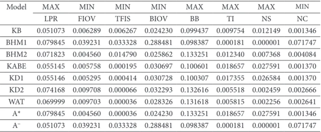
The average value of each criterion is obtained from the experimentations and given in Table 6. These values are used to construct the decision matrix of the TOPSIS method. In the application of the TOPSIS method, in the process of obtaining the ideal solutions, it is necessary to determine whether the criterion is in the cost or benefit class. This information is given in Table 6, as well. After obtaining the decision matrix, the normalized decision matrix is calculated and given in Table 7.

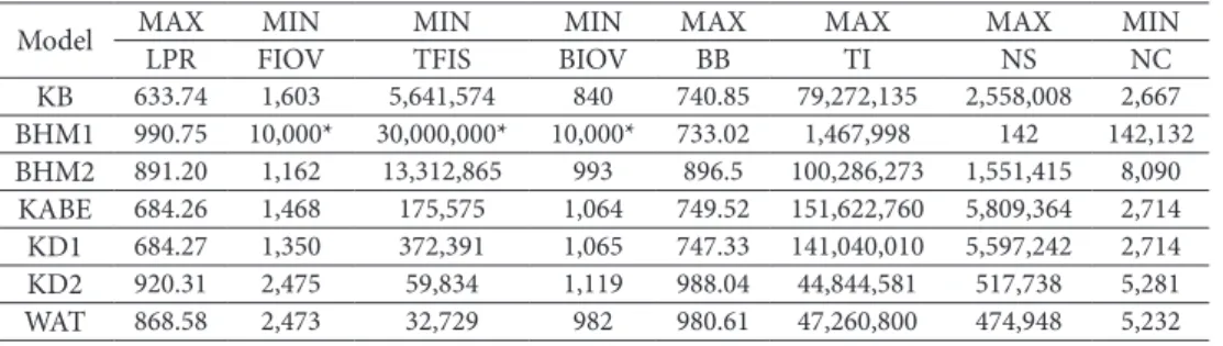
Table 6. Decision matrix obtained from CPLEX_solution

Model MAX_LPR _FIOVMIN MIN_TFIS _BIOVMIN MAX_BB MAX_TI MAX_NS MIN_NC KB 633.74 1,603 5,641,574 840 740.85 79,272,135 2,558,008 2,667 BHM1 990.75 10,000* 30,000,000* 10,000* 733.02 1,467,998 142 142,132 BHM2 891.20 1,162 13,312,865 993 896.5 100,286,273 1,551,415 8,090 KABE 684.26 1,468 175,575 1,064 749.52 151,622,760 5,809,364 2,714 KD1 684.27 1,350 372,391 1,065 747.33 141,040,010 5,597,242 2,714 KD2 920.31 2,475 59,834 1,119 988.04 44,844,581 517,738 5,281 WAT 868.58 2,473 32,729 982 980.61 47,260,800 474,948 5,232 Note: This value is chosen intentionally as very big (in the opposite direction of the benefit-cost in-formation of the criterion) since the formulation couldn’t give any value for none of the 27 instances during the given time limit.

Table 7. Normalized decision matrix

Model MAX_LPR _FIOVMIN MIN_TFIS _BIOVMIN MAX_BB MAX_TI MAX_NS MIN_NC

KB 0.29 0.15 0.17 0.08 0.33 0.31 0.30 0.02 BHM1 0.46 0.91 0.90 0.97 0.32 0.01 0.00 1.00 BHM2 0.41 0.11 0.40 0.09 0.44 0.40 0.18 0.06 KABE 0.32 0.13 0.01 0.10 0.33 0.60 0.67 0.02 KD1 0.32 0.12 0.01 0.10 0.33 0.56 0.65 0.02 KD2 0.42 0.23 0.00 0.11 0.44 0.18 0.06 0.04 WAT 0.40 0.23 0.00 0.10 0.43 0.19 0.06 0.04

(14)

3.3. Evaluation of the alternative formulations

After the solution of test instances are obtained and the decision matrix of the TOPSIS method is established; according to the three decision maker type the weighted normalized decision matrix is calculated by multiplying the normalized decision matrix by weights which are given in Table 5. Three weighted normalized decision matrices are obtained and the calculations are performed according to these matrices. After these calculations the positive ideal solution A*_{and negative ideal solution A}–_{are determined and these results} are presented in Tables 8–10.

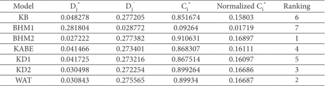
The distance of all alternatives to the positive ideal solution D_j*_{and the negative ideal} solution Dj– results are determined for all formulations and with these solutions the rela-tive closeness of each alternarela-tive to the ideal solution is obtained for each type of decision maker. According to these results, ranking of the alternatives are presented in Tables 11–13. Table 8. The weighted normalized decision matrix and the ideal solution values obtained by the deci-sion maker Type-1

Model MAX MIN MIN MIN MAX MAX MAX MIN

KB 0.051073 0.006289 0.006267 0.024230 0.099437 0.009754 0.012149 0.001346 BHM1 0.079845 0.039231 0.033328 0.288481 0.098387 0.000181 0.000001 0.071747 BHM2 0.071823 0.004560 0.014790 0.025862 0.133251 0.012340 0.007368 0.004084 KABE 0.055145 0.005758 0.000195 0.030697 0.100601 0.018657 0.027591 0.001370 KD1 0.055146 0.005295 0.000414 0.030728 0.100307 0.017355 0.026584 0.001370 KD2 0.074168 0.009708 0.000066 0.032293 0.132616 0.005518 0.002459 0.002666 WAT 0.069999 0.009703 0.000036 0.028326 0.131618 0.005815 0.002256 0.002641 A* 0.079845 0.004560 0.000036 0.024230 0.133251 0.018657 0.027591 0.001346 A– _{0.051073 0.039231 0.033328 0.288481 0.098387 0.000181 0.000001 0.071747}

Table 9. The weighted normalized decision matrix and the ideal solution values obtained by the deci-sion maker Type-2

KB 0.008755 0.009800 0.006267 0.018356 0.080793 0.027060 0.066672 0.001552 BHM1 0.013688 0.061127 0.033328 0.218546 0.079939 0.000501 0.000004 0.082709 BHM2 0.012312 0.007105 0.014790 0.019593 0.108267 0.034234 0.040436 0.004708 KABE 0.009453 0.008972 0.000195 0.023255 0.081738 0.051758 0.151415 0.001580 KD1 0.009454 0.008250 0.000414 0.023278 0.081499 0.048146 0.145886 0.001580 KD2 0.012715 0.015127 0.000066 0.024464 0.107751 0.015308 0.013494 0.003073 WAT 0.012000 0.015118 0.000036 0.021459 0.106940 0.016133 0.012379 0.003045 A* 0.013688 0.007105 0.000036 0.018356 0.108267 0.051758 0.151415 0.001552 A– _0.008755 _{0.061127 0.033328 0.218546 0.079939 0.000501 0.000004 0.082709}

(15)

Table 10. The weighted normalized decision matrix and the ideal solution values obtained by the deci-sion maker Type-3

KB 0.024223 0.043879 0.055560 0.004079 0.015701 0.028319 0.019557 0.000636 BHM1 0.037869 0.273704 0.295450 0.048566 0.015535 0.000524 0.000001 0.033881 BHM2 0.034064 0.031815 0.131109 0.004354 0.021040 0.035826 0.011861 0.001928 KABE 0.026154 0.040174 0.001729 0.005168 0.015884 0.054166 0.044415 0.000647 KD1 0.026155 0.036939 0.003667 0.005173 0.015838 0.050385 0.042793 0.000647 KD2 0.035177 0.067733 0.000589 0.005436 0.020939 0.016020 0.003958 0.001259 WAT 0.033200 0.067692 0.000322 0.004769 0.020782 0.016883 0.003631 0.001247 A* _{0.037869 0.031815 0.000322 0.004079 0.021040 0.054166 0.044415 0.000636} A¯ _{0.024223 0.273704 0.295450 0.048566 0.015535 0.000524 0.000001 0.033881}

Table 11. The ranking of formulations according to the decision maker Type-1

Model D_j* _D j¯ Ci* Normalized Ci* Ranking KB 0.048278 0.277205 0.851674 0.15803 6 BHM1 0.281804 0.028772 0.09264 0.01719 7 BHM2 0.027222 0.277382 0.910631 0.16897 1 KABE 0.041466 0.273401 0.868307 0.16111 4 KD1 0.041725 0.273216 0.867514 0.16097 5 KD2 0.030498 0.272254 0.899264 0.16686 3 WAT 0.030843 0.275565 0.89934 0.16687 2

(16)

3.4. The results of the numerical application

According to the results of AHP method in Table 5, the important criteria to compare the alternative formulations for the “Decision Maker Type-1” are BB, BIOV and LPR. Also the three most important criteria for the “Decision Maker Type-2” and “Decision Maker Type-3” are BB, BIOV, NS and TFIS, FIOV, TI, respectively.

Assume that the “Decision Maker Type-1” tried to decide according to only one cri-terion. In Table 5, the most important three criteria for the decision maker are BB, BIOV and LPR. The formulation of BHM1 would be chosen according to the LPR since it gives the best average value in Table 8 and the formulation of KB would be chosen according to the BIOV since it gives the best average value in Table 8. Thus, the decision maker might not decide which formulation is chosen. According to the results given in Table 11, the proposed approach gives the formulation of BHM2 in the first rank. In the case of handling crucial combination of criteria together according to the “Decision Maker Type-1”, the formulation of BHM2 will be selected by the proposed method.

The most important three criteria for the “Decision Maker Type-2” are the BIOV, BB and NS. If the decision maker considered only the BIOV (BB) then the formulation of KB (BHM2) would be chosen since it gives the best average value. Similarly the most impor-tant three criteria for the “Decision Maker Type-3” are the FIOV, TFIS and TI; and if the decision maker considered only the FIOV (TFIS) then the formulation of BHM2 (WAT) would be chosen since it gives the best average value. It would be pretty much confusing to decide which MILP formulation is the most appropriate one according to just one criterion. But with the application of decision model (by considering all predetermined criteria and their weights), however it can be seen that the formulation of KABE and KD1 have the first priority for the “Decision Maker Type-2” and “Decision Maker Type-3”, respectively. 3.5. Sensitivity analysis

To analyze and explore the response of AHP-TOPSIS decision model to the change in pri-orities of criteria, sensitivity analysis could be helpful. Sensitivity analysis is needed because for instance, sometimes the decision makers’ judgments may change if they have more information on the problem. According to the current judgments of the “Decision Maker Type-1”, the priority of “BHM2” is better than the other formulations. Also the “KABE” and “KD1” have the first priority according to the current judgments of the “Decision Maker Type-2” and “Type-3”, respectively. Hence, it is of importance to further analyze how the priority of formulations will change if the weights of criteria change. The changes in weights of chosen criteria are performed by Expert Choice 11 software. Expert Choice is a software package of the AHP. Decision makers can graphically change the weights of the criteria. In our decision model since the AHP is only used to calculate the weights of the criteria, the latter calculations of the sensitivity analysis are performed in Microsoft Excel to observe the changes of the ranking of different alternatives (here MILP formulations) systematically.

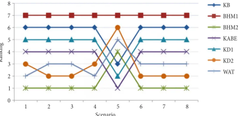
Eight scenarios are designed to do the sensitivity analysis of the decision problem. In each scenario only one of the criteria (LPR, FIOV, TFIS, BIOV, BB, TI, NS and NC) is increased by 25% from its current level. Figures 3–5 display how the (ranking of) alterna-tives perform with respect to the designed scenarios for each type of the decision maker.

(17)

Fig. 3. The result of designed scenarios for the decision maker Type-1

Fig. 4. The result of designed scenarios for the decision maker Type-2

Fig. 5. The result of designed scenarios for the decision maker Type-3 Scenario Rankin g 1 2 3 4 5 6 7 8 0 1 2 3 4 5 6 7 8 KB BHM1 BHM2 KABE KD1 KD2 WAT Scenario Rankin g 1 2 3 4 5 6 7 8 0 1 2 3 4 5 6 7 8 _KB BHM1 BHM2 KABE KD1 KD2 WAT Scenario Rankin g 1 2 3 4 5 6 7 8 0 1 2 3 4 5 6 7 8 KB BHM1 BHM2 KABE KD1 KD2 WAT

According to the judgments of “Decision Maker Type-1” (Fig. 3): In Scenario 5, in-creasing the weight of criterion BB by 25% decreases the ranking of formulation BHM2 from 1 to 4 (the global weight decreases from 0.16897 to 0.15961); besides the ranking of formulation KABE increases from 4 to 1 (the global weight increases from 0.16111 to 0.16595). In Scenario 5 it can be seen that the ranking of formulations affected

(18)

substan-tially by the change of the weight of BB. In Scenarios 2 and 3, it is also observed that the 25% increase in the weight of criteria FIOV and TFIS, respectively, change the ranking of formulations WAT and KD2. Figure 3 (scenario 5) indicates that increasing the weight of BB by 25% for the “Decision Maker Type-1”, will lead to the global weight of BHM2, WAT and KD2 showing a downward tendency and oppositely KABE, KD1 and KB showing an upward tendency. Figure 3 (scenarios 2 and 3) indicate that increasing the weight of FIOV and TFIS, respectively, by 25%, will lead to the global weight of KD2 showing an upward tendency and oppositely WAT showing a downward tendency.

According to the judgments of “Decision Maker Type-2” (Fig. 4): In Scenario 7, in-creasing the weight of criterion NS by 25% decreases the ranking of formulation KABE from 1 to 2 (the global weight decreases from 0.20511 to 0.19215); besides the ranking of formulation KD1 increases from 2 to 1 (the global weight increases from 0.20418 to 0.20672). There is not any change in the ranking of the formulations respect to the designed scenarios. Figure 4 (scenario 7) indicates that increasing the weight of NS by 25% for the “Decision Maker Type-2”, will lead to the global weight of KD1 showing an upward ten-dency and oppositely KABE showing a downward tenten-dency.

According to the judgments of “Decision Maker Type-3” (Fig. 5): In Scenario 3, increas-ing the weight of criterion TFIS by 25% decreases the rankincreas-ing of formulation KD1 from 1 to 2 (the global weight decreases from 0.18624 to 0.18261); besides the ranking of formu-lation KABE increases from 2 to 1 (the global weight increases from 0.18598 to 0.18723). In Scenario 2, it is also observed that the 25% increase in the weight of criterion FIOV, changes the ranking of formulations KB, WAT and KD2. Figure 5 (scenario 2) indicates that increasing the weight of FIOV by 25% for the “Decision Maker Type-3”, will lead to the global weight of KB showing an upward tendency and oppositely WAT and KD2 showing a downward tendency. Figure 5 (scenario 3) indicates that increasing the weight of TFIS by 25%, will lead to the global weight of KABE showing an upward tendency and oppositely KD1 showing a downward tendency.

The above situation demonstrates the conclusion of the sensitivity analysis. In general, KB has positive performance to increase in weights of BB and FIOV. BHM2 has negative performance to increase in weight of BB. KABE has positive performance to increase in weights of BB and TFIS, and has negative performance to increase in weight of NS. KD1 has positive performance to increase in weights of BB and NS, and has negative perfor-mance to increase in weight of TFIS. KD2 has negative perforperfor-mance to increase in weight of BB, and has positive performance to increase in weight of TFIS. WAT has negative per-formance to increase in weights of BB, FIOV and TFIS.

Conclusions and future researches

This study provides a systematic approach integrated with the AHP-TOPSIS methods to guide the selection of the most appropriate MILP formulation among the set of alternatives according to the needs of the decision maker. The proposed decision model is implemented on the selection of the MILP formulations of the CVRP in the literature. A numerical example is also provided for illustrative purposes. The usage of this model is especially

(19)

recommended when the MILP formulation is intended to be used in a solution approach of solving NP-hard COPs, since different approaches may require different requirements.

In the future studies, other COPs may be considered as a specific application field. The addition of other decision-maker type scenarios and the relationships among them can be added to the model for a more complete representation of the formulation’s performance, as well. In addition of this study, any other set of criteria may be used in the selection of MILP formulations. Also the dependencies between the criteria might be considered as a future research and the Analytic Network Process (ANP) can be used to determine the most appropriate formulations for the researchers in their own area of interest.

On the other hand future studies could extend the insights of this study in several options. For example, it would be interesting to develop a set of high-dimensional real case engineering optimization problems for comparing alternative MILP formulations. In this work, mathematical formulations are used, mainly because the number of dimen-sions could be scaled independently of the major features of the problem. However, real engineering optimization problems are likely to provide physical insights into the relative strengths and weaknesses of the methods that could prove useful to the practitioners.

The proposed decision model can be a tool for the decision makers (here they are the scientists, engineers and practitioners) who intend to choose the appropriate mathematical model(s) among the alternative candidates according to their needs on their ongoing stud-ies. The developed decision model is also easy to use, expandable, adaptable and modifi-able to different decision situations. The integrated AHP-TOPSIS approach can simply be incorporated into a computer-based decision support system since it has simplicity in both computation and application.

References

Ali, O.; Verlinden, B.; Oudheusden, D. V. 2009. Infield logistics planning for crop-harvesting operations, Engineering Optimization 41(2): 183–197. https://doi.org/10.1080/03052150802406540

Antuchevičiene, J.; Zavadskas, E. K.; Zakarevičius, A. 2010. Multiple criteria construction manage-ment decisions considering relations between criteria, Technological and Economic Developmanage-ment of Economy 16(1): 109–125. https://doi.org/10.3846/tede.2010.07

Augerat, P.; Belenguer, J. M.; Benavent, E.; Corberán, A.; Naddef, D.; Rinaldi, G. 1998. Computational re-sults with a branch and cut code for the capacitated vehicle routing problem. Research Report 949- M. Universite Joseph Fourier, Grenoble, France.

Backlund, P. B.; Shahan, D. W.; Seepersad, C. C. 2012. A comparative study of the scalability of alterna-tive meta-modelling techniques, Engineering Optimization 44(7): 767–786.

https://doi.org/10.1080/0305215X.2011.607817

Baldacci, R.; Hadjiconstantinou, E.; Mingozzi, A. 2004. An exact algorithm for the capacitated vehicle routing problem based on a two-commodity network flow formulation, Operations Research 52(5): 723–738. https://doi.org/10.1287/opre.1040.0111

Baldacci, R.; Toth, P.; Vigo, D. 2010. Exact algorithms for routing problems under vehicle capacity constraints, Annals of Operations Research 175(1): 213–245.

https://doi.org/10.1007/s10479-009-0650-0

Ball, M. O. 2011. Heuristics based on mathematical programming, Surveys in Operations Research and Management Science 16(1): 21–38. https://doi.org/10.1016/j.sorms.2010.07.001

(20)

Bektas, T. 2006.The multiple traveling salesman problem: an overview of formulations and solution procedures, Omega 34(3): 209–219. https://doi.org/10.1016/j.omega.2004.10.004

Bektas, T. 2012. Formulations and Benders decomposition algorithms for multidepot salesmen prob-lems with load balancing, European Journal of Operational Research 216(1): 83–93.

https://doi.org/10.1016/j.ejor.2011.07.020

Bektas, T.; Erdoğan, G.; Ropke, S. 2011. Formulations and branch-and-cut algorithms for the general-ized vehicle routing problem, Transportation Science 45(3): 299–316.

https://doi.org/10.1287/trsc.1100.0352

Bell, J. E.; McMullen, P. R. 2004. Ant colony optimization techniques for the vehicle routing problem, Advanced Engineering Informatics 18(1): 41–48. https://doi.org/10.1016/j.aei.2004.07.001

Belton, V.; Stewart, T. J. 2002. Multiple criteria decision analysis: an integrated approach. Boston: Kluwer Academic Publications. https://doi.org/10.1007/978-1-4615-1495-4

Chang, C. W.; Wu, C.-R.; Chen, H. C. 2008. Using expert technology to select unstable slicing machine to control wafer slicing quality via fuzzy AHP, Expert Systems with Applications 34(3): 2210–2220.

https://doi.org/10.1016/j.eswa.2007.02.042

Chen, S. J.; Hwang, C. L. 1992. Lecture notes in economics and mathematical systems. Berlin, Germany: Springer.

Cordeau, J. F.; Laporte, G.; Savelsbergh, M. W. P.; Vigo, D. 2007. Vehicle routing, Chapter 6 in C. Barn-hart, G. Laporte (Eds.). Handbooks in Operations Research and Management Science. Vol. 14. Am-sterdam: North-Holland, 367–428.

Dagdeviren, M.; Yavuz, S.; Kılınc, N. 2009. Weapon selection using the AHP and TOPSIS methods under fuzzy environment, Expert Systems with Applications 36(4): 8143–8151.

Dantzig, G. B.; Ramser, J. H. 1959. The truck dispatching problem, Management Science 6(1): 80–91.

https://doi.org/10.1287/mnsc.6.1.80

Dobson, D. C. 2003. Mathematical Modeling Lecture Notes [online], [cited 7 January 2003]. Available from Internet: http://www.math.utah.edu/~dobson/teach/540/notes.pdf

Dominguez, O.; Juan, A. A.; Barrios, B.; Faulin, J; Agustin, A. 2016. Using biased randomization for solving the two-dimensional loading vehicle routing problem with heterogeneous fleet, Annals of Operations Research 236(2): 383–404. https://doi.org/10.1007/s10479-014-1551-4

Ebadi, A.; Moslehi, G. 2012. Mathematical models for preemptive shop scheduling problems, Comput-ers and Operations Research 39(7): 1605–1614. https://doi.org/10.1016/j.cor.2011.09.013

Ecer, F. 2014. A hybrid banking websites quality evaluation model using AHP and COPRAS-G: a Tur-key case, Technological and Economic Development of Economy 20(4): 758–782.

https://doi.org/10.3846/20294913.2014.915596

Eksioglu, B.; Vural, A. V.; Reisman, A. 2009. The vehicle routing problem: a taxonomic review, Comput-ers and Industrial Engineering 57(4): 1472–1483. https://doi.org/10.1016/j.cie.2009.05.009

Expósito-Izquierdo, C.; Rossi, A.; Sevaux, M. 2016. A two-level solution approach to solve the clustered capacitated vehicle routing problem, Computers and Industrial Engineering 91: 274–289.

https://doi.org/10.1016/j.cie.2015.11.022

Ezzatneshan, A. 2010. A algorithm for the vehicle problem, International Journal of Advanced Robotic Systems 7(2): 125–132. https://doi.org/10.5772/9698

Faulin, J.; Juan, A. A. 2008. The ALGACEA-1 method for the capacitated vehicle routing problem, International Transactions in Operational Research 15(5): 599–621.

(21)

Gendreau, M.; Laporte, G.; Potvin, J.-Y. 2002. Metaheuristics for the Capacitated VRP, in P. Toth, D. Vigo (Eds.). SIAM monographs on discrete mathematics and applications. Philadelphia: SIAM, 129–154. https://doi.org/10.1137/1.9780898718515.ch6

Gouveia, L.; VoB, S. 1995. A classification of formulations for the (time-dependent) traveling salesman problem, European Journal of Operational Research 83(1): 69–82.

https://doi.org/10.1016/0377-2217(93)E0238-S

Hacioglu, U.; Dincer, H. 2015. A comparative performance evaluation on bipolar risks in emerging cap-ital markets using fuzzy AHP-TOPSIS and VIKOR approaches, Inzinerine Ekonomika-Engineering Economics 26(2): 118–129. https://doi.org/10.5755/j01.ee.26.2.3591

Haimovich, M.; Kan, A. H. G. R.; Stougie, L. 1988. Vehicle routing, methods and studies. Analysis of Heuristics for Vehicle Routing Problems, 47–61.

Ivlev, I.; Kneppo, P.; Bartak, M. 2014. Multicriteria decision analysis: a multifaceted approach to medi-cal equipment management, Technologimedi-cal and Economic Development of Economy 20(3): 576–589.

https://doi.org/10.3846/20294913.2014.943333

Ji, P.; Chen, K. 2007. The vehicle routing problem: the case of the Hong Kong postal service, Trans-portation Planning and Technology 30(2–3): 167–182. https://doi.org/10.1080/03081060701390841

Kabak, M.; Dağdeviren, M. 2014. A hybrid MCDM approach to assess the sustainability of students’ preferences for university selection, Technological and Economic Development of Economy 20(3): 391–418. https://doi.org/10.3846/20294913.2014.883340

Kara, I.; Bektas, T. 2005. Minimal load constrained vehicle routing problems, in V. S. Sunderam, G. D. van Albada, P. M. A. Sloot, J. J. Dongarra (Eds.). Computational Science – ICCS 2005. ICCS 2005. Lecture Notes in Computer Science. Vol 3514. Berlin Heidelberg: Springer-Verlag, 188–195.

https://doi.org/10.1007/11428831_24

Kara, I.; Derya, T. 2011. Polynomial size formulations for the distance and capacity constrained vehicle routing problem, in Numerical Analysis and Applied Mathematics ICNAAM 2011 AIP Conference Proceedings 1389, 19–25 September 2011, Halkidiki, Greece, 1713–1718.

Khandekar, A.; Antuchevičienė, V. J.; Chakraborty, S. 2015. Small hydro-power plant project selec-tion using fuzzy axiomatic design principles, Technological and Economic Development of Economy 21(5): 756–772. https://doi.org/10.3846/20294913.2015.1056282

Kou, G.; Peng, Y.; Lu, C. 2014. MCDM approach to evaluating bank loan default models, Technological and Economic Development of Economy 20(2): 292–311.

https://doi.org/10.3846/20294913.2014.913275

Kulkarni, R. V.; Bhave, P. R. 1985. Integer programming formulations of vehicle routing problems, Eu-ropean Journal of Operational Research 20(1): 58–67. https://doi.org/10.1016/0377-2217(85)90284-X

Laporte, G.; Nobert, Y. 1987. Exact algorithms for the vehicle routing problem, Annals of Discrete Mathematics 31: 147–184. https://doi.org/10.1016/s0304-0208(08)73235-3

Laporte, G.; Semet, F. 2002. Classical Heuristics for the Capacitated VRP, in P. Toth, D. Vigo (Eds.). SIAM monographs on discrete mathematics and applications. Vol. 9. The vehicle routing problem. Philadelphia: SIAM, 109–128.

Liu, P. 2009. Multi‐attribute decision‐making method research based on interval vague set and TOPSIS method, Technological and Economic Development of Economy 15(3): 453–463.

https://doi.org/10.3846/1392-8619.2009.15.453-463

Luss, H.; Rosenwein, M. B. 1997. Operations research applications: opportunities and accomplishments, European Journal of Operational Research 97(2): 220–244.

(22)

Maimoun, M.; Madani, K.; Reinhart, D. 2016. Multi-level multi-criteria analysis of alternative fuels for waste collection vehicles in the United States, Science of the Total Environment 550: 349–361.

https://doi.org/10.1016/j.scitotenv.2015.12.154

Mandic, K.; Delibasic, B.; Knezevic, S.; Benkovic, S. 2014. Analysis of the financial parameters of Ser-bian banks through the application of the fuzzy AHP and TOPSIS methods, Economic Modelling 43: 30–37. https://doi.org/10.1016/j.econmod.2014.07.036

Mergias, I.; Moustakas, K.; Papadopoulos, A.; Loizidou, M. 2007. Multi-criteria decision aid approach for the selection of the best compromise management scheme for ELVs: the case of Cyprus, Journal of Hazardous Materials 147(3): 706–717. https://doi.org/10.1016/j.jhazmat.2007.01.071

Miller, G. A. 1956. The magic number seven plus or minus two, Psychological Review 63(2): 81–97.

https://doi.org/10.1037/h0043158

Moghadam, B. F.; Sadjadi, S. J.; Seyedhosseini, S. M. 2010. Comparing mathematical and heuristic methods for robust vehicle routing problem, International Journal of Research and Reviews in Ap-plied Sciences 2(2): 108–116.

Munoz, A. A.; Sheng, P. 1995. An analytical approach for determining the environmental impact of machining processes, Journal of Materials Processing Technology 53(3–4): 736–758.

https://doi.org/10.1016/0924-0136(94)01764-R

Myronidis, D.; Papageorgiou, C.; Theophanous, S. 2016. Landslide susceptibility mapping based on landslide history and analytic hierarchy process (AHP), Nat Hazards 81(1): 245–263.

https://doi.org/10.1007/s11069-015-2075-1

Nelson, C. A. 1986. A scoring model for flexible manufacturing system project selection, European Journal of Operational Research 24(3): 346–359. https://doi.org/10.1016/0377-2217(86)90028-7

Öncan, T.; Altınel, I. K.; Laporte, G. 2009. A comparative analysis of several asymmetric traveling sales-man problem formulations, Computers and Operations Research 36(3): 637–654.

https://doi.org/10.1016/j.cor.2007.11.008

Opasanon, S.; Lertsanti, P. 2013. Impact analysis of logistics facility relocation using the analytic hier-archy process (AHP), International Transactions in Operational Research 20(3): 325–339.

https://doi.org/10.1111/itor.12002

Ordóñez, F.; Sungur, I.; Dessouky, M. 2008. A priori performance measures for arc-based formulations of vehicle routing problem, transportation research record, Journal of the Transportation Research Board 2032: 53–62. https://doi.org/10.3141/2032-07

Özgüven, C.; Özbakır, L.; Yavuz, Y. 2010. Mathematical models for job-shop scheduling problems with routing and process plan flexibility, Applied Mathematical Modelling 34(6): 1539–1548.

https://doi.org/10.1016/j.apm.2009.09.002

Pannirselvam, G. P.; Ferguson, L. A.; Ash, R. C.; Siferd, S. P. 1999. Operations management research: an update for the 1990s, Journal of Operations Management 18(1): 95–112.

https://doi.org/10.1016/S0272-6963(99)00009-1

Prakash, C.; Barua, M. K. 2015. Integration of AHP-TOPSIS method for prioritizing the solutions of reverse logistics adoption to overcome its barriers under fuzzy environment, Journal of Manufactur-ing Systems 37: 599–615. https://doi.org/10.1016/j.jmsy.2015.03.001

Robbins, S. P. 1994. Management. New Jersey, Prentice Hall.

Saaty, T. L. 1980. The Analytic Hierarchy Process. New York: McGraw-Hill.

Sarin, C. S.; Sherali, H. D.; Bhootra, A. 2005. New tighter polynomial length formulations for the asym-metric travelingsalesman problem with and without precedence constraints, Operations Research Letters 33(1): 62–70. https://doi.org/10.1016/j.orl.2004.03.007

(23)

Sen P.; Yang, J-B. 1998. Multiple criteria decision support in engineering design. London, Great Britain: Springer-Verlag London Limited. https://doi.org/10.1007/978-1-4471-3020-8

Singh, R. P.; Nachtnebel, H. P. 2016. Analytical hierarchy process (AHP) application for reinforcement of hydropower strategy in Nepal, Renewable and Sustainable Energy Reviews 55: 43–58.

https://doi.org/10.1016/j.rser.2015.10.138

Soysal M.; Bloemhof-Ruwaard, J. M.; Bektaş, T. 2015. The time-dependent two-echelon capacitated vehicle routing problem with environmental considerations, International Journal of Production Economics 164: 366–378. https://doi.org/10.1016/j.ijpe.2014.11.016

Stadtler, H. 1996. Mixed integer programming model formulations for dynamic multi-item multi-level capacitated lotsizing, European Journal of Operational Research 94(3): 561–581.

https://doi.org/10.1016/0377-2217(95)00094-1

Tan, K. C.; Lee, L. H.; Zhu, Q. L.; Ou, K. 2001. Heuristic methods for vehicle routing problem with time windows, Artificial Intelligence in Engineering 15(3): 281–295.

https://doi.org/10.1016/S0954-1810(01)00005-X

Toth, P.; Vigo, D. 2002. SIAM monographs on discrete mathematics and applications, Vol. 9, The Vehicle Routing Problem. Philadelphia: SIAM. https://doi.org/10.1137/1.9780898718515

Tsai, P.-H.; Chang, S.-C. 2013. Comparing the Apple iPad and non-Apple camp tablet PCs: a multicri-teria decision analysis, Technological and Economic Development of Economy 19(sup1): 256–284.

https://doi.org/10.3846/20294913.2013.881929

Vaidyanathan, B. S.; Matson, J. O.; Miller, D. M.; Matson, J. E. 1999. A capacitated vehicle routing problem for just-in- time, delivery, IIE Transactions 31(11): 1083–1092.

https://doi.org/10.1080/07408179908969909

Vincke, P. 1992. Multicriteria decision aid. New York: Wiley.

Wang, T. C.; Chang, T. H. 2007. Application of TOPSIS in evaluating initial training aircraft under a fuzzy environment, Expert Systems with Applications 33(4): 870–880.

Wang, X.; Triantaphyllou, E. 2008. Ranking irregularities when evaluating alternatives by using some ELECTRE methods, OMEGA 36(1): 45–63. https://doi.org/10.1016/j.omega.2005.12.003

Water, C. D. J. 1988. Expanding the scope of linear programming solutions for vehicle scheduling problems, International Journal of Management Science 16(6): 577–583.

https://doi.org/10.1016/0305-0483(88)90031-x

Wu, T.; Shi, L. 2011. Mathematical models for capacitated multi-level production planning problems with linked lot sizes, International Journal of Production Research 49(20): 6227–6247.

https://doi.org/10.1080/00207543.2010.535043

Wu, T.; Shi, L.; Geunes, J.; Akartunalı, K. 2011. An optimization framework for solving capacitated multi-level lot-sizing problems with backlogging, European Journal of Operational Research 214(2): 428–441. https://doi.org/10.1016/j.ejor.2011.04.029

Wu, T.; Shi, L.; Geunes, J.; Akartunalı, K. 2012. On the equivalence of strong formulations for ca-pacitated multi-level lot sizing problems with setup times, Journal of Global Optimization 53(4): 615–639. https://doi.org/10.1007/s10898-011-9728-8

Yousefikhoshbakht, M.; Sedighpour, M. 2011. An optimization algorithm for the capacitated vehicle routing problem based on ant colony system, Australian Journal of Basic and Applied Sciences 5(12): 2729–2737.

Yurdakul, M.; İç, Y. T. 2005. Development of a performance measurement model for manufacturing companies using the AHP and TOPSIS approaches, International Journal of Production Research 43(21): 4609–4641. https://doi.org/10.1080/00207540500161746

(24)

Baris KECECI. He is an Assistant Professor in the Department of Industrial Engineering at the Baskent

University. He received a PhD degree in Industrial Engineering from Gazi University Institute of Sci-ence and Technology. He has 3 years of experiSci-ence in private sector. His research interests include vehicle routing problems, mixed integer programming formulations, heuristic and exact algorithms, decision support systems, multi-criteria decision making.

Tusan DERYA. He is an Assistant Professor in the Department of Industrial Engineering at the Baskent

University. He received a PhD degree in Industrial Engineering from Gazi University Institute of Sci-ence and Technology. His research interests include assembly line balancing, vehicle routing problems, heuristic and exact algorithms, multi-criteria decision making.

Esra DINLER. She is an Instructor in the Department of Industrial Engineering at the Baskent

Uni-versity. She received a PhD degree in Industrial Engineering from Gazi University Institute of Science and Technology. She has 2 years of experience in private sector. Her research interests include produc-tion planning, recoverable systems, modeling and analysis of producproduc-tion systems, heuristic and exact algorithms, multi-criteria decision making.

Yusuf Tansel IC. He is an Associated Professor of Department of Industrial Engineering at the Baskent

University. He received a PhD degree in Mechanical Engineering from Gazi University Institute of Science and Technology. He has more than 10 years of experience in banking industry. His research interests include application of expert systems to manufacturing systems, modeling and analysis of production systems, decision support systems, multi-criteria decision making, and financial risk man-agement in commercial banks.